Curvature in the scaling relations of early-type galaxies

Abstract

We select a sample of about 50,000 early-type galaxies from the Sloan Digital Sky Survey (SDSS), calibrate fitting formulae which correct for known problems with photometric reductions of extended objects, apply these corrections, and then measure a number of pairwise scaling relations in the corrected sample. We show that, because they are not seeing corrected, the use of Petrosian-based quantities in magnitude limited surveys leads to biases, and suggest that this is one reason why Petrosian-based analyses of BCGs have failed to find significant differences from the bulk of the early-type population. These biases are not present when seeing-corrected parameters derived from deVaucouleur fits are used. Most of the scaling relations we study show evidence for curvature: the most luminous galaxies have smaller velocity dispersions, larger sizes, and fainter surface brightnesses than expected if there were no curvature. These statements remain true if we replace luminosities with stellar masses; they suggest that dissipation is less important at the massive end. There is curvature in the dynamical to stellar mass relation as well: the ratio of dynamical to stellar mass increases as stellar mass increases, but it curves upwards from this scaling both at small and large stellar masses. In all cases, the curvature at low masses becomes apparent when the sample becomes dominated by objects with stellar masses smaller than $3\times 10^{10}M_{\odot}$. We quantify all these trends using second order polynomials; these generally provide significantly better description of the data than linear fits, except at the least luminous end.

1 Introduction

Early-type galaxy observables, luminosities $L$, half-light radii $R_{e}$, mean surface brightnesses $I_{e}$, colors, and velocity dispersions $\sigma$, are strongly correlated with one another. These scaling relations are usually described as single power-laws ($R_{e}\propto L^{3/5}$, $\sigma\propto L^{1/4}$, $g-r\propto\sigma^{0.4}$, $R_{e}\propto I_{e}^{-0.8}$), suggesting a single formation mechanism across the population. However, galaxy formation models suggest that the brightest galaxies in clusters had unusual formation histories (De Lucia et al. 2006; Almeida et al. 2008), so they may follow different scaling laws (Boylan-Kolchin et al. 2005; Robertson et al. 2006; Hopkins et al. 2008a). Formation histories, and the importance of gaseous dissipation and/or gas rich mergers are also expected to have been different depending on the mass range of the galaxy (e.g. Mihos & Hernquist 1993; Naab et al. 2006; Hopkins et al. 2008b, Ciotti et al. 2007). So, one might reasonably expect to see departures from the single power-law scaling relations, especially at the extremes of the population.

Measurements of brightest cluster galaxy scaling relations have shown them to be unusual (Malumuth & Kirshner 1981, 1985; Oegerle & Hoessel 1991; Postman & Lauer 1995). And statistically significant detections of curvature in many scaling relations across the entire population have now been made (Zaritsky et al. 2006; Lauer et al. 2007; Bernardi et al. 2007; Desroches et al. 2007; Liu et al. 2008; but see von der Linden et al. 2007). The main goal of this paper is to exploit the large sample size provided by the Sloan Digital Sky Survey (hereafter SDSS) to make precision measurements of the curvature in these scaling relations.

Section 2 describes how we select a sample of early-type galaxies from the SDSS. It also discusses the corrections we apply to account for the fact that the SDSS photometric reductions are unreliable for extended objects. These are particularly important since the curvature we would like to measure is small (else it would have been seen in smaller samples), so the photometric and spectroscopic parameters at the extremes of the sample must be reliable.

Section 3 quantifies the curvature in a number of pairwise scaling relations for this sample. It also shows that, in the relations which involve luminosity, the curvature persists if one replaces luminosities with stellar masses. A final section summarizes our findings.

An Appendix discusses why, because they are not seeing-corrected, Petrosian based quantities are ill-suited for precision measurements in deep, magnitude-limited, ground-based datasets. It also shows why the Petrosian-based analysis of BCGs by von der Linden et al. (2007) yielded anomalous results.

2 The Sample

We start from a sample of 376471 galaxies based on the Fourth Data Release (DR4) of the SDSS but with parameters updated to the SDSS DR6 values (Adelman-McCarthy et al. 2008). From this sample we extract 46410 early-type galaxies following the procedure described below. We use SDSS deVaucouleur magnitudes and sizes, model colors, and aperture corrected velocity dispersions to $r_{e}/8$ unless stated otherwise. The SDSS also outputs Petrosian magnitudes and sizes. However, these are not seeing corrected, and Appendix A shows that this introduces systematic biases, so we do not use them in what follows. Throughout, angular diameter and luminosity distances were computed from the measured redshifts assuming a Hubble constant of $H_{0}=70$ km s^-1 Mpc^-1 in a geometrically flat background model dominated by a cosmological constant at the present time: $(\Omega_{0},\Lambda_{0})=(0.3,0.7)$.

About notation: we use $R_{e}$ to specify radius in kpc, and $r_{e}$ to specify angular size in arcseconds. For surface brightnesses, we use the following definition.

$$\mu_{e} = -2.5\log_{10}(I_{e})=-2.5\log_{10}\left(\frac{L}{2\pi R_{e}^{2}}\right)$$ (1)

$$= m+5\log_{10}(r_{e})+2.5\log_{10}(2\pi)-10\log_{10}(1+z)$$

where $m$ is the evolution, reddening, and k-corrected apparent magnitude. We use $M_{x}$ to denote the absolute magnitude in band $x$, and $M_{*}$ to denote stellar mass in solar units.

Figure 1: Comparison of the velocity dispersion measurements from the SDSS-DR6 and the IDLspec2d reduction. Vertical dashed line shows our cut at small $\sigma\sim 60$ km s^-1. Symbols with error bars show the median value and its uncertainty, dashed and dotted curves show the regions which enclose 68% and 95% of the objects.

2.1 Selecting early-types

To obtain a sample of early-type galaxies we first select the subset of galaxies which are very well-fit by a deVaucouleur profile in the $g$ and $r$ bands ($g$-band fracDev = 1 and $r$-band fracDev = 1); this gives about 100603 objects. To avoid contamination by later-type galaxies we also require the spectrum to be of “early-type”, by setting eClass $<0$ (see SDSS documentation for details of this classification). This slightly reduces the sample, to 94934 galaxies. Since the SDSS spectroscopic survey is magnitude limited, we require that $r-$band deVaucouleur magnitudes satisfy $14.5<m_{r}<17.5$. (Spectra are actually taken for objects having Petrosian magnitude $m_{r,Pet}<17.77$; our more conservative cut is designed to account for the fact that the Petrosian quantity systematically underestimates the total light in a deVaucouleur profile.) This cut leaves 70417 galaxies. Of these, 64492 have stellar mass estimates from Gallazzi et al. (2005).

We would also like to study the velocity dispersions of these objects. One of the important differences between the SDSS-DR6 and previous releases is that the low velocity dispersions ($\sigma<150$ km s^-1) were biased high; this has been corrected in the DR6 release (see DR6 documentation, or discussion in Bernardi 2007). We compared the values given by the official SDSS-DR6 database and those computed in the Princeton reduction (IDLspec2d). The two sets of measurements still show weak systematic trends. The upper panel of Figure 1 shows that at fixed $\sigma_{\rm DR6}$ the median values of $\sigma_{\rm IDLspec2d}$ agree quite well with the $\sigma_{\rm DR6}$ values, except at large $\sigma_{\rm DR6}>320$ km s^-1, where $\sigma_{\rm DR6}$ is slightly larger. However, the bottom panel shows that, when compared at fixed $\sigma_{\rm IDLspec2d}$, a systematic trend is more evident – especially at small $\sigma_{\rm IDLspec2d}<120$ km s^-1. To minimize systematics, we decided to average the DR6 and IDLspec2d velocity dispersion measurements.

Figure 2: Distribution of $b/a$ in the $r$-band as a function of angular (left) and physical size (right). Contours show regions of equal probability density. Starting at maximum density, each line represents a factor of $\sqrt{2}$ decrease in density. The change from solid to dotted lines marks the point which encloses 68% of the sample. There appears to be a separate population of small $b/a<0.6$ objects at physical sizes smaller than $a=10h^{-1}$ kpc.

At the low end, we select galaxies with $\sigma>60$ km s^-1 (see Section 3.4, Bernardi et al. 2003c and Hyde & Bernardi 2008 for discussion of biases introduced by eliminating objects based on their $\sigma$). At the high end we select galaxies with $\sigma<400$ km s^-1 to avoid contamination from double/multiple superpositions (see Bernardi et al. 2006b, 2008). The maximum $\sigma$ of a single galaxy given in Bernardi et al. 2008, and confirmed by Salviander et al. 2008 using high resolution spectra, is about 430 km s^-1. In addition, the SDSS-DR6 only reports velocity dispersions if the $S/N$ in the spectrum in the restframe $4000-5700$ Å is larger than 10 or with the status flag equal to 4 (i.e. this tends to exclude galaxies with emission lines). To avoid introducing a bias from these cuts, we have also estimated velocity dispersions for all the remaining objects. It turns out that this cut does not change the correlations studied here (nor those in the Fundamental Plane study of Hyde & Bernardi 2008). The net result is to change our sample from 64492 to 64343 objects. About 25 objects have colors which lie outside the range $0.4\leq g-r\leq 1.3$ which we do not believe, so we exclude them from the sample.

Figure 3: Histogram showing distribution of $b/a$ in the $g-$ (solid) and $r-$ (dashed) bands.

Figure 4: Dependence of axis-ratio $b/a$ on $a$ in the $r-$band for galaxies with $b/a>0.6$ in the $g-$band. Contours show the joint distribution of $b/a$ and $a$ with the same conventions for spacing and line styles as in Figure 2.

Figure 2 suggests that we should make one more cut. The left hand panel shows the distribution of axis ratios $b/a$ in the sample, as a function of the angular half light radius (left) and physical scale (right). There is clear evidence for two populations, particularly when plotted as a function of physical scale: one with $b/a>0.6$ and the other with $b/a<0.6$. The objects with small $b/a$ make up about twenty percent of our full early-type sample, but they are a larger fraction of the smaller fainter galaxies than they are of the bright. There are good physical reasons to suspect that these objects are a different population (e.g. rotational support is necessary if $b/a<0.6$), so, in what follows, we remove all objects with $b/a<0.6$ in the $g-$band from the sample. This leaves 51379 objects. Many of the figures which follow show quantities in the $r-$band, for which this cut appears less sharp. Figure 3 shows that the distribution of $b/a$ in the two bands is very similar: the small differences between $b/a$ in $g$ and $r$ is due, in part, to measurement error.

Figure 4 shows $b/a$ vs $a$ in the $r-$band in our sample after applying this cut. Comparison with Figure 2 shows that the ‘second’ population at low $b/a$ has been removed. In the sample which remains, there is a weak tendency for the largest galaxies to have slightly smaller $b/a$. The implications are discussed further in Bernardi et al. (2008) who show that the mean $b/a$ drops slightly at the highest luminosities and $\sigma$.

Finally, we must account for the fact that objects were brighter in the past by $0.9\,z$ mags because of stellar evolution (e.g. Bernardi et al. 2003a). This, with $k$-corrections, adjusts slightly the actual values of the magnitude limit which we should use when computing effective volumes. In fact, these effects work in opposite directions, so the net effect is small. However, since our goal is to quantify small effects in a large sample, it is necessary to do this carefully. The net result is to reduce the sample size by about ten percent, to 46410. As a check that this has been done correctly, we perform the test suggested by Schmidt (1968). If $V_{i}$ is the survey volume between object $i$ and the observer, and $V_{{\rm max},i}$ is the total survey volume over which the object could have been seen, then the average value of $(V/V_{\rm max})$ should be 0.5: we find $\langle V/V_{\rm max}\rangle=0.499$. (The luminosity evolution is slightly larger than, but statistically consistent with, the $0.85z$ mags reported by Bernardi et al. 2003b.)

These cuts are similar to those described by Bernardi et al. (2003a, 2006a), who provide further details about the motivation for each cut, except for: i) the cut on $b/a$; ii) the inclusion of velocity dispersions from low $S/N$ spectra or with the status flag not-equal to 4; and iii) the inclusion of velocity dispersions at $60<\sigma<90$ km s^-1. In addition, for the present study, we have chosen to be more conservative. Previously, we required Petrosian magnitudes $14.5<m_{r,{\rm Pet}}<17.75$. Changing to a brighter limit makes our final sample size considerably smaller than if we had used the Bernardi et al. (2006a) selection. In addition, we previously required fracDev $>0.8$ in the $r-$band; we now require fracDev $=1$ in $r$ as well as in $g$, because non-early-type features are expected to be more obvious in the $g-$ band. This more conservative choice for fracDev eliminated about 20000 objects (doing the selection based on $g$ but not $r$ makes little difference, because requiring fracDev $=1$ is quite stringent). To quantify the effect of these additional cuts, we have applied them to the Bernardi et al. (2006a) sample, and found that the comoving number density of objects is reduced to about 0.4 times that in Bernardi et al. (2006a). None of the results which follow are sensitive to the value of the comoving number density.

Figure 5: Comparison of GALMORPH and SDSS photometric reductions. Although the two are in good agreement at small $r_{e}$, where the bulk of the objects lie, the SDSS underestimates the total flux (top) and the half-light radius (middle) of large objects. However, both pipelines return consistent values of the quantity $\log_{10}(r_{e})-0.3\,\mu_{e}$ which Saglia et al. (2001) call FP. Symbols with error bars show the mean relation and its uncertainty, dashed and dotted curves show the regions which enclose 68% and 95% of the objects, and smooth solid curves show the fits given by equations (4) and (5).

Figure 6: Distribution of sizes obtained by the SDSS photometric reduction (solid) and corrected following Eq. 5 (dotted). Although the two are in good agreement at small $r_{e}$, where the bulk of the objects lie, the corrected sizes are larger for the small fraction of large $r_{e}$.

2.2 Corrections to photometry

We must address another issue before proceeding. This is because the SDSS reductions are known to suffer from sky subtraction problems, particularly for large objects (Adelman-McCarthy et al. 2008). To illustrate, Figure 5 compares SDSS photometric reductions with those of our own code, GALMORPH, for a subset of the full sample ($\sim 5500$ galaxies used by Bernardi et al. 2003a plus $\sim 180$ Bright Cluster Galaxies analyzed by Bernardi et al. 2007). The GALMORPH reductions do not suffer from the sky subtraction problem. This figure shows that while the two pipelines are in excellent agreement for small objects, the SDSS underestimates the sizes and brightnesses of large objects. However, the quantity IP $=\log{10}(r_{e})-0.3\,\mu_{e}$, identified by Saglia et al. (2001) (they called it FP), is not substantially changed. In all the panels, symbols with error bars show the mean relation and the error on the mean, dashed curves show the region encompassing 68% of the objects, and dotted curves enclose 95%.

Unfortunately, it is computationally expensive to run GALMORPH on the entire DR6 data release. Therefore, we have fit smooth curves to the trends shown in Figure 5 (solid curves) and we use these fits to correct the SDSS reductions as follows. Given $r_{\rm SDSS}$ we set

$$r_{e} = r_{\rm SDSS}+\Delta r_{\rm fit}(r_{\rm SDSS})$$ (2)

$$m = m_{\rm SDSS}+\Delta m_{\rm fit}(r_{\rm SDSS}),$$ (3)

where $r_{\rm SDSS}=r_{deV}\sqrt{\frac{b}{a}}$ is the SDSS-measured deVaucouleur radius expressed as a geometric mean ($\sqrt{ab}$) of the semimajor ($a$) and semiminor ($b$) axes of a half-light containing ellipse. $r_{deV}$, the semimajor axis length, and $\frac{b}{a}$, the axis ratio, are obtained from the SDSS catalogs where they are referred to as “deVRAD” and “devAB”, respectively. $\Delta r_{\rm fit}(r_{\rm SDSS})$ is zero if $r_{\rm SDSS}<2$ arcseconds and $\Delta m_{\rm fit}(r_{\rm SDSS})$ is zero if $r_{\rm SDSS}<1.5$ arcseconds, otherwise

$$\frac{\Delta m_{\rm fit}(r_{\rm SDSS})}{\rm mags} = 0.024279-\frac{r_{\rm SDSS}}{71.1734}-\left(\frac{r_{\rm SDSS}}{26.5}\right)^{2}$$ (4)

$$\frac{\Delta r_{\rm fit}(r_{\rm SDSS})}{\rm arcsec} = 0.181571-\frac{r_{\rm SDSS}}{4.5213}+\left(\frac{r_{\rm SDSS}}{3.9165}\right)^{2}$$ (5)

We propagate the errors similarly. Note that $-0.6\,\ln(10)\,r_{\rm SDSS}\,\Delta m_{\rm fit}$ provides a good approximation to $\Delta r_{\rm fit}$, as one might expect given the bottom panel in Figure 5; it slightly underestimates $\Delta r_{\rm fit}$ at large $r_{\rm SDSS}$. We have tested these corrections, and found them applicable to the SDSS $g$, $r$, and $i$ bands. Throughout the paper we will denote angular size in arcseconds with $r_{e}$ and physical size in ${\rm h^{-1}\ kpc}$ with $R_{e}$. These values refer to geometric-mean deVaucouleur radii, corrected as described in this section and Section 2.3.

Later in this paper, we will use stellar mass estimates from Gallazzi et al. (2005). These are derived by estimating a stellar mass-to-light ratio, and then multiplying by the estimated luminosity. Since our corrections to the apparent magnitudes will affect these luminosities (they increase slightly on average), we add equation (3) to Gallazzi et al. stellar mass estimates (accounting for the conversion from luminosity to magnitude, $m=-2.5\log_{10}L$). The net effect is to slightly increase some of the stellar masses, but we have not included a plot showing this increase.

Figure 6 shows the distribution of the effective radii of the 46410 early-type galaxies (i.e., whatever their $b/a$ value) before and after applying the correction given in equation (5). Although the two are in good agreement at small $r_{e}$, where the bulk of the objects lie, the corrected sizes are larger for the small fraction of objects with large $r_{e}$.

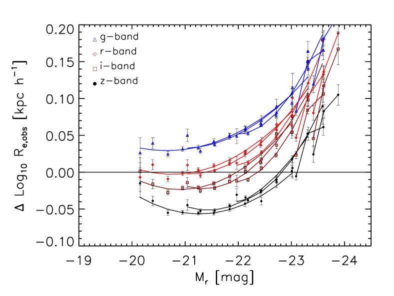
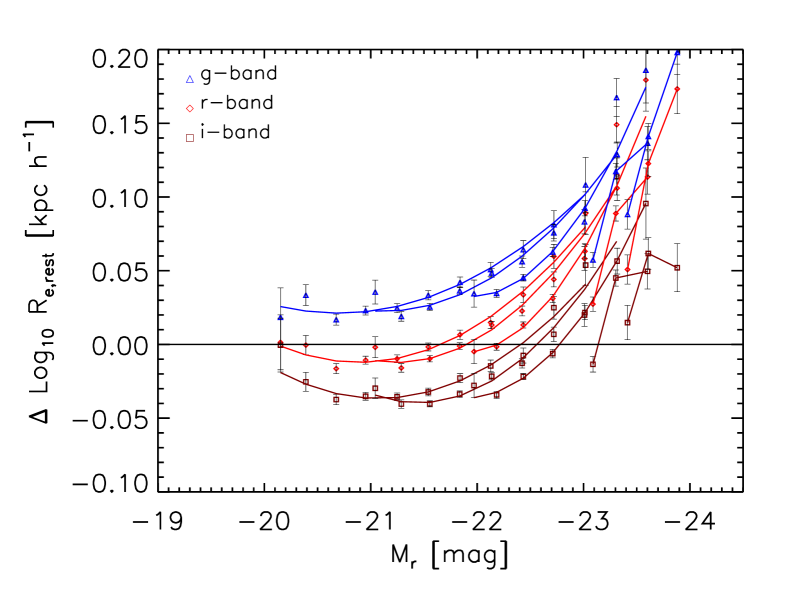
Figure 7: Observed (top) and corrected (bottom) sizes in the SDSS derived from deVaucouleur fits to the light profiles shown as a function of $r$-band luminosity $M_{r}$. (In all cases, $\Delta\log_{10}R_{e}\equiv\log_{10}R_{e}+0.22\,M_{r}+4.24$.) $g$-, $r$-, $i$-, and $z$-bands are shown from top to bottom in the upper panel. The bottom panel omits the $z$-band. In each panel, for each band, different lines show data from the following redshift bins: $0.07<z\leq 0.1$, $0.1<z\leq 0.13$, $0.15<z\leq 0.18$, $0.22<z\leq 0.25$ and $0.25<z\leq 0.35$.

2.3 Corrections to sizes

We make one final correction to the sizes, which is aimed at accounting for the fact that the early-type galaxies have color gradients: on average, their optical half-light radii are larger in bluer bands. If not accounted for, a population of intrinsically identical objects will appear to be slightly but systematically larger if they are at higher redshift. Our sample is large enough that we must correct for this effect, the moral equivalent of the $k$-correction to the luminosities. We do so following Bernardi et al. (2003a).

Table 1: Coefficients of best-fitting relations of the form $\langle Y|X\rangle=p_{0}+p_{1}\,X+p_{2}\,X^{2}$ to pairwise scaling relations. Fits were made to the binned points, not to the objects themselves. Linear fits ($p_{2}=0$) were made to the galaxies and restricted to the range $10.5<\log_{10}(M_{*}/M_{\odot})<11.5$ and $-23<M_{r}<-20.5$. The errors on the fitted coefficients are random errors: they depend on slope of the relation, its scatter, and the sample size. These are smaller than those produced by systematic effects (e.g., using $\sigma_{\rm DR6}$ or $\sigma_{\rm IDLspec2d}$ rather than their average). Typical systematics errors are a few times larger than the random errors.

Relation	$p_{0}\ \$	$p_{1}\ \$	$p_{2}\ \$	$\Delta\chi^{2}_{\nu}$
$\langle R|M_{*}\rangle$	$-4.79\pm 0.02$	$0.489\pm 0.002$	$-\ \$	$-\ \$
$\langle R|M_{*}\rangle$	$7.55\pm 0.44$	$-1.84\pm 0.08$	$0.110\pm 0.004$	$44.39$
$\langle V|M_{*}\rangle$	$-0.86\pm 0.02$	$0.286\pm 0.002$	$-\ \$	$-\ \$
$\langle V|M_{*}\rangle$	$-5.97\pm 0.27$	$1.24\pm 0.05$	$-0.044\pm 0.002$	$19.20$
$\langle I_{*}|M_{*}\rangle$	$-21.77\pm 0.09$	$-0.077\pm 0.009$	$-\ \$	$-\ \$
$\langle I_{*}|M_{*}\rangle$	$42.11\pm 2.23$	$-12.13\pm 0.41$	$0.57\pm 0.02$	$48.37$
$\langle R|M\rangle$	$-4.24\pm 0.02$	$-0.221\pm 0.001$	$-\ \$	$-\ \$
$\langle R|M\rangle$	$4.72\pm 0.32$	$0.63\pm 0.03$	$0.020\pm 0.001$	$38.70$
$\langle V|M\rangle$	$-0.32\pm 0.01$	$-0.119\pm 0.001$	$-\ \$	$-\ \$
$\langle V|M\rangle$	$-2.97\pm 0.23$	$-0.37\pm 0.02$	$-0.006\pm 0.001$	$6.21$
$\langle I|M\rangle$	$17.37\pm 0.08$	$-0.104\pm 0.004$	$-\ \$	$-\ \$
$\langle I|M\rangle$	$61.57\pm 1.61$	$4.10\pm 0.15$	$0.099\pm 0.003$	$37.96$
$\langle M_{dyn}/L_{r}|L_{r}\rangle$	$-1.50\pm 0.03$	$0.200\pm 0.003$	$-\ \$	$-\ \$
$\langle M_{dyn}/L_{r}|L_{r}\rangle$	$5.34\pm 0.70$	$-1.10\pm 0.13$	$0.062\pm 0.001$	$5.74$
$\langle M_{dyn}/M_{*}|M_{*}\rangle$	$-0.46\pm 0.02$	$0.062\pm 0.002$	$-\ \$	$-\ \$
$\langle M_{dyn}/M_{*}|M_{*}\rangle$	$2.25\pm 0.55$	$-0.48\pm 0.10$	$0.027\pm 0.005$	$1.44$
$\langle R|V\rangle$	$-1.42\pm 0.02$	$0.835\pm 0.008$	$-\ \$	$-\ \$
$\langle R|V\rangle$	$2.46\pm 0.23$	$-2.79\pm 0.20$	$0.84\pm 0.05$	$12.16$
$\langle I|R\rangle$	$-4.41\pm 0.03$	$0.246\pm 0.001$	$-\ \$	$-\ \$
$\langle I|R\rangle$	$-24.60\pm 0.57$	$2.30\pm 0.06$	$-0.052\pm 0.002$	$62.77$

We estimate the rest-frame radius in each band by interpolating the observed radii in adjacent bands. For example, to estimate the rest-frame $g$-band radius, we use the following expression:

$$R_{e,g,{\rm rest}}=\frac{(1+z)\lambda_{g}-\lambda_{r}}{\lambda_{g}-\lambda_{r}}\left(R_{e,g,{\rm obs}}-R_{e,r,{\rm obs}}\right)+R_{e,r,{\rm obs}}$$ (6)

where $\lambda_{g,r,i,z}=\{4686{\rm\AA},6165{\rm\AA},7481{\rm\AA},8931{\rm\AA}\}$ are the average wavelengths of the SDSS filters, and $z$ is the spectroscopically-determined redshift.

Figure 7 shows why this correction is necessary. It shows the sizes of objects in different bands as a function of $r$-band ($k$- and evolution-corrected) luminosity. To reduce the range of sizes, we have subtracted-off a luminosity dependent factor: we actually show $\Delta\log_{10}R_{e}\equiv\log_{10}(R_{e}/{\rm kpc})+0.221\,M_{r}+4.239$ (the reason for the exact choice of parameters will become clear shortly – see Table 1 – but note that, for the present purpose, the exact choice is not important). The upper panel shows the observed sizes: from top to bottom, the sets of symbols and lines show $g$-, $r$-, $i$-, and $z$-bands. For each band, different lines show data from a number of redshift bins: $0.07<z\leq 0.1$, $0.1<z\leq 0.13$, $0.15<z\leq 0.18$, $0.22<z\leq 0.25$ and $0.25<z\leq 0.35$. In any redshift bin, the sizes are clearly larger in $g$- and smaller in $i$- than they are in the $r$-band. The bottom panel shows rest-frame sizes, for $g$-, $r$-, and $i$-bands. We omit the $z$-band since longer wavelength observations would be necessary to reconstruct the $z$-band rest-frame size. The rest-frame sizes are indeed larger in the bluer bands, with the difference perhaps slightly smaller at large luminosity. The redshift dependence of the size-luminosity relation is not apparent when using the the observed radii (upper-panel), but can be seen when using the rest-frame radii (lower panel); this is studied further in Bernardi (2009).

The SDSS also outputs non-parametric Petrosian sizes. However, in contrast to the deVaucouleur-fitted quantities, these sizes are not corrected for the effects of seeing. The Appendix shows that, in contrast to the deVaucouleur sizes, the Petrosian sizes of objects at higher redshift are systematically larger than those from the model based fits. This is not surprising if seeing has compromised the Petrosian-based measurements, suggesting that, if this is not accounted for, then the use of Petrosian sizes limits or biases the precision measurements which large sample sizes would otherwise allow.

3 Curvature in scaling relations

We now turn to measurements of a number of scaling relations. It turns out that curvature is often even more obvious if we replace luminosity with stellar mass, so we will often show such relations side by side. Unless we specify otherwise, the luminosity is always from the $r$-band. We will sometimes use a shorthand for the $r$-band quantities: $R,V,I,M$ for $\log_{10}R_{e}$, $\log_{10}\sigma$, $\mu_{e}$, $M_{r}$.

3.1 Curvature in pairwise relations

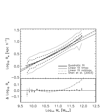
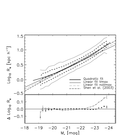
Figure 8: Half-light radius vs stellar mass and luminosity (left and right). Symbols with error bars show the median in small mass or luminosity bins, and dashed and dotted lines show the regions which contain 68% and 95% of the objects in each bin. Curves show fits of the form $\langle Y|X\rangle=p_{0}+p_{1}\,X+p_{2}\,X^{2}$ to these relations; best-fit coefficients are provided in Table 1. Curved fits were made to the binned counts (symbols with error bars), rather than to the objects themselves. Straight lines show linear fits to these relations; these were made to the galaxies and restricted to the range $10.5<\log_{10}(M_{*}/M_{\odot})<11.5$ and $-23<M_{r}<-20.5$. Bottom panels show residuals from the $V_{\rm max}^{-1}$-weighted linear (connected thin line) and quadratic fits (filled circles).

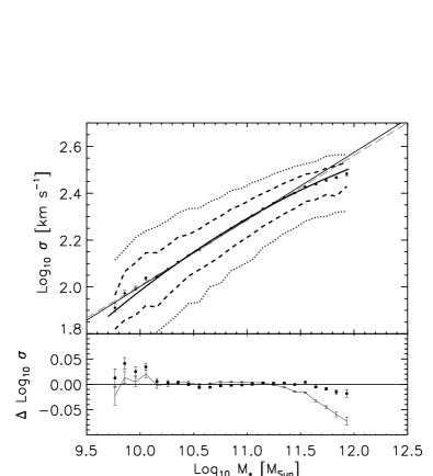
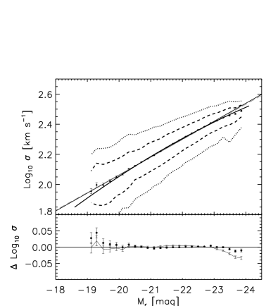
Figure 9: Same as previous figure, but for velocity dispersion.

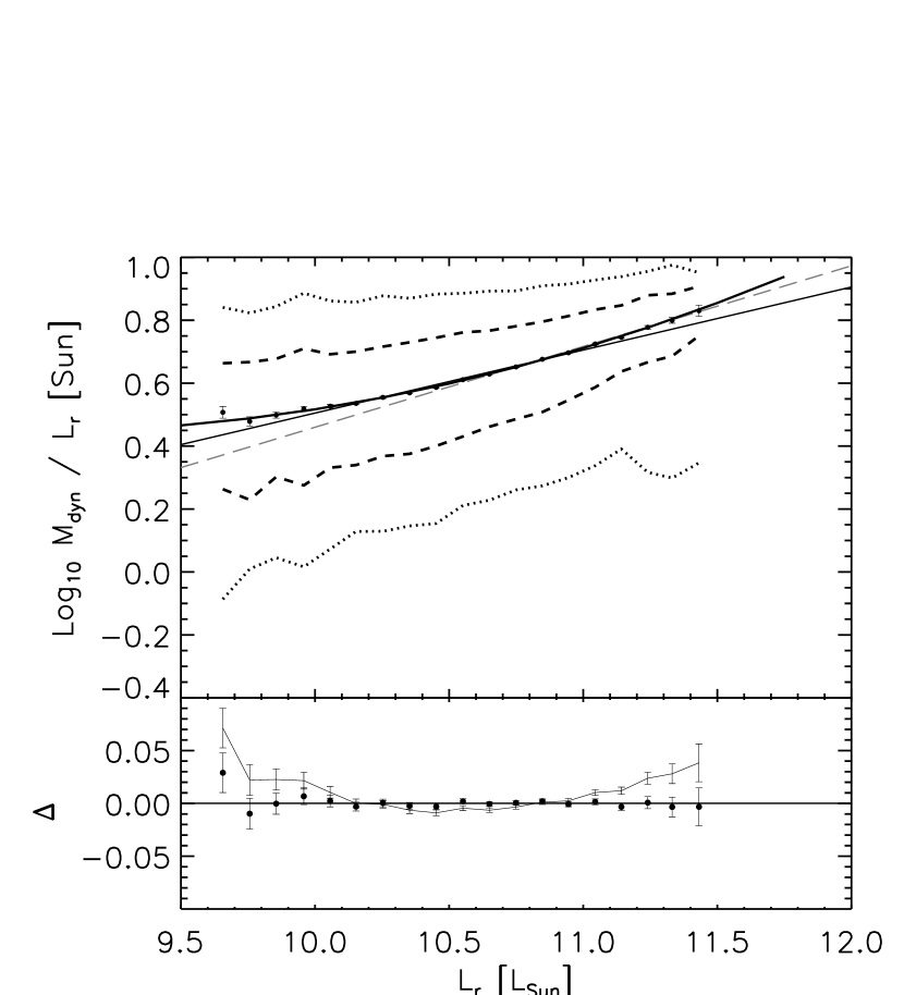
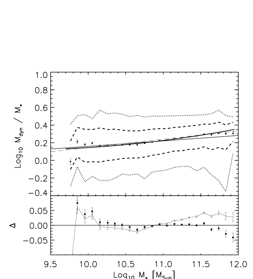
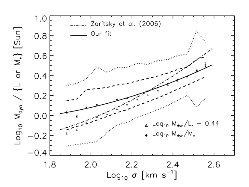
Figure 10: As for previous figure, but now for the ratio of dynamical mass to light versus luminosity (top) and dynamical to stellar mass versus $M_{*}$ (middle) and $M_{\rm dyn}/L$ or $M_{\rm dyn}/M_{*}$ versus $\sigma$ (bottom).

A simple test for curvature is as follows. In a magnitude limited survey, the more luminous objects are seen out to bigger volumes than the fainter objects, meaning that the ratio of the number of luminous to faint objects seen in such a survey is larger than the ratio of the true number densities of these objects. One can account for this over-abundance by weighting each object by $1/V_{\rm max}(L)$, the inverse of the volume over which it could have been seen; this down-weights luminous galaxies relative to fainter ones. If a scaling relation is a straight line, e.g., if the mean log(size) increases linearly as log(luminosity) increases, then the slope of the regression of $\log R$ on $\log L$ will not depend on whether or not one includes this weighting term. (This will also be true for $\log\sigma$ on $M$, etc.) However, if the intrinsic scaling relation is curved, then the slope of the regression line will depend on which weighting was used. This happens to be true in our dataset, indicating that the relations are curved: the slope of the $\log R-M$ relation is $-0.221\pm 0.001$ when weighting by $V_{\rm max}^{-1}$, but $-0.241$ when not. These numbers are $-0.119\pm 0.001$ and $-0.117$ for the $\log\sigma-M$ relation. The difference is more dramatic for the $\mu_{e}-M$ relation: $-0.104\pm 0.004$ and $-0.207$. Here, we reported the uncertainties due to random errors; uncertainties in the parameters due to systematics errors are a few times larger (see Section 3.2).

3.2 The size-luminosity relation

Recent work shows that the correlation between size and luminosity relation has evolved significantly since $z=2$ (e.g. Cimatti et al. 2008; van Dokkum et al. 2008). Bernardi (2009) shows that the sizes of luminous early-type galaxies ($M_{r}\sim-23$ mag) are still evolving at low redshift and that satellites are on average $\sim 8\%$ smaller than central galaxies. However, this last result is not seen for lower luminosity early-type galaxies (e.g. Weinmann et al. 2009). Due to this recent interest, we study this relation first, before considering others.

The symbols in the panels on the right of Figures 8 and 9 show the curvature in the size-luminosity and $\sigma$-luminosity relations, respectively (e.g. Lauer et al. 2007; Bernardi et al. 2007). This curvature is also evident when shown as a function of stellar mass (panels on the left), so curvature in the $M_{*}/L$ relation is not the only cause.

The format of this figure is similar to many that follow. The filled circles in the top panel show the median size in a number of narrow bins in luminosity, when the objects are weighted by $V_{\rm max}^{-1}$. Dashed and dotted curves show the regions which include 68% and 95% of the weighted counts. For statistics at fixed luminosity (as in this case), the $V_{\rm max}$ weighting makes no difference because, at fixed luminosity, all galaxies have the same weight. In Figure 12, which shows the $R-\sigma$ and $R-\mu_{e}$ relations, the difference is significant. There, we use open squares to show the median weighted count when no $V_{\rm max}$ weighting is used.

Straight solid and dashed lines show the result of fitting straight lines to the data, with and without $V_{\rm max}$ weighting. For distributions at fixed luminosity (as in this case), the two should be the same if the underlying scaling relation is not curved. If it is, then the fit to the unweighted points will reflect the slope of the relation at higher luminosities. In the case of the size-luminosity relation (Figure 8), the dashed line is steeper than the solid, consistent with the steepening of the relation at large $L$ shown by the symbols. In this case only, we also show the linear fits to the $R-L$ and $R-M_{*}$ relations reported by Shen et al. (2003) (see their Table 1, Fig. 6 and Table 1, Fig. 11 respectively). This shows that their fits are close to ours when we ignore the $V_{\rm max}$ weighting, but note that their sample is selected rather differently, and their sizes are from Sersic, rather than deVaucouleur fits to the light profile.

To quantify the curvature, we fit 2nd order polynomials to these and a number of other scaling relations (which follow). In all cases our fits are slightly non-standard because, to emphasize the curvature in these relations, we would like the fits to be sensitive to the tails of the distribution. Therefore, we have fit to the binned counts (i.e., the symbols) shown in the Figures, rather than to the objects themselves. For fits at fixed $L$, this is equivalent to weighting each object, not just by $V_{\rm max}^{-1}(L)$, but by $[V_{\rm max}(L)\phi(L)]^{-1}=[N_{\rm obs}(L)]^{-1}$. In effect, this upweights the tails of the distribution. The fitting minimizes $\chi^{2}$, defined as the sum of the squared distances to the binned points shown. If, instead, we weighted each of the binned points by (the inverse of its) error bar when defining $\chi^{2}$, then, because this additional weight is proportional to the number of counts in the bin, this would be the equivalent of weighting each object, rather than each binned point, equally.

The bottom panel shows residuals from the linear ($V_{\rm max}^{-1}$ weighted) and quadratic fits; in all cases, the residuals from the quadratic fits show fewer, if any, trends. Table 1 summarizes the results of these fits. Although the coefficients of the quadratic term appear to be very different from those when simply fitting a line, this is because we are reporting fits of the form $\langle Y|X\rangle=p_{0}+p_{1}\,X+p_{2}\,X^{2}$. Had we removed the mean values first, and fit $\langle y|x\rangle=p_{0}+p_{1}\,x+p_{2}\,[x^{2}-\langle x^{2}\rangle]$ instead (where $x=X-\langle X\rangle$, etc.) then $p_{1}$ would be very similar to linear fit, indicating that the curvature is small.

To quantify if a quadratic is a significantly better fit than a straight line, we fit both to the binned counts. We then compare $\chi^{2}_{\rm quad}/(N_{\rm bins}-3)$ with $\chi^{2}_{\rm line}/(N_{\rm bins}-2)$, where $\chi^{2}_{\rm quad}$ and $\chi^{2}_{\rm line}$ denote the minimized values of $\chi^{2}$, and the fits were to $N_{\rm bins}$ binned points. In all cases, this reduced value of $\chi^{2}$ for the quadratic is much closer to unity than for the linear fits. (Note that we do not use the coefficients of the linear fits to the unbinned counts that are shown in Table 1, since, for this test, we want to treat both the linear and quadratic fits equally. Of course, using these coefficients when computing $\chi^{2}_{\rm line}$ does not change our conclusions, since they can, at best, produce the same value of $\chi^{2}_{\rm line}$ which we have just described.)

Finally, a word on the errors on the fitted coefficients is in order. The numbers we quote are random errors: they depend on slope of the relation, its scatter, and the sample size. These are smaller than systematic effects: e.g., using $\sigma_{\rm DR6}$ or $\sigma_{\rm IDLspec2d}$ rather than their average makes a difference which is larger than the random error. Typical systematics errors are a few times larger than random errors – therefore, it is important to separate the two types of error.

Figure 8 shows that, compared to a single power law, the $R-L$ relation curves significantly towards larger sizes at large $L$ or $M_{*}$, consistent with previous work. At small $L$ or $M_{*}$ ($M_{r}<-19.5$ or $\log_{10}M_{*}/M_{\odot}<10.2$), the data appear to scatter slightly downwards from the quadratic fit. Although there are few objects in this tail, so the measurement is noisier, it is possible that this indicates that the sample is slightly contaminated at small $L$. We will return to this shortly.

Before we move on to other scaling relations, we note that results based on Petrosian quantities are shown in the Appendix, where we also discuss why we do not consider them further.

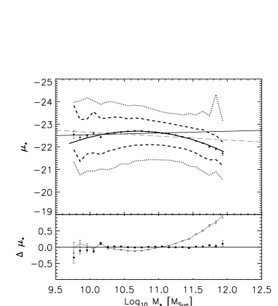
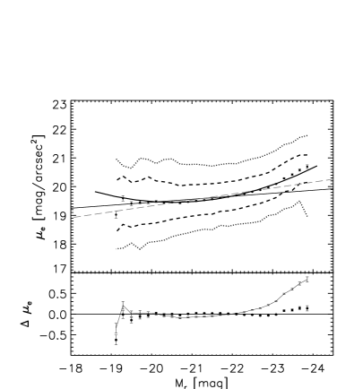
Figure 11: As for previous figure, but for stellar mass surface-brightness vs stellar mass (left) and surface-brightness vs luminosity (right).

3.3 Other scaling relations

Figure 9 shows the $\sigma-L$ relation in this sample. This relation is actually rather well described by a single power-law, except at $M_{r}<-23$ (where the mean value of $\log_{10}(\sigma/{\rm km~{}s^{-1}})>2.4$) where it curves slightly downwards. The flattening of the $\sigma-L$ relation is consistent with previous work, but notice that this effect is even more pronounced for the $\sigma-M_{*}$ relation.

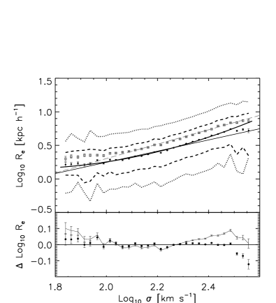
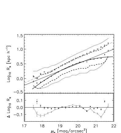
Figure 12: As for previous figure, but now for the size-velocity dispersion and size-surface-brightness relations.

Comparison with Figure 8 shows that, at large $M_{*}$ and $L$, the $R-L$ and $\sigma-L$ relations curve in opposite senses. Since dynamical mass $M_{\rm dyn}\propto R\sigma^{2}$, it is interesting to check if the $M_{\rm dyn}-L$ relation is well-fit by a simple power-law. We do this in Figure 10, where we set $M_{\rm dyn}\equiv 5\,R_{e}\sigma^{2}/G=4.65\times 10^{10}h^{-1}M_{\odot}\,(R_{e}/h^{-1}{\rm kpc})\,(\sigma/200~{}{\rm km~{}s}^{-1})^{2}$. The top panel shows that, at both small and large $L$, the $M_{\rm dyn}-L$ relation curves upwards from the $R\sigma^{2}\propto L^{0.2}$ scaling (solid line). The middle panel shows that curvature remains if one replaces $L$ with $M_{*}$, indicating that more than stellar population related effects are responsible. The slight rise at small masses is not implausible: star formation is expected to be less efficient at small masses. However, we view this with caution: the velocity dispersions at the small-mass end are more uncertain (e.g. Bernardi 2007). There is an average trend for $M_{\rm dyn}/M_{*}$ to increase with $M_{*}$, although it is weak: $\langle M_{dyn}/M_{*}|M_{dyn}\rangle\propto M_{*}^{0.062\pm 0.006}$ (the error 0.06 on the slope was computed accounting for systematics errors – the uncertainty from random errors is smaller $\sim 0.002$). The correlation between $M_{\rm dyn}/M_{*}$ with $M_{\rm dyn}$ is stronger: $\langle M_{dyn}/M_{*}|M_{dyn}\rangle\propto M_{dyn}^{0.17\pm 0.01}$ (see Figure 11 in Hyde & Bernardi 2008). If there were no scatter around this relation, then we would expect $\langle M_{dyn}/M_{*}|M_{*}\rangle\propto M_{*}^{0.17/0.83}\propto M_{*}^{0.2}$; because there is scatter, this scaling is shallower, $\propto M_{*}^{0.06\pm 0.01}$. Even if this relation were a simple power law without curvature, it would indicate that stars make up a smaller fraction of the total mass of a galaxy at large masses. This provides an important piece of information for adiabatic contraction based models of scaling laws (e.g. Padmanabhan et al. 2004; Lintott et al. 2005).

To connect with previous work, the bottom panel shows how $M_{\rm dyn}/L$ (triangles) and $M_{\rm dyn}/M_{*}$ (filled circles) scale with $\sigma$; both relations are slightly curved. Except at the largest $\sigma$, our data are relatively well described by the curved $M_{\rm dyn}/L-\sigma$ relation reported by Zaritsky et al. (2006) (we have shifted our measurements downwards by 0.44 dex because our data are in $r$ whereas their fit was in $I$, i.e. we use $r-I=1.1$. Note that we have also subtracted $-0.3$ from their fit since they used the effective light $L_{e}=L/2$, while we use the total light $L$). The fact that $M_{\rm dyn}/L$ is a steeper function of $\sigma$ than is $M_{\rm dyn}/M_{*}$ can be understood as follows. First, note that $M_{\rm dyn}/L=(M_{\rm dyn}/M_{*})\,(M_{*}/L)$. Then, note that $M_{*}/L$ increases with increasing $g-r$ color (e.g. Bell et al. 2004). However, $g-r$ color is strongly correlated with $\sigma$ – large $\sigma$ implies redder colors (Bernardi et al. 2005), and so $M_{*}/L$ increases with $\sigma$. Therefore, $M_{\rm dyn}/L$ increases with $\sigma$ because $M_{\rm dyn}/M_{*}$ does and because $M_{*}/L$ does so as well.

As a final study of curvature in relations which involve luminosity, we now turn to the $\mu_{e}-L$ and $\mu_{*}-M_{*}$ relations. (We define $\mu_{*}=-2.5\log_{10}(M_{*}/M_{\odot})+5\log_{10}(R_{e}/{\rm kpc})+2.5\log_{10}(2\pi)$; this is the stellar mass surface brightness within the half light radius.) Figure 11 shows that in this case too, there is significant curvature. However, the panel on the left shows that at $M_{*}<3\times 10^{10}M_{\odot}$, the $\mu_{*}-M_{*}$ relation becomes rather well fit by the linear relation, although it also becomes significantly noisier. A look back at the other relations which involve $M_{*}$ shows that they too become less well-defined at small $M_{*}$. This happens to be the same mass scale which Kauffmann et al. (2003) identify as being special.

It is possible that our early-type sample is contaminated by a different population at the low mass end – despite the fact that we have already tried to reduce such an effect by removing objects with $b/a<0.6$ and selecting galaxies with the $g$ and $r$-band fracDev $=1$. If we include those objects with $g$ and $r$-band fracDev $>0.8$ and/or do not remove objects with small $b/a$, then the quadratic remains a good fit even at small $M_{*}$ or $L$. This is also true if we simply use the cuts given by Kauffmann et al. (2003): ${\tt R90/R50}>2.86$, ${\tt R50}>1.6$ and $\mu_{50}<23$ mag$/$arcsec² in the $r$-band. We will return to this in the next subsection, but note that the curvature at the luminous, massive end of the sample, is highly significant.

We turn now to the scaling relations which play a fundamental role in the Fundamental Plane: the $R_{e}-\sigma$ and $R_{e}-\mu_{e}$ relations. Figure 12 shows that both these relations are curved. Notice that accounting for selection effects is important – the filled and empty symbols, which include or ignore the $V^{-1}_{\rm max}$ weight, trace very different relations. To first order, the zero-points of the two relations are more strongly affected than is the slope. Since it is the zero-point of the FP which is used to estimate evolution in small high-redshift samples, Figure 12 suggests that, without due care, one may simply be measuring selection effects (a point also made by Bernardi et al. 2003c).

Neither of these relations is as well-fit by a quadratic at the extremes; e.g., when weighted by $V^{-1}_{\rm max}$, the $R_{e}-\mu_{e}$ relation curves away significantly from the quadratic at both large and small $\mu_{e}$ (see also Nigoche-Netro et al. 2008). Curvature at large $\mu_{e}$ (or $\sigma$) is not surprising: we already know that BCGs, and more generally, large mass galaxies (Bernardi et al. 2008), follow different scaling relations. The flattening at small $\sigma$ is perhaps more surprising; this is in the regime where the SDSS velocity dispersions are most suspect, so one might worry that some of the effect is from measurement errors scattering objects to smaller $\sigma$. However, there is a similar flattening of the $R_{e}-\mu_{e}$ relation at $\mu_{e}<18$. What causes this?

3.4 Curvature from contamination?

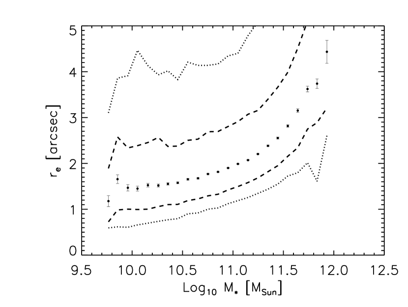
Figure 13: PCA eClass (top) and angular size (bottom) as a function of stellar mass. Later-type galaxies have less negative eClass values.

Figure 14: Similar to previous figures, but for the color-magnitude and color-stellar mass relations.

In the previous subsection we raised the possibility that the sample may be contaminated at low $M_{*}$. With this in mind, we performed a visual inspection of the objects with small $M_{*}$; this did not reveal any peculiarities. However, the top panel of Figure 13 shows the results of a PCA analysis of the spectra. A small departure from early- towards later-type values is seen at small-$M_{*}$, but note that true late-types have eClass values which are greater than zero. If we assume that some fraction $f$ of the sample has eClass = 0, and the rest has eClass = $-0.13$, then to find eClass = $-0.11$ requires $f\approx 0.15$. The true contamination is likely to be smaller (since eClass $>0$ for late-types).

Alternatively, one might have worried that this is an aperture effect associated with abundance gradients – the spectra are from fibers which take light from a fixed angular radius, so, for smaller galaxies, the light from the inner bulge contributes a decreasing fraction of the total light in the fiber. However, a plot of $r_{e}$ vs $M_{*}$ is approximately constant at small $M_{*}$ (bottom panel of Figure 13), suggesting that aperture effects are not to blame.

Finally, we note that the color-stellar mass and color-magnitude relations also show a small curvature, towards bluer colors, at small $L$ or $M_{*}$. The curvature in these relations is enhanced if we allow the full range of $b/a$ in our sample (rather than removing objects with $b/a<0.6$) and if objects with $g$ and $r$-band fracDev $>0.8$ are included (rather than selecting galaxies with fracDev $=1$). This, further circumstantial evidence for a small amount of contamination, is shown in Figure 14.

We have also studied what happens if we remove objects with $\sigma<90$ km s^-1. This is prompted by Figure 12, and also by the fact that Bernardi et al. (2003a) excluded such objects from their study of SDSS early-types (on the grounds that this is the regime in which the SDSS dispersions are suspect). Figure 15 shows that removing such objects has a dramatic effect on the scaling relations which involve surface brightness, since this preferentially removes objects with large sizes for their luminosities (or stellar masses). As a result, at the small mass end the size-luminosity (stellar mass) scaling relation leans towards smaller sizes. On the other hand, the $\sigma-L$ relation now flattens significantly at small $L$, because the small $\sigma$s at small $L$ have been removed (there are essentially no objects with small $\sigma$ at large $L$), and the luminosity-$\mu_{e}$ flattens significantly. In addition, $M_{\rm dyn}/M_{*}$ vs $M_{*}$ becomes more curved because, for a given $M_{*}$, one is removing small $M_{\rm dyn}$. This leaves only large values of $M_{\rm dyn}/M_{*}$ at small $M_{*}$, making the relation curve upwards steeply. See Hyde & Bernardi (2008) for further discussion of the dramatic effects that cuts in $\sigma$ can have on the Fundamental Plane (also see Bernardi et al. 2003c).

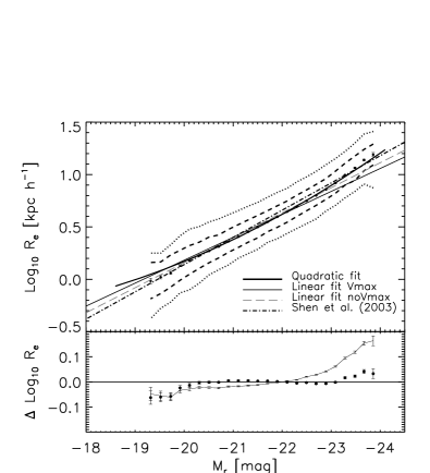
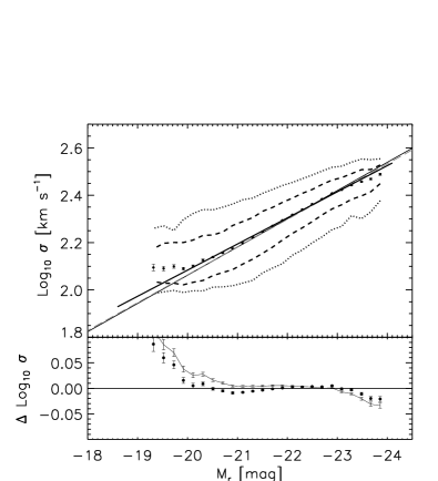
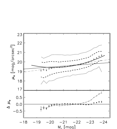
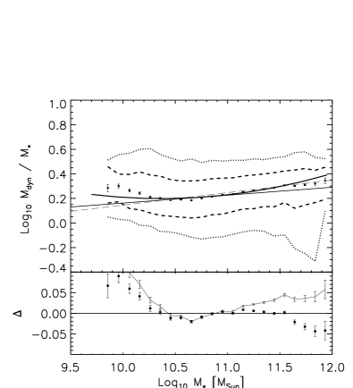
Figure 15: Effect on scaling relations of removing objects with $\sigma<90$ km s^-1. Smooth solid lines show the linear fits to the full sample (taken from previous figures); symbols show the scaling relations when objects with $\sigma<90$ km s^-1 have been removed; dashed and dotted lines enclose 68% and 95% of the objects. Parabolas show the quadratic fits to the symbols.

4 Discussion

We used our own photometric reductions (GALMORPH) of about 6000 early-type galaxies from the SDSS to calibrate corrections to SDSS photometry (equations 3–5) which are most necessary for photometry of extended objects (Figures 5 and 6). We applied these corrections to a larger sample of about 50000 early-types, and then analyzed a number of galaxy scaling relations in the sample. Selection of the sample, which is described in some detail in Section 2, was more conservative than in previous work based on SDSS data.

Small but statistically significant curvature was found for all the relations (Figures 8–12). Table 1 lists the coefficients of best-fitting second-order polynomials which provide a concise way of describing this curvature. The Table also provides the coefficients of linear fits, for comparison. Whereas curvature at large luminosities/stellar masses is expected – BCGs are known to be a special population – some of the scaling relations in our sample show curvature at small masses as well. The critical mass scale is about $M_{*}\approx 3\times 10^{10}\,M_{\odot}$. Whereas we see some evidence from the colors and spectra that objects below this mass scale are of slightly later type (Figures 13 and 14), a visual inspection of the images shows no obvious peculiarities.

Our analysis also showed that the ratio of dynamical to stellar mass increases at large masses (Figure 10); this is a useful constraint on models of early-type galaxy formation. In addition, the $R-\sigma$ and $R-\mu_{e}$ relations were shown to be rather sensitive to selection effects (Figure 12); this matters for analysis of the Fundamental Plane. The question of whether or not the Fundamental Plane is curved or warped is addressed in a companion paper (Hyde & Bernardi 2008). Finally, we showed that seeing biases the scaling relations associated with Petrosian-based quantities (Appendix A), making them ill-suited for precision analyses in large ground-based datasets.

Appendix A Petrosian-related scaling relations are biased by seeing

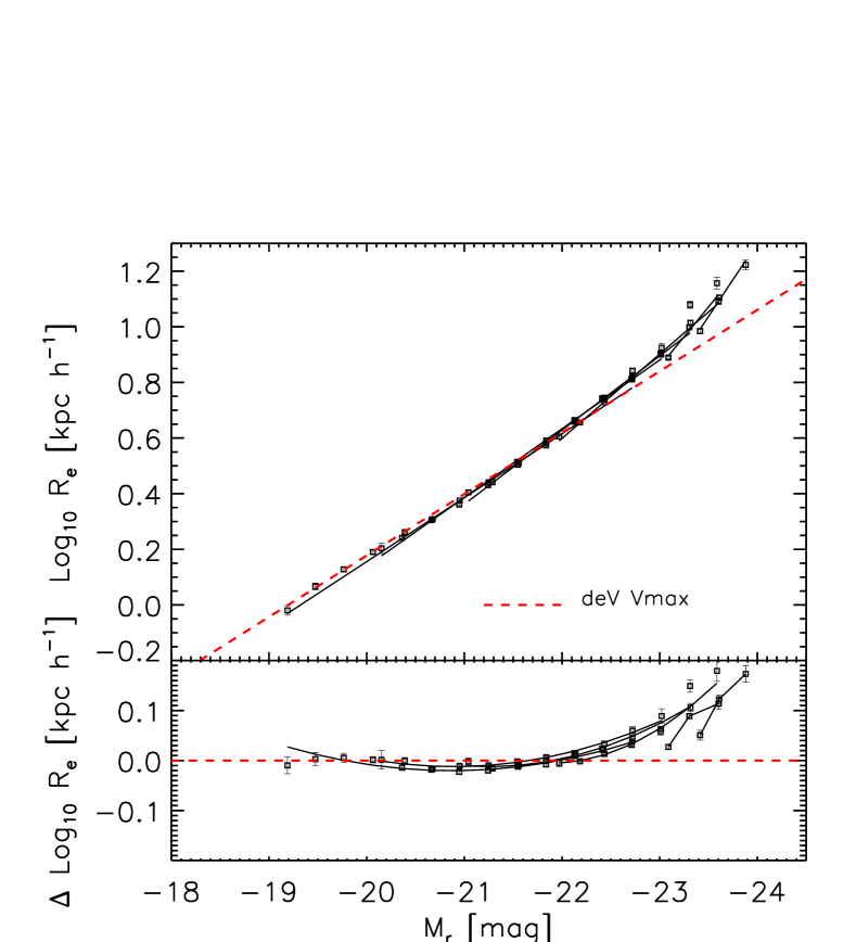
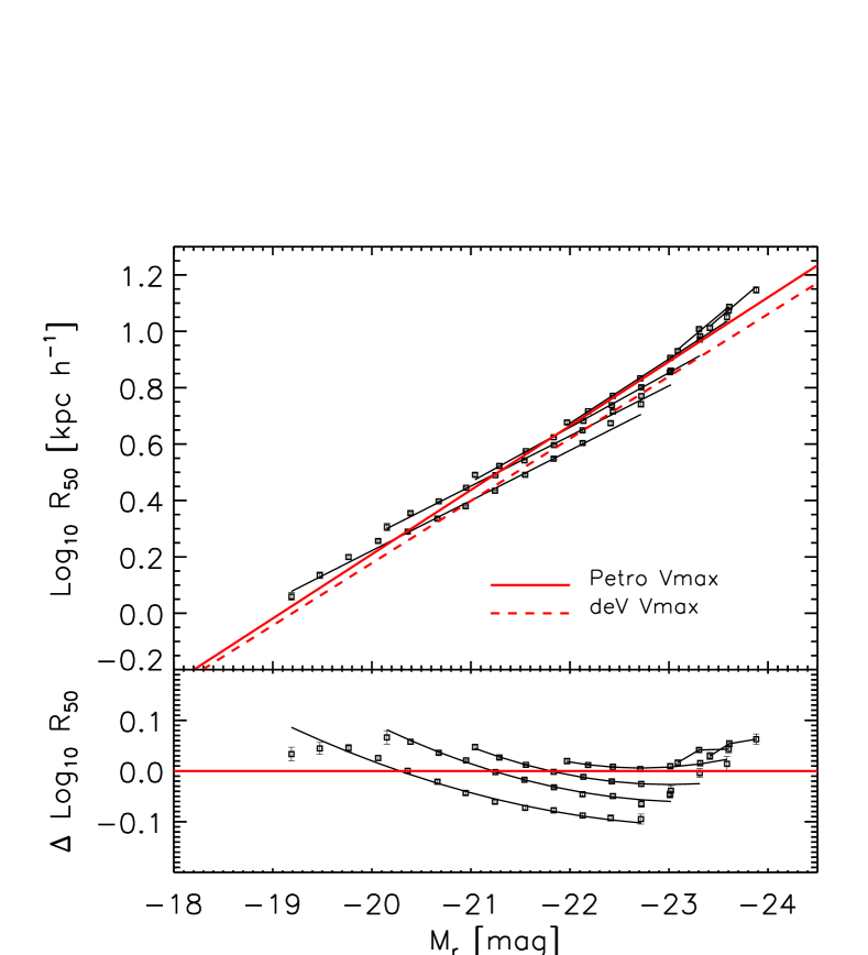
Figure 16: Residuals from the size-luminosity relation in the SDSS $r$-band, derived from deVaucouleur (top) and Petrosian (bottom) quantities; only the former are corrected for the effects of seeing. Different sets of symbols in each panel show this relation at different redshifts; the relation is essentially independent of redshift in the top panel, but the high redshift objects appear to have larger sizes in the bottom panel.

The main text uses sizes and luminosities obtained from fitting deVaucouleur profiles to the images. We chose these over the Petrosian quantities (R50 and petromag) because these latter are not corrected for the effects of seeing. To illustrate that seeing matters, Figure 16 shows the size-luminosity relation in six redshift bins ($0<z\leq 0.07$, $0.07<z\leq 0.1$, $0.1<z\leq 0.13$, $0.15<z\leq 0.18$, $0.22<z\leq 0.25$ and $0.25<z\leq 0.35$, although the luminosities are $k$- and $e$-corrected to $z=0$). The top panel shows deVaucouleur- and bottom shows Petrosian-based results. In the top panel, the size-luminosity relations in the different redshift bins lie on top of one another. In the bottom panel, however, the high redshift relations are offset to larger sizes, suggesting that the Petrosian sizes have been biased high by seeing.

Figure 17: Petrosian concentration as a function of distance from observer for a few bins in (evolution corrected) luminosity ($-21\leq M_{r}\leq-20.5$, $-22\leq M_{r}\leq-21.5$, $-23\leq M_{r}\leq-22.5$, and $-23.5\leq M_{r}\leq-23$) The higher redshift objects have smaller concentrations, because R50 is increasingly affected by seeing.

Figure 17 presents other evidence that seeing matters. It shows the Petrosian concentration (the ratio of the radius which contains 90% of the Petrosian light, to that which contains 50%) as a function of redshift, for a few bins in (evolution-corrected) luminosity ($-21\leq M_{r}\leq-20.5$, $-22\leq M_{r}\leq-21.5$, $-23\leq M_{r}\leq-22.5$, and $-23.5\leq M_{r}\leq-23$). The catalog is apparent magnitude limited, so the most luminous bin extends to highest redshift. At fixed $L$, the higher redshift objects appear to be much less concentrated, but this is not a physical effect: it happens because R50 is increasingly affected by seeing.

In a magnitude limited survey such as the SDSS, the more luminous objects are seen preferentially at larger redshifts. If not accounted for, seeing effects would bias the Petrosian size-luminosity relation (any scaling relations for which size or luminosity matter would also be affected). This can lead to important differences in what one concludes from the data.

For example, in their study of the $R-L$ relation, von der Linden et al. (2007) used Petrosian quantities. They argued that BCGs traced essentially the same $R-L$ relation as the bulk of the early-type galaxy population. This contradicted Lauer et al. (2007) and Bernardi et al. (2007) who found, on the basis of seeing-corrected fits, that the BCG relation was substantially steeper, and used this to draw important conclusions about BCG formation histories. (Steeper relations for BCGs have since also been found by Liu et al. 2008).

The bottom panel of Figure 16 shows that only when one stacks all redshift bins together (and ignores the obvious offset from one redshift bin to the next) does one find a Petrosian $R-L$ relation that is similar to that obtained from seeing-corrected fits; the relation in any one redshift bin is significantly shallower. However, at the highest redshifts, where only the most luminous galaxies contribute, i.e., in the luminosity regime which is most likely to be dominated by BCGs, the $R-L$ relation is indeed substantially steeper. Moreover, its slope becomes similar to that of the (incorrectly!) stacked sample, leading to the conclusion that BCGs have the same slope as the bulk of the population. In effect, using Petrosian quantities without appropriate care for the fact that they are not seeing-corrected, led von der Linden et al. to confusion. For this reason we have not used any Petrosian-based quantities in our analysis, and we caution against their use in general.

This is not to say that we think deVaucouleur-based fits are ideal. One might legitimately ask how the curvature we quantify in the main text changes if we fit to the more general Sersic profile. Fitting two-dimensional Sersic profiles to the SDSS photometry is well beyond the scope of this work. However, in principle, we could have done this approximately as follows. Graham et al. (2005) provide a prescription for transforming from Petrosian to Sersic quantities. So we could have used these transformations as a proxy for actual Sersic fits, and then studied the associated (PSersic?!) scaling relations. In fact, this was done by Desroches et al. (2007). We did not do this here because Figure 16 suggests that, because the Petrosian based quantities have not been seeing-corrected, this would yield biased results.

References

- [\citeauthoryearAdelman-McCarthy et al.2008] Adelman-McCarthy J. K., et al., 2008, ApJS, 175, 297
- [] Almeida, C., Baugh, C. M. & Lacey, C. G., 2007, MNRAS, 376, 1711
- [] Bell E., et al., 2006, ApJ, 652, 270
- [Bernardi et al.(2003)] Bernardi, M., et al. 2003a, AJ, 125, 1817
- [Bernardi et al.(2003)] Bernardi, M., et al. 2003b, AJ, 125, 1849
- [Bernardi et al.(2003)] Bernardi, M., et al. 2003c, AJ, 125, 1866
- [Bernardi et al. 2005] Bernardi M., Sheth R. K., Nichol R. C., Schneider D. P., Brinkmann J., 2005, AJ, 129, 61
- [Bernardi et al.(2006a)] Bernardi, M., Nichol, R. C., Sheth, R. K., Miller, C. J., & Brinkmann, J. 2006a, AJ 131, 1288
- [Bernardi et al.(2006b)] Bernardi, M., et al. 2006b, AJ 131, 2018
- [Bernardi(2007)] Bernardi, M. 2007, AJ 133, 1954
- [Bernardi et al.(2007)] Bernardi, M., Hyde, J. B., Sheth, R. K., Miller, C. J., & Nichol, R. C. 2007, AJ 133, 1741
- [Bernardi et al.(2008)] Bernardi, M., Hyde, J. B., Fritz, A., Sheth, R. K., Gebhardt, K., & Nichol, R. C. 2008, MNRAS in press (arXiv:0809.2602)
- [] Bernardi, M. 2009, MNRAS, submitted
- [Boylan-Kolchin et al.(2005)] Boylan-Kolchin, M., Ma, C.-P., & Quataert, E. 2005, MNRAS 362, 184
- [] Cimatti, A., et al. 2008, A&A, 482, 21
- [\citeauthoryearCiotti, Lanzoni, & Volonteri2007] Ciotti L., Lanzoni B., Volonteri M., 2007, ApJ, 658, 65
- [] De Lucia G., et al., 2006, MNRAS, 366, 499
- [Desroches et al.(2007)] Desroches, L.-B., Quataert, E., Ma, C.-P., West, A. A. 2007, MNRAS 377, 402
- [Gallazzi et al.(2005)] Gallazzi, A., Charlot, S., Brinchmann, J., White, S. D. M., & Tremonti, C. A. 2005, MNRAS 362, 41
- [] Graham, A. et al. 2005, AJ, 130, 1535
- [core] Hopkins, P. F., Lauer, T. R., Cox, T. J., Hernquist, L. & Kormendy, J. 2008a, ApJ, submitted (arXiv:0806.2325)
- [cusp] Hopkins, P. F., Hernquist, L., Cox, T. J., Keres, D., & Wuyts, S. 2008b, ApJ, submitted (arXiv:0807.2868)
- [] Hyde, J. B. & Bernardi, M. 2008, MNRAS, submitted (arXiv:0810.4924)
- [Kauffmann et al.(2003)] Kauffmann, G., et al. 2003, MNRAS 341, 33
- [] Lauer, T. R., et al. 2007, ApJ, 662, 808
- [] Lintott, C. J., Viti, S., Williams, D. A., Rawlings, J. M. C. & Ferreras, I. 2005, MNRAS, 360, 1527
- [] Liu, F. S., Xia, X. Y., Mao, Shude, Wu, Hong & Deng, Z. G. 2008, MNRAS, 385, 23
- [] Malumuth E. M. & Kirshner, R. P. 1981, ApJ, 251, 508
- [] —. 1985, ApJ, 291, 8
- [] Mihos, C. & Hernquist, L. 1993, BAAS, 25, 825
- [] Naab, T., Jesseit, R. & Burkert, A. 2006, MNRAS, 372, 839
- [] Nigoche-Netro, A., Ruelas-Mayorga, A. & Balderas, A. F. 2008, MNRAS, submitted (arXiv:0805.0961)
- [] Oegerle W. R. & Hoessel J. G. 1991, ApJ, 375, 15
- [] Padmanabhan, N. et al. 2004, NewA, 9, 329
- [] Postman M., Lauer T., 1995, ApJ, 440, 28
- [Robertson et al.(2006)] Robertson, B., Cox, T. J., Hernquist, L., Franx, M., Hopkins, P. F., Martini, P., & Springel, V. 2006, ApJ 641, 21
- [] Saglia, R. P., Colless, Matthew, Burstein, David, Davies, Roger L., McMahan, Robert K. & Wegner, Gary 2001, MNRAS, 324, 389
- [] Salviander, S., Shields, G. A., Gebhardt, K., Bernardi, M. & Hyde, J. B. 2008, ApJ, in press (arXiv:0807.3034)
- [] Shen, S. et al. 2003, MNRAS, 343, 978
- [\citeauthoryearStoughton et al.2002] Stoughton C., et al., 2002, AJ, 123, 485
- [] van Dokkum, P. G. et al. 2008, ApJl, 677, 5
- [] von der Linden, A., Best, P. N., Kauffmann, G. & White, S. D. M. 2007, MNRAS, 379, 867
- [] Weinmann, S. M., Kauffmann, G., van den Bosch, F. C., Pasquali, A., McIntosh, D. H., Mo, H., Yang, X, & Guo, Y. 2008, MNRAS, submitted (arXiv:0809.2283)
- [] Zaritsky, D., Gonzales, A. H. & Zabludoff A. 2006, 638, 725