The 2dF-SDSS LRG and QSO Survey: The spectroscopic QSO catalogue.

Abstract

We present the final spectroscopic QSO catalogue from the 2dF-SDSS LRG and QSO (2SLAQ) Survey. This is a deep, $18<g<21.85$ (extinction corrected), sample aimed at probing in detail the faint end of the broad line AGN luminosity distribution at $z\hbox{\hbox to0.0pt{\raise 1.82986pt\hbox{$<$}\hss}\lower 2.79857pt\hbox{$\sim$}}2.6$. The candidate QSOs were selected from SDSS photometry and observed spectroscopically with the 2dF spectrograph on the Anglo-Australian Telescope. This sample covers an area of 191.9 deg² and contains new spectra of 16326 objects, of which 8764 are QSOs, and 7623 are newly discovered (the remainder were previously identified by the 2QZ and SDSS surveys). The full QSO sample (including objects previously observed in the SDSS and 2QZ surveys) contains 12702 QSOs. The new 2SLAQ spectroscopic data set also contains 2343 Galactic stars, including 362 white dwarfs, and 2924 narrow emission line galaxies with a median redshift of $z=0.22$.

We present detailed completeness estimates for the survey, based on modelling of QSO colours, including host galaxy contributions. This calculation shows that at $g\simeq 21.85$ QSO colours are significantly affected by the presence of a host galaxy up to redshift $z\sim 1$ in the SDSS $ugriz$ bands. In particular we see a significant reddening of the objects in $g-i$ towards fainter $g$-band magnitudes. This reddening is consistent with the QSO host galaxies being dominated by a stellar population of age at least $2-3$ Gyr.

The full catalogue, including completeness estimates, is available on-line at http://www.2slaq.info/.

1 Introduction

The last decade has seen the coming of age of extremely high multiplex fibre spectroscopy, as implemented by the 2-degree Field (2dF) instrument [Lewis et al. 2002] and the Sloan Digital Sky Survey (SDSS; York et al. 2000). These new facilities have allowed order of magnitude increases in sample sizes over the previous generation of surveys. The 2dF QSO Redshift Survey (2QZ; Croom et al. 2001a; 2004) and the SDSS QSO survey (Schneider et al. 2007) have allowed precise measurement of the evolution of QSOs (e.g. Boyle et al. 2000; Croom et al. 2004; Richards et al. 2006), QSO clustering (e.g. Croom et al. 2001b; Croom et al. 2005; Shen et al. 2007), spectral properties (e.g. Croom et al. 2002; Corbett et al. 2003; Vanden Berk et al. 2001; Richards et al. 2002a) and a range of other significant results. The published sample sizes ($\sim 25000$ QSOs in 2QZ; $\sim 80000$ QSOs in SDSS) are large enough that in many cases measurements are now limited by systematic uncertainties rather than random errors.

However, one of the important limitations of the 2QZ and SDSS surveys are their relative depths. The SDSS QSO survey is limited to $i=19.1$, or $i=20.2$ for the high redshift sample [Richards et al. 2002b], which does not reach the break in the QSO luminosity function. 2QZ is somewhat deeper, limited in the bluer $b_{\rm J}$-band to $b_{\rm J}<20.85$. The 2QZ clearly shows the break in the QSO luminosity function (LF), typically reaching $\sim 1$ mag fainter than the break at $z<2$. The observed break in the LF is a gradual flattening towards faint magnitudes; as a result the constraints from the 2QZ on the actual slope of the faint end are fairly uncertain, as evidenced by the difference between the results from the first release (Boyle et al. 2000) and the final release (Croom et al. 2004; C04). In comparison, X-ray surveys, in particular using Chandra (e.g. Giacconi et al. 2002; Alexander et al. 2003) and XMM-Newton (e.g. Hasinger et al. 2001; Worsley et al. 2004; Barcons et al. 2007), reach to fainter depths, but over a much smaller area. The largest samples contain $\sim 1000$ objects over a few square degrees. These surveys have demonstrated that the pure luminosity evolution that appears to model the evolution of the most extensive optical samples (e.g. 2QZ, SDSS) fails to trace the evolution of the faint AGN populations at $L<L^{*}$. It now appears that the activity in faint AGN peaks at a lower redshift than that of more luminous AGN (e.g. Hasinger et al 2005); this process has been described as AGN downsizing (e.g. Barger et al. 2005). Whether the downsizing is due to lower mass black holes being more active at low redshift (e.g. Heckman et al. 2004) or massive black holes at lower rates of accretion (e.g. Babic et al., 2007) remains unclear. Both effects are likely to play a role.

Substantial advances have been made in the theoretical understanding of AGN formation and the connection to galaxy formation (e.g. Hopkins et al. 2005a). This work has been largely driven by the observational evidence that most massive galaxies with bulges contain super-massive BHs (SMBHs) (e.g. Tremaine et al. 2002). SMBH accretion is thought to be triggered (at least for moderate to high luminosity AGN) by the merger of gas rich galaxies; while the timescale for the merger may be as long as $\sim 1$Gyr, during the majority of this time the accretion is obscured from view. It is only when the AGN finally expels the surrounding gas and dust that it shines like a quasar for a brief period ($\sim 100$Myr), before exhausting its fuel supply (e.g. Di Matteo et al. 2005). This feedback of the AGN into the host also heats (and possibly expels) the gas in the galaxy, which suppresses star formation leading to “red and dead” ellipticals or bulges. These models match a number of previous observations and predict that the faint end of the QSO luminosity function is largely comprised of higher mass BHs at lower accretion rates (i.e. below their peak luminosity) [Hopkins et al. 2005b].

The 2dF SDSS LRG and QSO (2SLAQ) Survey was designed to survey optically faint AGN/QSOs within a sufficiently large volume to obtain robust measurements of both the luminosity function and QSO clustering. Throughout this paper we will use the term QSO to refer to any broad line (type 1) AGN, irrespective of luminosity. The QSO portion of the survey shared fibres with a related program to target luminous red galaxies (LRGs) at $z\simeq 0.4-0.7$ (Cannon et al. 2006). Both the LRGs and QSOs were selected from single epoch SDSS imaging data, and then observed spectroscopically with the 2-degree Field (2dF) instrument at the Anglo-Australian Telescope (AAT). The 2SLAQ QSO sample has already produced a preliminary QSO luminosity function (Richards et al. 2005; R05), measured the clustering of QSOs as a function of luminosity (da Angela et al. 2008) and studied the distribution of QSO broad line widths (Fine et al. 2008). In this paper we present the final spectroscopic QSO catalogue of the 2SLAQ sample. We then carry out a detailed analysis of the survey completeness. The analysis of the QSO luminosity function from the final 2SLAQ sample is presented in a companion paper (Croom et al. in prep).

In Section 2 we discuss the selection of QSO candidates from the SDSS imaging data. This has largely been described by R05, but is summarized here for completeness. In Section 3 we present the spectroscopic observations, and in Section 4 we describe the composition and quality of the resulting catalogue. Section 5 contains our detailed completeness analysis. We summarize our results in Section 6. Throughout this paper we will assume a cosmology with $H_{0}=70$km s^-1Mpc^-1, $\Omega_{\rm m}=0.3$ and $\Omega_{\Lambda}=0.7$.

2 Imaging data and QSO selection

2.1 The SDSS imaging data

The photometric measurements used as the basis for our catalogue are drawn from the Data Release 1 (DR1) processing (Stoughton et al. 2002; Abazajian et al. 2003) of the SDSS imaging data. The astrometric precision at the faint limit of the survey is $\sim 0.1$ arcsec [Pier et al. 2003]. The SDSS data are taken in five photometric pass-bands ($ugriz$; Fukugita et al. 1996) using a large format CCD camera [Gunn et al. 1998] on a special-purpose 2.5-m telescope (Gunn et al. 2006). The regions covered by the 2SLAQ survey were complete in DR1, so no further updates to more recent data releases are required. Except where otherwise stated, all SDSS magnitudes discussed herein are “asinh” point-spread-function (PSF) magnitudes [Lupton, Gunn, & Szalay 1999] on the SDSS pseudo–AB magnitude system [Oke & Gunn 1983] that have been dereddened for Galactic extinction according to the model of Schlegel, Finkbeiner & Davis (1998). The SDSS Quasar Survey [Schneider et al. 2007] extends to $i=19.1$ for $z<3$ and $i=20.2$ for $z>3$; our work herein explores the $z<3$ regime to $g=21.85$ ($i\sim 21.63$, based on the median colours of SDSS QSOs, e.g. Richards et al. 2001). At the faint limit of the 2SLAQ sample ($21.75<g<21.85$), the photometric errors are typically $\Delta u=0.20$, $\Delta g=0.07$, $\Delta r=0.08$, $\Delta i=0.11$, $\Delta z=0.33$.

2.2 Sample selection

2.2.1 Preliminary sample restrictions

Our quasar candidate sample was drawn from 10 SDSS imaging runs. Due to the slightly poorer image quality in the 6th row of CCDs in the SDSS camera we did not include these data. Thus the 2SLAQ survey regions are $2^{\circ}$ wide rather than the usual $2^{\circ}.5$ for an SDSS imaging run. We rejected any objects that met the “fatal” or “non-fatal” error definitions of the SDSS quasar target selection [Richards et al. 2002a]. Although our survey covers the southern equatorial Stripe 82 region which has been scanned multiple times [Adelman-McCarthy et al. 2008], the co-added data (Annis et al. 2006) were not available at the time of our spectroscopic observations and so single scan data were used.

We apply a limit to the (extinction corrected) $i$-band PSF magnitude of $i<22.0$ and $\sigma_{i}<0.2$. We also placed restrictions on the errors in each of the other four bands: $\sigma_{u}<0.4$, $\sigma_{g}<0.13$, $\sigma_{r}<0.13$ and $\sigma_{z}<0.6$. Note that this selection of error constraints effectively limits the redshift to less than 3, as the Ly$\alpha$ forest suppresses the $u$ flux at higher redshifts.

2.2.2 Low redshift colour cuts

Based on spectroscopic identifications from SDSS and 2QZ of this initial set of objects, we implement additional colour cuts that are designed to select faint UV-excess QSOs with high efficiency and completeness at redshifts $z\hbox{\hbox to0.0pt{\raise 1.82986pt\hbox{$<$}\hss}\lower 2.79857pt\hbox{$\sim$}}2.6$. An analysis of the completeness of the selection algorithm is given as a function of redshift and magnitude in Section 5.2.

We reject hot white dwarfs using the following cuts, independent of magnitude. Specifically, we rejected objects that satisfy the condition: A AND ((B AND C AND D) OR E), where the letters refer to the cuts:

$$\begin{array}[]{rrcccl}{\rm A})&-1.0&<&u-g&<&0.8\\ {\rm B})&-0.8&<&g-r&<&0.0\\ {\rm C})&-0.6&<&r-i&<&-0.1\\ {\rm D})&-1.0&<&i-z&<&-0.1\\ {\rm E})&-1.5&<&g-i&<&-0.3.\end{array}$$ (6)

These constraints are similar to the white dwarf cut applied by Richards et al. (2002a; their Eq. 2) except for the added cut with respect to the $g-i$ colour.

Figure 1: The UKST $b_{\rm J}$ (Maddox & Hewett 2006) and SDSS $g$ transmission curves (detector quantum efficiency) for airmass of 1. Normalization is such that $\int S_{\lambda}{\rm d}\lambda/\lambda=1$. This is a corrected version of the same plot shown by R05, in which the conversion from energy to photon efficiency for the $b_{\rm J}$ response was incorrect.

To efficiently target both bright and faint targets we use different colour cuts as a function of $g$-band magnitude. The bright sample is restricted to $18.0<g<21.15$ and is designed to allow for overlap with previous SDSS and 2dF spectroscopic observations. The faint sample has $21.15\leq g<21.85$ and probes roughly one magnitude deeper than 2QZ. These cuts are made in $g$, rather than the $i$-band that the SDSS quasar survey uses, since we are concentrating on UV-excess quasars and would like to facilitate comparison with the results from the $b_{\rm J}$-based 2QZ. At this depth an $i$-band limited sample selected from single epoch SDSS data would also contain substantial stellar contamination. The combination of the $g<21.85$ and $i<22.0$ cuts will exclude objects bluer than $\alpha_{\nu}=+0.3\;(f_{\nu}\propto\nu^{\alpha})$; however, objects this blue are exceedingly rare ($>3\sigma$ deviations from the observed QSO spectral slope distribution; Richards et al 2006). As pointed out by R05, the $b_{\rm J}$ and $g$ bands are almost equivalent, with a mean $(g-b_{\rm J})=-0.045$ found for QSOs in common between the SDSS and 2QZ. We note that the relative transmission curves plotted in R05 (their Fig. 6) were in error (the energy to photon conversion was reversed). We plot the correct comparison in Fig. 1.

In general, we would prefer to avoid a morphology-based cut since we do not want to exclude low-$z$ quasars and because our selection extends beyond the magnitude limits at which the SDSS’s star/galaxy separation breaks down. However, Scranton et al. (2002) have developed a Bayesian star-galaxy classifier that is robust to $r\sim 22$. As a result, in addition to straight colour-cuts, we also apply some colour restrictions on objects with high $r$-band galaxy probability (referred to below as “galprob”) according to Scranton et al. (2002) in an attempt to remove contamination from narrow emission line galaxies (NELGs; i.e. blue star-forming galaxies) from our target list.

Bright sample objects are those with $18.0<g<21.15$ and that meet the following conditions

$$\begin{array}[]{rcclcccll}{\rm A})&u-g&<&0.8&{\rm AND}&g-r&<&0.6&{\rm AND}\\ &r-i&<&0.6&&&&&\\ {\rm B})&u-g&>&0.6&{\rm AND}&g-i&>&0.2&\\ {\rm C})&u-g&>&0.45&{\rm AND}&g-i&>&0.35&\\ {\rm D})&{\rm galprob}&>&0.99&{\rm AND}&u-g&>&0.2&{\rm AND}\\ &g-r&>&0.25&{\rm AND}&r-i&<&0.3&\\ {\rm E})&{\rm galprob}&>&0.99&{\rm AND}&u-g&>&0.45.&\end{array}$$ (14)

in the combination A AND (NOT B) AND (NOT C) AND (NOT D) AND (NOT E), where cut A selects UVX objects, cuts B and C eliminate faint F-stars whose metallicity and errors push them blueward into the quasar regime, and cuts D and E remove NELGs that appear extended in the $r$ band. Among the bright sample objects, those with $g>20.5$ were given priority in terms of fibre assignment (see Section 3.2).

Faint sample objects are those with $21.15\leq g<21.85$ and that meet the following conditions

$$\begin{array}[]{rcclcccll}{\rm A})&u-g&<&0.8&{\rm AND}&g-r&<&0.5&{\rm AND}\\ &r-i&<&0.6&&&&&\\ {\rm B})&u-g&>&0.5&{\rm AND}&g-i&>&0.15\\ {\rm C})&u-g&>&0.4&{\rm AND}&g-i&>&0.3\\ {\rm D})&u-g&>&0.2&{\rm AND}&g-i&>&0.45\\ {\rm E})&{\rm galprob}&>&0.99&{\rm AND}&g-r&>&0.3.\end{array}$$ (21)

in the combination A AND (NOT B) AND (NOT C) AND (NOT D) AND (NOT E), where cut A selects UVX objects, cuts B, C and D eliminate faint F-stars whose metallicity and errors push them blueward into the quasar regime, and cut E removes NELGs. These faint cuts are more restrictive than the bright cuts to avoid significant contamination from main sequence stars that will enter the sample as a result of larger errors at fainter magnitudes. The low redshift colour cuts ($u-g$ and $g-i$) are shown in Fig. 12 (see also Fig. 1 of R05).

2.2.3 High redshift colour cuts

In addition to the main low redshift ($z\hbox{\hbox to0.0pt{\raise 1.82986pt\hbox{$<$}\hss}\lower 2.79857pt\hbox{$\sim$}}2.6$) sample described above, we also target a sample of higher redshift QSO candidates, analogous to the high redshift sample selected in the main SDSS QSO survey which selected QSOs up to $z\simeq 5.4$ at $i<20.2$ (Richards et al. 2002a). The 2SLAQ high redshift sample was limited to $i<21.0$ and an additional constraint that $\sigma_{z}<0.4$ was applied to the $z$-band photometry. We then selected candidates in three redshift intervals. QSO candidates at redshift $\simeq 3.0-3.5$ satisfied the following cuts:

$$\begin{array}[]{cclc}\sigma_{r}&<&0.13&{\rm AND}\\ u&>&20.6&{\rm AND}\\ u-g&>&1.5&{\rm AND}\\ g-r&<&1.2&{\rm AND}\\ r-i&<&0.3&{\rm AND}\\ i-z&>&-1.0&{\rm AND}\\ g-r&<&0.44(u-g)-0.76.\\ \end{array}$$ (29)

For the redshift range $\simeq 3.5-4.5$ this selection becomes

$$\begin{array}[]{ccclccclc}{\rm A})&\sigma_{r}&<&0.2&\\ {\rm B})&u-g&>&1.5&OR&u&>&20.6\\ {\rm C})&g-r&>&0.7&\\ {\rm D})&g-r&>&2.8&OR&r-i&<&0.44(g-r)-0.558\\ {\rm E})&i-z&<&0.25&{\rm AND}&i-z&>&-1.0,\\ \end{array}$$ (35)

in the combination A AND B AND C AND D AND E. For the redshifts above $\simeq 4.5$ we use

$$\begin{array}[]{cclc}u&>&21.5&{\rm AND}\\ g&>&21.0&{\rm AND}\\ r-i&>&0.6&{\rm AND}\\ i-z&>&-1.0&{\rm AND}\\ i-z&<&0.52(r-i)-0.762.\\ \end{array}$$ (41)

These samples have a high degree of contamination from the stellar locus due to photometric errors. These candidates were therefore targeted at a lower priority than the main low redshift sample, and we do not present a detailed analysis of completeness for the high redshift sample.

2.3 Survey area

Table 1: Coordinates of the 2SLAQ survey regions.

2SLAQ	RA (J2000)		Dec (J2000)
Region	min	max	min	max
a	123.0	144.0	-1.259	0.840
b	150.0	168.0	-1.259	0.840
c	185.0	193.0	-1.259	0.840
d	197.0	214.0	-1.259	0.840
e	218.0	230.0	-1.259	0.840
s	309.0	59.70	-1.259	0.840

Table 2: SDSS imaging runs used for 2SLAQ target selection. We list the run number, modified Julian date (MJD) of observation and the 2SLAQ regions that each run contributes to. Note that runs can contribute to more than one 2SLAQ region.

SDSS run	MJD	2SLAQ regions
752	51258	c, d, e
756	51259	a, b, c, d, e
1239	51607	a
2141	51962	b
2583	52172	s
2659	52197	s
2662	52197	s
2738	52234	s
3325	52522	s
3388	52558	s

The survey was targeted along the two equatorial regions from the SDSS imaging data. In the North Galactic Cap, we selected five disjoint regions along $\delta\simeq 0^{\circ}$ which contain the best quality imaging data. These are denoted as regions a, b, c, d, e, as listed in Table LABEL:tab:surv_regions. In the South Galactic Cap we targeted a single contiguous region, denoted as s. The 10 SDSS imaging runs used are listed in Table LABEL:tab:runs, along with the 2SLAQ regions to which they contribute. The 2SLAQ area completely overlaps with the brighter SDSS QSO survey (e.g. Schneider et al. 2007). There is partial overlap with the 2QZ (C04) in the North Galactic Cap, with the 2QZ covering the RA range $148^{\circ}<\alpha_{\rm J2000}<223^{\circ}$.

3 Spectroscopic observations

3.1 Instrumental setup

Spectroscopic observations of the input catalogue were made with the 2-degree Field (2dF) instrument at the Anglo-Australian Telescope [Lewis et al. 2002]. The 2dF instrument is a multi-fibre spectrograph which can obtain simultaneous spectra of up to 400 objects over a $2^{\circ}$ diameter field of view, and is located at the prime focus of the telescope. Fibres are robotically positioned within the field of view and are fed to two identical spectrographs (200 fibres each). Two field plates and a tumbling system allow one field to be observed while a second is being configured, reducing down-time between fields to a minimum. The spectrographs each contain a Tektronix $1024\times 1024$ CCD with 24 $\mu$m pixels.

Observations of QSOs and LRGs were combined by using 200 fibres for each sample and sending these to separate spectrographs. QSO targets were sent to spectrograph 1 which contained a low resolution 300B grating with a central wavelength of 5800Å. LRG targets were directed to spectrograph 2 with a higher resolution 600V grating centred at 6150Å (see Cannon et al. 2006 for further details of the LRG sample). The 300B grating produces a dispersion of 4.3Å pixel^-1, giving an instrumental resolution of 9Å. The spectra covered the wavelength range 3700–7900Å.

3.2 Target configuration and priority

Table 3: Configuration priorities for 2SLAQ targets. 9 is the highest priority, while 1 is the lowest.

Sample	Priority
Guide stars	9
LRG (main) random	8
LRG (main) remainder	7
QSOs ($g>20.5$) random	6
QSOs ($g>20.5$) remainder	5
LRG(extras)+hi-z QSOs	4
QSOs ($g<20.5$)	3
previously observed	1

The 2dF CONFIGURE program [Shortridge & Ramage 2003] was used to allocate specific fibres to objects. This software takes an input list of prioritized positions (including guide fibres and target positions) and through an iterative scheme allocates fibres, producing a second file which is passed to the control software for the 2dF robotic positioner. For the 2SLAQ observing program, minor modifications to the CONFIGURE software were made to allow i) fibres from different spectrographs to be allocated to different samples, ii) different central wavelengths for each spectrograph. We also carried out a detailed analysis of the spatial variation of configured target density across the 2dF field. This showed that the algorithm could, in certain circumstances, impart considerable structure on the distribution of targets. The main effects seen were a deficit of objects near the centre of the field ($<0.25^{\circ}$ radius) in high density fields (where the number of targets is greater than the number of fibres) and systematics related to the ordering of targets. To address these issues, the targets were randomized and randomly re-sampled so that so that the highest priority targets had a surface density of 70 deg^-2. We note that these issues have since been fully addressed by Mizarksi et al. (2006) using a simulated annealing algorithm; however, 2SLAQ observations were carried out prior to this work.

Our most important targets were given higher priority in the fibre configuration process. These priorities are summarized in Table 3. LRGs were given highest priority because they have a lower surface density than the QSO candidates. Our highest priority QSO targets had $g>20.5$ and were given a priority of 6. The surface density of these targets was significantly higher than the $\sim 70$ deg^-2 that can be configured with the available fibres and so were randomly re-sampled. The remaining $g>20.5$ QSOs (not selected in the random sampling) had their priority set to 5. The high redshift QSO candidates had their priorities set to 4, and the bright QSO candidates ($g<20.5$) had priority of 3. If a 2SLAQ selected source already had a high quality spectroscopic observation from either 2QZ or SDSS its priority was set to 1 (lowest on a scale of $1-9$) in the 2dF configuration (i.e. it was observed only if no other target was available).

3.3 Tiling of 2dF fields

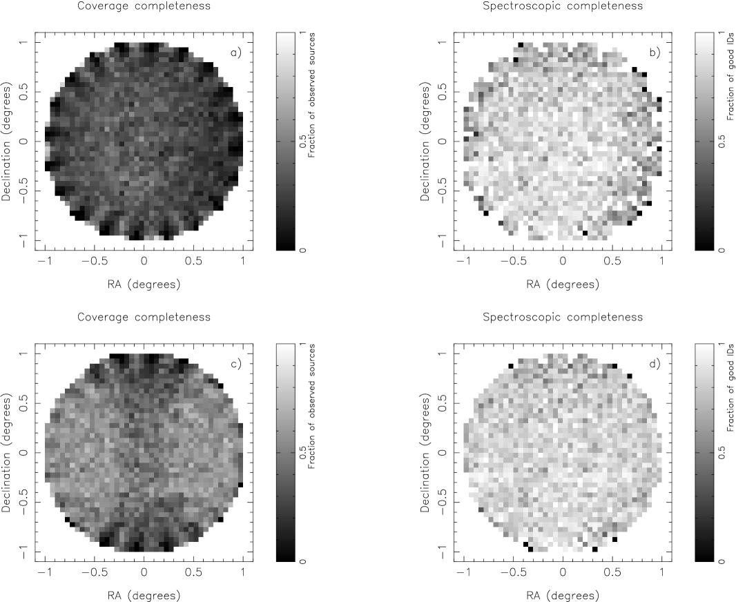
Figure 2: 2SLAQ survey completeness as a function of 2dF field position. a) Average coverage completeness within individual 2dF pointings. Note the small triangular regions at the edge of the field which are inaccessible due to alternating blocks of 10 fibres going to the LRG sample. There is also a slight deficit of observed targets on the right hand side of the field, due to the sky fibres preferentially coming from that side of the field. This is compensated for by overlapping fields. b) Average spectroscopic completeness for individual 2dF pointings. A small decline is visible towards the field edge (see Fig. 3). c) Coverage completeness for all objects within a 2dF field radius (allowing for overlaps). Regions of increased completeness due to overlapping fields can be seen to the East and West edges of the field. d) Spectroscopic completeness for all objects within a 2dF field radius (allowing for overlaps). This distribution is quite uniform over the entire field.

Table 4: 2SLAQ observed objects which are outside of the nominal survey limits bounded by the intersection of $1.05^{\circ}$ radius 2dF fields of view.

Name	RA (J2000)	Dec. (J2000)
	(deg)	(deg)
J005128.22$+$004447.8	12.867619	0.746637
J010159.56$+$004820.2	15.498189	0.805634
J010423.79$+$004029.8	16.099131	0.674965
J022526.32$-$011434.3	36.359680	-1.242874
J081233.10$+$004643.0	123.137909	0.778604
J081238.23$+$004713.2	123.159286	0.786992
J081938.22$-$011052.6	124.909256	-1.181273
J100705.00$-$010904.9	151.770844	-1.151354
J123158.37$+$004635.6	187.993195	0.776566
J123448.89$+$004752.3	188.703705	0.797856
J134054.18$+$004911.9	205.225769	0.819972
J143313.87$-$011501.2	218.307800	-1.250338
J143620.20$+$004529.6	219.084152	0.758220
J143922.06$-$011215.0	219.841934	-1.204170
J144007.84$+$004156.2	220.032654	0.698939
J211844.76$+$003134.4	319.686523	0.526249
J211955.31$+$004301.6	319.980469	0.717123
J212129.68$+$004827.1	320.373688	0.807553
J214859.57$+$004439.5	327.248230	0.744307

Given the geometry of the imaging area (strips between 10^∘ and 110^∘ long, which are all $2^{\circ}$ wide), it was sensible to employ a simple tiling pattern to cover the 2SLAQ regions. Each circular 2dF field was spaced along the strip at intervals of $1.2^{\circ}$ in RA. In some cases field centres were shifted slightly to optimize their positions (e.g. at the end of survey regions). Some of the first fields observed (February - April 2003) had a smaller spacing of $1^{\circ}$. The 1.2^∘ spacing produced a near optimal balance between coverage and completeness for both the QSOs and LRGs. This approach also provides some overlap between adjacent fields. The 2dF field of view has a radius of $1.05^{\circ}$. For most observations, configured objects were constrained to lie within a circle of exactly $1.05^{\circ}$ radius; however, early observations did not apply this constraint (February – September 2003). As a result, 19 2SLAQ objects (including 10 good quality QSOs) were observed marginally outside the nominal survey region bounded by the intersection of all the observed fields each with radius $1.05^{\circ}$. This can be caused by effects such as atmospheric refraction which distorts the field of view at high airmass. These are included in the catalogue, but excluded in several of the analyses below; the names of these sources are given in Table 4.

Figure 3: 2SLAQ survey completeness as a function of radius from 2dF field centres averaged over all 2SLAQ fields. a) Coverage (filled circles) and spectroscopic (open circles) completeness within individual 2dF pointings. A clear decline towards the field edge is seen in both cases. The solid and dashed lines show the mean coverage and spectroscopic completeness respectively within a radius of $0.5^{\circ}$. b) As for a), but calculated for all objects within a 2dF field radius (allowing for overlaps). The depression at less than $\sim 0.3^{\circ}$ in the coverage (filled points) is because the overlapping fields do not quite reach to the middle of the adjacent field (c.f. Fig. 2).

In order to maximize the yield from overlapping fields, sequences of alternating fields were generally observed first, with the interleaved overlapping fields observed in a second pass. On this second pass, all targets which obtained high quality identifications (quality 1; see Section 3.6 below) from previous observations were given the lowest priority (priority 1), so that a minimal number of objects with acceptable spectroscopic data were repeated. Even allowing for this, 3317 objects have repeat observations. Approximately half of these were because the original spectrum was low quality. The other half were repeated because there was no higher priority target accessible. These repeated spectra are useful in making internal checks of completeness and consistency.

There are also a number of physical constraints on the configuration of 2dF fields. In the 2SLAQ survey the most apparent of these is that fibres are arranged around the edge of the field plates in blocks of 10. These blocks of 10 fibres go to alternating spectrographs, such that there is a triangular region directly in front of each fibre block going to spectrograph 2 that fibres from spectrograph 1 cannot access. This is because 2dF fibres are limited to a maximum off-radial angle of $14^{\circ}$. The 20 small inaccessible triangles amount to a total area of 0.43 deg². As a number of different samples are configured together in each field, the distribution of other targets also influences the angular selection function within 2dF fields. The main QSO sample was given lower priority than the main LRG sample, so great care needs to be taken determining statistics (e.g. clustering) which depend on the angular distribution of QSOs (see da Angela et al. 2008). In addition, 2dF fibres cannot be positioned closer than $\sim 30$ arcsec, which can reduce the number of close pairs on these angular scales. Finally, 20 fibres were allocated to sky positions. Each 2dF spectrograph CCD takes data from 200 fibres. The sky positions were allocated to fibres that lay in the central 100 fibres on the spectrograph CCD (which predominantly come from the western side of the 2dF field). This region on the CCD has the best spectral and spatial PSF, allowing PSF mapping and convolution to improve sky subtraction if required [Willis et al. 2001].

The influence of these varied effects is displayed in Fig. 2. The unreachable triangular regions near the edge of the field are clearly visible in Fig. 2a, while when overlaps are considered (Fig. 2c) these features are only seen at the very top and bottom of the field. Radial variations in spectroscopic completeness are also visible (Fig. 2b; Fig. 3). Both coverage and spectroscopic completeness gradients are visible, but these are much less pronounced when the overlaps between fields are taken into account.

3.4 2dF observations

2SLAQ observations were carried out over a period February 2003 to August 2005, using a total of 89 nights of AAT time. The fiducial exposure time for each field was 4 hours. Due to the effects of differential spatial atmospheric refraction across the 2 degree field of view, a single field could not be observed for more than $\sim 2$ hours at a time (and significantly less if observed at high airmass), so a field would typically be observed over 2 nights, with 4x1800s exposures being taken each night.

Data reduction and quality assessment at the telescope enabled determination of whether the nominal spectroscopic completeness limit for QSO candidates had been obtained ($>80$ per cent quality 1 IDs; see Section 3.6 below). Further observations were taken if this limit was not obtained, usually because of poor weather. This analysis allowed us to identify those objects which had sufficient $S/N$ for a good identification in only the first 2 hours of observing a field. Any fibres on such objects were re-allocated to previously unallocated targets (for observations in 2004 and 2005 only). This was done by setting any object with a good quality ID to have priority=1 (the lowest). Then the CONFIGURE program was re-run, but with the fibre allocations to objects which still needed further observation locked in place. This was particularly useful in quickly removing narrow emission line galaxies (NELGs) which are often clearly identifiable in only 2 hours of observation. Information on the observed 2SLAQ fields is presented in Table LABEL:tab:fields1. This lists the number of objects observed in each field, the number of QSOs and the fraction of good quality IDs. These quantities are listed for the primary fibre allocation; i.e. the sources targeted in the first night’s observation of each field. All of these targets will have the full exposure time or have high quality IDs in shorter exposure times. We also list the numbers and completeness for all the targets in each field, including those only observed on the second (or subsequent) night. In principle, these could have lower completeness, as they have had shorter than average total exposure times.

3.5 Data reduction

The data from the 2dF spectrographs were reduced using the 2DFDR data reduction software [Bailey et al. 2004]. Observations of a typical field contain a fibre flat field, a calibration arc, $4\times 1800$s object frames and a final calibration arc. The fibre flat field frame is used to trace the positions of the fibres across the CCD and determine the spatial profiles of the spectra for optimal extraction, as well as to flat field the spectra to remove fibre-to-fibre variations in spectral response. For the object frames, fibre throughput is calibrated using the flux in a number of strong night sky lines and a median sky spectrum, scaled by the strong sky lines, is then subtracted. The object frames are combined using a variance weighting and an additional weight (per frame) based on the mean flux in each frame. This accounts for variable seeing, cloud cover etc. Various modifications were made to the 2DFDR software for the 2SLAQ project. These include improvements to allow combining of data for the same object taken in different configurations and providing more robust methods of weighting frames. Improvements were also made to the wavelength calibration and flat fielding. We note that the spectra are not spectrophotometrically calibrated.

Data were reduced on the night of observation by team members present at the telescope. This operational approach has the advantage of pseudo-real-time quality control of the data. If the required spectroscopic completeness was not achieved (80 per cent quality 1 identifications; see Section 3.6 below), the exposure time was extended.

3.6 Spectroscopic identification

In most cases spectroscopic identification was also performed on the night of observation at the telescope. This enabled targets which had sufficient $S/N$ for a good (quality 1) identification to be removed from the configuration of the given field on subsequent nights; the newly available fibres were then allocated to other targets. Identification of QSO candidates was carried out in a two stage process. First the automated identification software, AUTOZ, was used to determine the redshift and type (e.g. QSO, star etc.) of the object. These automated identifications were checked using the 2DFEMLINES software, which allows users to check the identifications by eye and interactively adjust the identification if required. Both AUTOZ and 2DFEMLINES were written for the 2QZ; details of the code are given by Croom et al. (2001b) and C04. Briefly, AUTOZ relies on a $\chi^{2}$-minimization technique, comparing an observed spectrum to a number of (redshifted) template spectra. Based on this fitting, the spectra are classified into six categories:

QSO:	Broad ($>1000\,$km s-1) emission lines.
NELG:	Narrow ($<1000\,$km s-1) emission lines only.
gal:	Galaxy absorption features only.
star:	Stellar absorption features at $z=0$.
cont:	No emission or absorption features (High S/N).
??:	No emission or absorption features (Low S/N).

A broad absorption line (BAL) QSO template was included, and when verified by eye, BAL QSOs were labelled as “QSO(BAL)” in the final catalogue. Of 2SLAQ QSOs above $z=1.5$, where C IV is visible in the observed spectrum, 171/4591 (3.7 per cent) are classified as BALs. This is a lower limit to the total BAL fraction as we have not performed a consistent and quantitative analysis for BALs [e.g. using the BALnicity index of Weymann et al.(1991)]. As a part of the identification process, each spectrum is assigned a quality for the identification and redshift as follows:

Quality 1:	High-quality identification or redshift.
Quality 2:	Poor-quality identification or redshift.
Quality 3:	No identification or redshift assignment.

The quality flag was determined independently for the identification and redshift of an object. For example, a quality 1 QSO identification could have a quality 1 or 2 redshift. A quality 1 identification is assigned if multiple spectral features are seen. QSOs with only a strong broad Mg II emission line are also given a quality 1 identification. A quality 2 identification is given if the is only a single spectral feature, or features of only marginal significance. The reliability of the different qualities is assessed below.

4 The 2SLAQ QSO catalogue

Table 5: Format for the 2SLAQ QSO catalogue. The format entries are based on the standard FORTRAN format descriptors.

Field	Format	Description
Name	a19	IAU format object name
Priority	i1	Configuration priority for 2dF
RA	f10.6	RA J2000 in decimal degrees
Dec	f10.6	Dec J2000 in decimal degrees
SDSSrun	i4	SDSS run number
SDSSrerun	i2	SDSS rerun number
SDSScamcol	i1	SDSS camera column
SDSSfield	i3	SDSS field
SDSSid	i4	SDSS object id within a field
SDSSrow	f8.3	SDSS CCD Y position (pixels)
SDSScol	f8.3	SDSS CCD X position (pixels)
um	f6.3	SDSS PSF magnitude in $u$ band (no extinction correction)
gm	f6.3	SDSS PSF magnitude in $g$ band (no extinction correction)
rm	f6.3	SDSS PSF magnitude in $r$ band (no extinction correction)
im	f6.3	SDSS PSF magnitude in $i$ band (no extinction correction)
zm	f6.3	SDSS PSF magnitude in $z$ band (no extinction correction)
umerr	f5.3	SDSS PSF magnitude error in $u$ band
gmerr	f5.3	SDSS PSF magnitude error in $g$ band
rmerr	f5.3	SDSS PSF magnitude error in $r$ band
imerr	f5.3	SDSS PSF magnitude error in $i$ band
zmerr	f5.3	SDSS PSF magnitude error in $z$ band
umred	f5.3	Extinction in $u$ band (mags)
gmred	f5.3	Extinction in $g$ band (mags)
rmred	f5.3	Extinction in $r$ band (mags)
imred	f5.3	Extinction in $i$ band (mags)
zmred	f5.3	Extinction in $z$ band (mags)
sg	f8.5	SDSS Bayesian star-galaxy classification probability
morph	i1	SDSS Object image morphology classification 3=Galaxy, 6=Star
zemsdss	f7.4	SDSS spectroscopic redshift
typesdss	a7	SDSS spectroscopic identification type
qualsdss	f6.4	SDSS spectroscopic quality
bj	f5.2	2QZ $b_{\rm J}$ magnitude (Smith et al. 2005)
zem2df	f7.4	2QZ spectroscopic redshift (C04)
type2df	a8	2QZ spectroscopic identification type (C04)
qual2df	i2	2QZ spectroscopic identification/redshift quality (C04)
name2df	a19	2QZ IAU format name
z	f7.4	2SLAQ spectroscopic redshift
qual	i2	2SLAQ spectroscopic quality (ID quality $\times$ 10 + redshift quality)
ID	a10	2SLAQ spectroscopic identification (i.e. QSO, NELG, star etc.)
date	i6	2SLAQ spectroscopic observation date (YYMMDD)
fld	a3	2SLAQ spectroscopic field
fib	i3	2SLAQ spectroscopic fibre number
S/N	f7.2	2SLAQ spectroscopic signal-to-noise in a 4000–5000Å band
dmag	f6.2	2SLAQ (gm mag) - (fibre mag) relative to mean z.p. in field
RASS	f7.4	RASS X-ray flux, ($\times 10^{-13}\,$erg s-1cm-2)
FIRST	f6.1	FIRST 1.4GHz Radio flux (mJy)
FIRSText	i1	FIRST morphology; 0=no detection, 1=unresolved, 2=extended, 3=multiple
comment	a20	2SLAQ comment on spectrum

Table 6: Format for the 2SLAQ QSO repeated objects catalogue. This lists the observational details and identifications for each object that was observed multiple times. One observation is given per line and they are given in order of the date of observation. The format entries are based on the standard FORTRAN format descriptors.

Field	Format	Description
Name	a19	IAU format object name
z	f7.4	2SLAQ spectroscopic redshift
qual	i2	2SLAQ spectroscopic quality (ID quality $\times$ 10 + redshift quality)
ID	a10	2SLAQ spectroscopic identification (i.e. QSO, NELG, star etc.)
date	i6	2SLAQ spectroscopic observation date (YYMMDD)
fld	a3	2SLAQ spectroscopic field
fib	i3	2SLAQ spectroscopic fibre number
S/N	f7.2	2SLAQ spectroscopic signal-to-noise in a 4000–5000Å band
dmag	f6.2	2SLAQ (gm mag) - (fibre mag) relative to mean z.p. in field
obs	i1	Number of observation for this object.
comment	a20	2SLAQ comment on spectrum

In this section we discuss the 2SLAQ QSO catalogue. The format of the catalogue is given in Table 5. It is available in electronic form from http://www.2slaq.info/. A second table which contains details of multiply observed sources is also available. The format for this list is given by Table 6. The catalogue includes SDSS photometry (PSF magnitudes) and star-galaxy classification. Note that some of the SDSS values, such as SDSSid number, are specific to DR1, and can change in subsequent data releases. Where available, we also include SDSS and 2QZ spectroscopic identifications for 2SLAQ sources. For the 2SLAQ spectroscopy we list the best measured redshift, the object identification (e.g. QSO, NELG etc) and the redshift/ID quality. For objects with repeated observations, the catalogue lists the parameters for the best spectrum, which is selected based on redshift/ID quality and S/N. As part of the data release we also provide the parameters for all other repeat observations. We include a number of observational details such as date, field, fibre number and S/N (averaged in the $4000$ to $5000$Å band). Objects which were only configured in a field on the second or subsequent nights have been given fibre numbers greater than 200. The dmag entry is the difference between the observed fibre magnitude (at $4000$ to $5000$Å) and the SDSS PSF magnitude in the $g$-band. This is zero-pointed to the mean difference in each field, and so gives an estimate of which objects were brighter or fainter than their SDSS photometry would predict. We matched to the ROSAT All Sky Survey (RASS; Voges et al. 1999; Voges et al. 2000) with a maximum matching radius of 30 arcsec. Non-matches are indicated by zero flux in the RASS column. We also searched for matches to the FIRST radio survey [Becker et al. 1995]. Given that radio morphologies can often be complex and extended, we first made a list of all 2SLAQ sources which had a radio match within 1 arcmin. Each of these matches was then examined by eye to determine whether it was a true match. If multiple components were present, the flux from these was summed. The FIRSText flag is then set based on the morphology, either unresolved (1), single extended source (2) or multiple source (3). The flag is set to 0 for a non-detection. The final entry in the catalogue is reserved for any comments that are made on the 2SLAQ spectrum in the process of manual checking of the data.

As well as the catalogue, we also make public all the spectra of objects targetted as part of 2SLAQ observations. These are available as individual FITS format spectra and include repeated observations. A small fraction of spectra have bad ’fringing’ caused by a damaged fibre, showing up as a strong oscillation as a function of wavelength. These are noted as such in the comments field of the catalogue. Access to the spectra is via the web site http://www.2slaq.info/.

We now discuss the catalogue composition and the robustness of the identifications and redshifts.

4.1 Catalogue composition

Figure 4: The fractional spectroscopic coverage as a function of $g$-band magnitude (extinction corrected) for the NGP (solid histogram) and SGP (dashed histogram) strips of the 2SLAQ QSO sample. Errorbars are Poissonian. In this plot we include objects which have previously been identified by the 2QZ and SDSS surveys. The lower coverage in the SGP strip is because a smaller fraction of overlapping fields were observed in this strip. Also this region does not include 2QZ objects. The increase towards bright magnitudes is due to the inclusion of SDSS identifications and the step at $g=20.5$ is due to our prioritization of sources fainter than this limit.

Figure 5: The number counts of sources of different types from the 2SLAQ survey (including identifications from SDSS and 2QZ). We show the QSO (filled circles), star (crosses), NELG (triangles) and unidentified source (open circles) number counts as a function of $g$-band magnitude. Errorbars are Poissonian. We correct the number counts only for the effective area covered as a function of magnitude (i.e. using the results in Fig. 4). The QSOs are the largest population at all but the faintest bin which has lower completeness and higher contamination (from increasing photometric errors and larger numbers of faint galaxies).

Figure 6: a) The fraction of spectroscopically observed objects within 2SLAQ that are QSOs (solid line) stars (dashed line), NELGs/gals (dot-dashed line) and unidentified (dotted line) as a function of $g$. b) The fraction of spectroscopic identifications with quality 1 (solid line), 2 (dashed line) and 3 (dotted line) as a function of $g$.

The 2SLAQ survey regions cover 159.5 deg² in the NGP strip and 234.1 deg² in the SGP strip. However, the effective area is reduced as not all of this area was observed spectroscopically with 2dF. This is particularly the case in the SGP. The area covered by 2dF spectroscopy is 127.7 deg² in the NGP and only 64.2 deg² in the SGP. Spectra were not obtained for all the sources within the observed areas due to the high surface density of sources. The mean target densities were 133 and 142 deg^-2 for the NGP and SGP regions, respectively. The SGP density is higher due to increased stellar contamination (lower Galactic latitude). As only $\sim 170$ fibres were available for QSO candidates in each field, not all objects could be targeted (even allowing for substantial overlap of the 2dF field centres).

The fraction for which we did obtain spectra was also a function of magnitude, for number of reasons. First, we include spectroscopic identifications from the main SDSS QSO survey which is limited to an extinction corrected $i<19.1$ (equivalent to $g\hbox{\hbox to0.0pt{\raise 1.82986pt\hbox{$<$}\hss}\lower 2.79857pt\hbox{$\sim$}}19.3$) and the 2QZ sample limited to $b_{\rm J}<20.85$ (equivalent to $g\hbox{\hbox to0.0pt{\raise 1.82986pt\hbox{$<$}\hss}\lower 2.79857pt\hbox{$\sim$}}20.85$, not extinction corrected). The resulting coverage completeness is shown in Fig. 4 as a function of magnitude. The NGP strip has reasonably uniform coverage, which is never below 70 per cent, while the SGP strip (without any 2QZ spectra and more incomplete spectroscopic coverage) varies much more, reaching $\sim 30$ per cent at worst. The visible step in the fractional coverage at $g=20.5$ is due to our prioritization of objects fainter than this limit (see Section 3.2). The numbers of objects in the survey regions targeted by 2dF are listed in Table LABEL:tab:nobj as a function of priority, for NGP and SGP strips separately. At bright magnitudes ($g<20.5$) approximately equal number of spectra are contributed from previous surveys (SDSS and 2QZ) and 2SLAQ, while at fainter magnitudes 96 per cent of the spectroscopic observations are new.

Table 7: The number of objects within 2SLAQ 2dF fields ($N_{\rm obj}$) as a function of priority. We shown this separately for the NGP and SGP strips. We also list the number of objects in the same regions with spectroscopy from SDSS (DR4), 2QZ and 2SLAQ as well as the total number of objects with spectroscopic observations ($N_{\rm obs}$). Because some objects were observed by more than one of SDSS, 2QZ and 2SLAQ, $N_{\rm obs}$ is not equal to the sum of the other columns. Also, we do not include the 19 objects that are outside our formal 2SLAQ limits (see Table 4). $F_{\rm obs}$ is the fraction of objects observed, i.e. $N_{\rm obs}/N_{\rm obj}$. $A_{\rm obs}$ is the effective area for each sample i.e. (surveyed area)$\times F_{\rm obs}$.

Pri.	$N_{\rm obj}$	$N_{\rm SDSS}$	$N_{\rm 2QZ}$	$N_{\rm 2SLAQ}$	$N_{\rm obs}$	$F_{\rm obs}$	$A_{\rm obs}$
							deg2
3-NGP	4795	1054	2351	2015	3893	0.812	102.60
4-NGP	795	18	1	459	474	0.576	75.34
5-NGP	4567	0	62	3321	3338	0.731	92.36
6-NGP	6908	6	501	5733	6042	0.875	110.53
3-SGP	2351	553	0	561	1051	0.447	28.38
4-SGP	23	5	0	7	12	0.522	33.12
5-SGP	2884	0	0	1584	1584	0.549	34.86
6-SGP	3413	17	0	2627	2642	0.774	49.13

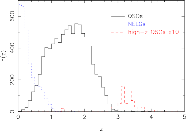
Figure 7: The redshift distribution of 2SLAQ observed sources. We plot the distribution of low redshift QSOs (solid black line), NELGs (dotted blue line) and high redshift QSOs (dashed red line). The distribution of high redshift QSOs, which are those selected via the high redshift colour cuts (Section 2.2.3), has been multiplied by a factor of 10.

The survey composition also varies as a function of magnitude; this is shown in Fig. 5. We have corrected these number counts for incompleteness in the spectroscopic coverage as a function of magnitude only (i.e. Fig. 4), and have not included incompleteness from colour selection or spectroscopy. At bright magnitudes ($g<21$) the QSOs dominate the sample, the stars are the next largest population, followed by NELGs (we’ve also included here the small number of absorption line galaxies, classified as ’gal’) and lastly, unidentified objects. At $g>21$ QSOs are still the largest single population, but the other populations become more significant. This is because of the intrinsic flattening of the QSO number counts (e.g. see R05), reduced completeness for QSOs from increased photometric errors and increased contamination from the large number of faint galaxies (and increased photometric errors). In fact, in the faintest bin the number of NELGs exceeds the number of QSOs. This is more clearly seen in Fig. 6a which shows the relative fraction of objects of each type. Our spectroscopic incompleteness (i.e. the fraction of objects with no spectroscopic identification) increases towards the faint limit of the sample. Fig. 6b shows the fraction of identification qualities as a function of $g$. The fraction of quality 1 identifications declines to 73 per cent at the faint limit of the survey. Of the remaining objects, 1/3 have quality 2 identifications and 2/3 have quality 3 identifications (the poorest). For most analyses in this paper, only quality 1 identifications are used.

The redshift distribution of the main low redshift QSO sample is shown in Fig. 7 as the solid line. The number of QSOs is relatively constant between $z\simeq 0.8$ and $2.2$, declining towards lower and higher redshift. The high redshift sample (Section 2.2.3) primarily samples the redshift range between $z\simeq 2.8$ and $4.0$, with the highest redshift QSO being J143250.16+001756.3 at $z=4.8356$. The NELGs (including some absorption line galaxies) are peaked at low redshift, with a tail of objects to $z\simeq 1$. Example 2SLAQ spectra, including a range of QSO redshifts and magnitudes as well as a NELG and a Galactic star, are shown in Fig. 8.

Figure 8: Example 2dF spectra from the 2SLAQ survey taken from observations of the e01 field in April 2005. a), b) and c) show QSOs from the main low-redshift sample, d) shows the highest redshift QSO from the high-redshift sample, e) is a typical NELG and f) shows a Galactic star. The magnitudes displayed are PSF $g$-band magnitudes (not extinction corrected), apart from d) in which we give the PSF $i$-band magnitude. The spectra are not spectrophotometrically calibrated, so the concave spectral shape is due to the instrument response.

4.2 Repeatability of identifications and redshifts

A critical test of the quality of the catalogue is to assess the reliability and repeatability of our identifications and redshifts. We can do this both internally, using repeat observations, and externally using comparisons to other catalogues. In particular, we have 2SLAQ spectra for objects which also have SDSS and 2QZ spectra available. In this external check it is worth noting that the overlap between SDSS/2QZ and 2SLAQ is only at the bright end of the sample, where identifications are inherently more reliable. Secondly, the 2QZ is only nominally an external check, as the data acquisition, reduction and analysis for 2QZ and 2SLAQ are almost identical.

We start by assessing the relative reliability of the identifications between surveys. In Table LABEL:tab:failures we list the number of objects with different quality identifications in more than one sample, compared to the number for which that identification disagrees between samples. For good quality identifications ($Q_{\rm ID}=1$) in two samples we find that 4/516 objects disagree between SDSS and 2QZ ($0.8\pm 0.4$ per cent), 4/378 between SDSS and 2SLAQ ($1.1\pm 0.5$ per cent) and 15/771 between 2QZ and 2SLAQ ($2.0\pm 0.5$ per cent). By visually examining the spectra we find that for all four SDSS-2QZ discrepancies the SDSS identification is correct. For the SDSS-2SLAQ comparison we find the SDSS identification to be correct in 3 cases and the 2SLAQ identification to be correct in 1 case. All 4 objects have the same redshift in both samples, and the disagreement is due to classification as NELG or QSO. For the 2QZ-2SLAQ comparison we found 5 cases in which the 2QZ identification was correct and 10 cases were the 2SLAQ identification was correct. Of these 10, eight were low $S/N$ objects in 2QZ wrongly classified as stars. If we compare lower quality identifications we find that, as expected, the repeatability is poorer (final three columns in Table LABEL:tab:failures).

Table 8: The fraction of objects which have different identifications (i.e. QSO vs. star etc.) in the different surveys (SDSS/2QZ/2SLAQ). 1-1 denotes a quality 1 ID for both the first and second catalogue listed in the first column; 1-2 denotes a quality 1 and a quality 2 ID for the first and second catalogues listed etc.

Surveys	$Q_{\rm ID}$	$Q_{\rm ID}$	$Q_{\rm ID}$	$Q_{\rm ID}$
	1-1	2-2	1-2	2-1
SDSS-2QZ	4/516	0/0	5/11	0/19
SDSS-2SLAQ	4/378	0/0	0/1	0/8
2QZ-2SLAQ	15/771	3/3	2/9	36/90

Table 9: The fraction of objects with the same identification which have different redshifts in the different surveys (SDSS/2QZ/2SLAQ). 11-11 denotes a quality 11 spectrum for both the first and second catalogue listed in the first column; 11-12 denotes a quality 11 and a quality 12 spectrum for the first and second catalogue listed etc.

Surveys	$Q_{\rm ID}$	$Q$	$Q$	$Q$	$Q$
	1-1	11-11	11-12	12-11	12-12
SDSS-2QZ	3/512	2/510	1/2	0/0	0/0
SDSS-2SLAQ	2/374	2/374	0/0	0/0	0/0
2QZ-2SLAQ	20/756	10/720	1/5	9/31	0/0

Next we check the external reliability of the redshift estimates. We search for objects identified in more than one sample that have the same identification (with $Q_{\rm ID}=1$) but a redshift difference of greater than $\Delta z=0.05$ (chosen to include only those objects with catastrophic failures in redshift). This resulted in 3/512 for the SDSS-2QZ comparison, 2/374 for the SDSS-2SLAQ comparison and 20/756 in the 2QZ-2SLAQ comparison. However, for a number of objects the redshift was flagged as uncertain (i.e. $Q_{\rm z}=2$). If we limit ourselves to objects with $Q=11$ (i.e. $Q_{\rm ID}=1$ and $Q_{\rm z}=1$) then the fractions are 2/510, 2/374 and 10/720 respectively (see Table LABEL:tab:failuresz). Visual assessment of the spectra for which there were discrepant redshifts showed that the surveys scored 2-1 (SDSS-2QZ), 2-0 (SDSS-2SLAQ) and 1-19 (2QZ-2SLAQ). The most common error was a confusion between Mg II and C IV, particularly when C III] was weak.

We can similarly check the reliability of our identifications and redshifts with internal checks using the repeat observations of 2SLAQ sources. A total of 3317 objects were repeated, of which 2911 had two observations, 382 had three observations, 23 had four observations and a single object had five observations. These repeats were generally made when overlapping fields were observed, and are biased towards objects which had a poor identification in one or more observation. However, there are 1672 objects with at least two observations which have both have quality 11. Of these, 1585 had identical identification and redshift ($\Delta z<0.05$) and 87 did not match. Thus the quality 11 objects are reliable at the 95 per cent level. Of the 87 that do not match, 33 have the same identification, but a different redshift (mostly QSOs, but with some NELGs). The remainder (54) have different identifications, and of these 12 have the same redshift but were identified as QSO from one spectrum and NELG in the other. This is usually due to a weak broad component combined with a stronger narrow component in the H $\beta$ line that is not identified in one spectrum (typically that with lower $S/N$).

Figure 9: The fraction of good quality identifications that are QSOs, stars and NELGs (filled squares, triangles and circles respectively) compared to the fraction of poor ($Q_{\rm ID}=2$ or 3) identifications that are QSOs, stars and NELGs (open squares, triangles and circles respectively), derived from repeat observations. Errors are only plotted for the open symbols. For the filled symbols the errors are generally the size of the symbol or smaller.

Another important question to address is the content of the unidentified objects. At the faint limit of the sample, this reaches 27 per cent (quality 2 and 3 identifications); see Fig. 6b. A first order assessment of the content of these low quality spectra can be made by comparing repeats that have one high quality ($Q_{\rm ID}=1$) and one low quality ($Q_{\rm ID}=2$ or 3) spectrum. This enables us to assess the fraction of QSOs, stars and NELGs that are contained within the unidentified objects. Fig. 9 shows the fraction of these repeats that have a good ID that is a QSO, star or NELG (open symbols). This is compared to the fractions among all the high quality objects (i.e. not just those with repeats; filled symbols). We see that at all magnitudes the QSO fraction in the identified and unidentified objects is similar. The fraction of NELGs in the unidentified objects is significantly lower than in the whole sample, while the fraction of stars is higher. This is to be expected given the ease of identifying NELGs with their strong narrow emission lines and the difficulty of identifying stars with their relatively weak absorption features. This analysis does not account for all the unidentified objects in our sample, as some are not identified even with a second observation. In the half magnitude bins from $g=20$ to $g=22.5$ used in Fig. 9, the fraction of poor spectra not identified in a second observation is 8, 11, 22, 31 and 51 per cent from bright to faint magnitudes. Therefore, for all but the faintest bin (which contains a small number of objects with high extinction and the high redshift QSO candidates), most objects are identified with a second spectrum.

Finally we assess the internal reliability of our redshift estimates. There are 1672 objects with repeats that are both quality 11. Of these 33 (2.0 per cent) have different redshifts. There are 156 repeated objects with both a quality 11 and 12 observation, of which 37 (24 per cent) have different ($\Delta z>0.05$) redshifts. This higher fraction is expected for objects with quality 2 redshift determinations.

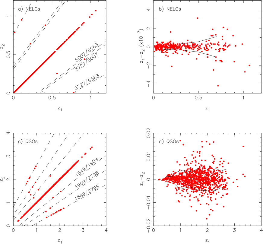
Figure 10: a) Comparison of redshifts from repeat observations of NELGs. Most lie close to the $z_{1}=z_{2}$ line, while there are a few outliers. The dashed lines show the redshift differences caused by confusing specific emission lines (rest wavelengths shown). b) Redshift difference vs. redshift for NELGs, the solid lines show the RMS scatter as a function of redshift. c) and d) are the same as a) and b) only for QSOs rather than NELGs. In all cases only quality 11 observations were considered.

We assess the accuracy of our redshift estimates by examining the scatter in redshifts for repeat observations (quality 11 only); see Fig. 10. We do this separately for NELGs and QSOs, as the NELGs with their narrow lines have a much smaller dispersion than the QSOs. Most repeat redshifts lie close to the line $z_{1}=z_{2}$. However a small number lie along lines denoting incorrect emission line identifications (dashed lines in Fig. 10). 7/385 NELGs (1.8 per cent) with repeats have discrepant redshifts due to mis-identification of emission lines. 26/1032 QSO repeats (2.5 per cent) have discrepant redshifts, of which half are due to confusion between Mg II and C IV. The scatter in redshift measurement after removing these catastrophic failures is shown in Figs. 10b and d for NELGs and QSOs respectively. The solid lines show the RMS scatter in $\Delta z=0.2$ bins (calculated for bins with greater than 10 objects). The scatter in NELG redshifts is small, $\sigma(z_{1}-z_{2})=0.00044$ ($\simeq 130$km s^-1). The scatter increases with redshift, being 0.00029 at $z=0.1$ and 0.0011 at $z=0.7$. A similar trend is seen for the QSOs, but with a larger mean scatter of $\sigma(z_{1}-z_{2})=0.0037$. We find that $\sigma(z_{1}-z_{2})=0.0014(1+z)$ gives a good description of the scatter in QSO redshifts as a function of redshift, identical to that found by Croom et al. (2005) for the 2QZ (this is not surprising given the identical spectrographic configuration and similar data quality).

5 Survey completeness

We now discuss quantitative assessments of the completeness of the 2SLAQ QSO sample. In general we can separate the completeness into four distinct types, which are a function of $g$-band magnitude, redshift $z$ (below $z$ denotes redshift rather than $z$-band magnitude) and celestial position ($\alpha,\delta$).

• Morphological completeness, $f_{\rm m}(g,z)$. This describes our effectiveness at differentiating between point and extended sources in the SDSS imaging. We include extended sources in the low redshift QSO sample.

• Photometric completeness, $f_{\rm p}(g,z)$. This attempts to take into account any QSOs which may have fallen outside our colour selection limits.

• Coverage completeness (or coverage), $f_{\rm c}(\alpha,\delta,g)$. This is the fraction of 2SLAQ sources which have spectroscopic observations.

• Spectroscopic completeness, $f_{\rm s}(\alpha,\delta,g,z)$. This is the fraction of objects which have spectra with quality 1 identifications.

5.1 Morphological completeness

As discussed by R05, we initially included in our sample objects that the SDSS photometric pipeline (PHOTO; Lupton et al 2001) classify as extended. This is because a significant number of point sources are mis-classified as extended at the faint limit of our sample ($\sim 15$ per cent; see Fig. 5 of R05) and low redshift QSOs can be genuinely extended. However, our first observing runs (March and April 2003) showed the sample contained large numbers of NELGs, of which many were extended. To reduce the contamination by NELGs, the final sample cuts were more restrictive and included morphology restrictions using the Bayesian star-galaxy classifier of Scranton et al. (2002). These are described in detail in Section 2.2. A total of 2144 objects were observed with the preliminary colour selection, of which 1021, 590, 283 and 250 were QSOs, NELGs, stars and ?? identifications, respectively. Of these sources, 284 were subsequently rejected from the final catalogue on the basis of morphology, of which 262 were NELGs, 9 QSOs, 7 stars and 6 unclassifiable. This morphological cut removed 44 per cent of the NELG contamination while only losing 0.9 per cent of the QSOs. The QSOs rejected by this cut are at low redshift, between $z=0.12$ and $0.84$, and are distributed uniformly within this interval. Thus at low redshift we do lose some QSOs due to the extended nature of their hosts. The 7 stars rejected (all with $g>20.7$) suggest that at the faint limit the Bayesian star-galaxy classifier is not perfect, so that a small number of QSOs would be lost from the sample even though their true morphology was point-like. Hence, the accuracy of the Bayesian star-galaxy classifier, together with our conservative cuts, means that the rejection of low redshift QSOs is minimal, and we will generally not correct for it in our analysis below.

As we incorporate 2QZ redshifts into the 2SLAQ catalogue, another issue to consider is that the 2QZ selection only included point-sources from APM scans of UKST photographic plates. C04 and Smith et al. (2005) discuss the morphological selection of the 2QZ in detail. There are two types of morphological incompleteness. The first is due to objects which are true point sources but which the APM software has classified at extended. From comparisons to SDSS imaging data Smith et al. (2005) show this to be a weak function of magnitude, rising from 6.4 per cent at the bright end and 8.9 per cent at the faint end. Secondly, there are objects which are truly extended (and classified as such from UKST plates), and are therefore missed by the 2QZ selection. C04 argue that this should only be a significant effect at $z<0.4$ in the 2QZ given that the typical size of stellar images on UKST plates is 2–3 arcsec. In principle, the morphological bias of 2QZ objects could impact our 2SLAQ catalogue. This is because not all 2SLAQ selected targets have been observed spectroscopically, and those with 2QZ redshifts will preferentially be point sources. The vast majority of 2SLAQ sources with 2QZ spectra have $g=19.0-21.0$; in this interval the fraction of all QSOs which are classified as extended by SDSS (SDSS TYPE = 3) was $10.3\pm 0.4$ per cent. In contrast, $7.6\pm 0.6$ per cent of 2SLAQ QSOs which have 2QZ spectra are classified as extended. Therefore, $2.7\pm 0.7$ per cent of QSOs may be missed if only targeted with 2QZ. Given the coverage completeness in the range $\sim 70-80$ per cent for the NGP (Fig. 4), the actual morphological bias introduced by the 2QZ selection will only be at the 0.5–0.8 per cent level at worst. We therefore do not account for this insignificant bias in our analysis below.

5.2 Photometric completeness

In order to determine the completeness of our sample, we construct a set of model QSO colours. In doing this we aim to trace as accurately as possible the underlying distribution, including the evolution of colour with redshift and a detailed consideration of the effects of host galaxies. These model colours are then passed through our selection algorithm to estimate the fraction of objects selected. We use a modified version of the technique described by R05 (and Fan 1999), but unlike them, we also incorporate the impact of host galaxies.

5.2.1 Simulating QSO colours

We start by generating a set of QSO-only spectral energy distributions (SEDs) (i.e. not including host galaxy contributions) which are well matched to the colours of bright ($i<18$) SDSS QSOs taken from the DR3 catalogue [Schneider et al. 2005]. These are similar to those generated by various other authors (e.g. Fan 1999; Richards 2006). The underlying continuum is assumed to be a power law in frequency, $\nu$, of the form $f_{\nu}\propto\nu^{\alpha_{\nu}}$ (equivalent to a power law in wavelength of $f_{\lambda}\propto\lambda^{-[\alpha_{\nu}+2]}$). The power law index, $\alpha_{\nu}$ is normally distributed with a mean $\alpha_{\nu}=-0.3$ and a standard deviation of 0.3. A mean of $\alpha_{\nu}=-0.3$ is slightly bluer than that assumed by some other authors (e.g. Richards et al. (2006) used $<\alpha_{\nu}>=-0.5$). We find that the bluer $\alpha_{\nu}=-0.3$, provides a better match to the observed colours of bright QSOs. This may be because the measured redder slopes already include some contribution from their host galaxy.

We then include an emission line component using the SDSS QSO composite [Vanden Berk et al. 2001]. We divided the composite spectrum by a fit to the continuum at $\lambda<5000$Å then subtract a second power law red-ward of this limit. The composite is seen to have a redder spectrum at $\lambda>5000$Å; probably due to contamination of low redshift QSOs by a host galaxy contribution, which we wish to remove before creating our emission line spectrum. Hence we subtract the continuum red-ward of this limit rather than dividing by it. All emission lines are assumed to have the same relative equivalent width (EW), but the emission line spectrum is scaled by a factor that has a log-normal distribution with a mean of 1 and $\sigma=0.48$, consistent with the measurements made of the EW distribution of 2QZ QSOs by Londish (2003). We also make a correction to the flux around the Lyman-$\alpha$ line to account for absorption already present in the composite spectrum. To match the $u-g$ colours of QSOs at $z\sim 1.5-2.2$ we boost the flux at $\lambda=1180-1290$Å by a factor of 1.2. We add a Balmer continuum (BC) component to the QSO spectrum of the form given by Eq. 6 in Grandi (1982). We use a temperature of 12000K and the relative normalization of the BC component that is 0.05 of the underlying continuum at 3000Å, which we find matches the observed colours of bright QSOs. This is somewhat lower than the 0.1 fraction used by Maddox & Hewett (2006) in their generation of simulated QSO spectra. We suspect that this difference is due to the fact that the emission line spectrum we use effectively contains some fraction of the BC component as well.

Table 10: Parameters of the assumed distribution of Lyman-$\alpha$ forest, Lyman-limit and damped absorbers. The evolution of the absorbers is modelled by a power law of the form $N(z)=N_{0}(1+z)^{\gamma}$ and the H I column distribution is proportional to $N_{\rm H}^{-\beta}$. $b$ is the Doppler width of the Voigt profile. Note that these parameters are the same as those given by Fan (1999) with the exception of $N_{0}$ for the Lyman-$\alpha$ forest (Fan et al. used $N_{0}=50$).

Absorption type	$\log(N_{\rm H})$	$N_{0}$	$\gamma$	$\beta$	$b$
	(cm-2)				(km s-1)
Lyman-$\alpha$ forest	13.0–17.3	20.0	2.3	1.41	30
Lyman-limit	17.3–20.5	0.27	1.55	1.25	70
Damped Lyman-$\alpha$	20.5–22.0	0.04	1.3	1.48	70

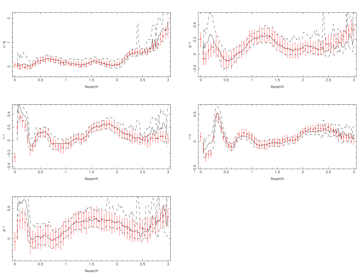
Figure 11: The median simulated QSO colours not including host galaxy contributions (filled circles) compared to QSOs with $i<18$ from the SDSS DR3 QSO catalogue (Schneider et al 2005; solid line). The error bars on the points show the 68 percentile range for the simulated colours (equivalent to $1\sigma$ Gaussian errors) and can be compared to the same range shown for the SDSS DR3 QSOs (dashed lines). The simulated colours match the observed colours well at redshift $z>0.25$. Below this redshift, even the relatively bright QSOs from DR3 are affected by some host galaxy contamination.

Absorption blue-wards of Lyman-$\alpha$ is added to the spectrum following the recipe of Fan (1999) with some minor modifications. We calculate the contributions to the opacity for the first 10 transitions and use the accurate approximation of Tepper García (2006) to calculate Voigt profiles (although note that they have an error in the equation in footnote 4 of their paper, and $Q\equiv 1.5/x^{2}$ rather than $Q\equiv 1.5x^{2}$). For each absorber the Lyman limit absorption was calculated using the prescription of Kennefick et al. (1995). The forest, Lyman-limit and damped absorbers are each distributed according to the values listed in Table LABEL:tab:lyman, which follows closely the values listed by Fan (1999) except for the value of $N_{0}$ for the Lyman-$\alpha$ forest. We find a better match to the QSO colours with a lower value than Fan (1999).

Next, asinh magnitudes in the SDSS bands are calculated from the QSO SEDs, including the small corrections to transform from true AB to the SDSS system ($u_{\rm AB}=u_{\rm SDSS}+0.04$ and $z_{\rm AB}=z_{\rm SDSS}+0.02$) [Abazajian et al. 2004].

Finally, we add a Gaussian random error with a $\sigma$ drawn from the SDSS PSF magnitude errors at the simulated magnitudes. This error was combined in quadrature with the uncertainties in the photometric calibration (0.03 in $u$ and $z$, and 0.02 in $g$, $r$ and $i$). The colour redshift relations for these (QSO only) simulations are shown in Fig. 11. In this plot we show the four usual colours: $u-g$, $g-r$, $r-i$ and $i-z$ as a function of redshift. We also show $g-i$ which, although not independent of the first four colours, is one of the primary colours used in 2SLAQ selection. We compare these relations to those derived from SDSS QSOs from the DR3 QSO catalogue [Schneider et al. 2005] with $i<18$. This brighter magnitude was chosen to reduce the effect of host galaxy contamination on the observed colours at low redshift. The median simulation colours accurately track the observed medians over almost the entire range sampled. At $z<0.25$ the simulated colours are consistently bluer than the observed colours by up to $\sim 0.2$ mag. This we ascribe to the effect of host galaxy contamination in these low redshift sources. At $z>2.5$ there is some evidence that the simulated $r$-band magnitudes are $\sim 0.1-0.15$ mag too bright (seen in the $g-r$ and $r-i$ vs redshift plots). This could plausibly be due to the models having too much C IV flux at this redshift. Fig. 11 also shows the 68 percentile range for the simulations (errorbars on points) and the data (dashed lines). These are also in excellent agreement for all but the lowest redshift intervals ($z<0.25$). In summary, over the redshift range for which the 2SLAQ survey has high completeness ($0.4<z<2.6$; see below), the model QSO colours are an excellent match to the observed colours of bright QSOs.

5.2.2 Simulating host galaxy colours

Now that we have a reliable method for simulating QSO spectra, we must consider the impact of the host galaxy on the final observed colours of 2SLAQ objects. The 2SLAQ selection is based on SDSS PSF photometry, so host galaxy contributions are to some extent minimized, but at the faint flux limits we reach these PSF magnitudes still contain significant host galaxy contributions (e.g. Schneider et al. 2003). We start by considering the observed relation between $L_{\rm QSO}$ and $L_{\rm gal}$ from the low redshift host galaxy analysis of Schade, Boyle & Letawsky (2000). Taking this data and fitting a relation

$$M_{\rm gal}=A+BM_{\rm QSO}$$ (42)

to all objects with point source detections in the $B$-band brighter than $M_{\rm B}(AB)=-16$ we obtain $A=-17.1\pm 1.1$ and $B=0.21\pm 0.05$ with a scatter, $\sigma_{\rm qg}$=0.7 in $M_{\rm gal}$. If we instead assume no correlation between $M_{\rm gal}$ and $M_{\rm QSO}$, we find the mean $M_{\rm gal}(AB)$ is $-21.3$ with an rms scatter of 0.8. Within the luminosity range that Schade et al. probe, the $M_{\rm gal}-M_{\rm QSO}$ correlation is significant, but if brighter AGN are added to the sample, the relation appears to flatten (see Fig. 13c of Schade et al.). With this in mind, below we will investigate whether we can constrain the slope of the relation by comparing our simulations and 2SLAQ colours.

Our approach is to constrain as many parameters of the host galaxy SED as possible from independent observations and then use the colour distribution of the 2SLAQ QSOs to adjust the other parameters. In particular, we need to ensure that when we apply the colour selection criteria to our simulated QSOs that we obtain the same colour distribution as for the real data. This is a necessary, but not sufficient, requirement to demonstrate that our simulations accurately model the colours of the underlying population.

Broad-band colours alone, especially when combined with a QSO SED, are not adequate to fully constrain the host galaxy SEDs. We therefore consider a number of possible star-formation scenarios and model SEDs using the Bruzual & Charlot (2003) population synthesis code. We assume a solar metallicity and Chabrier (2003) initial mass function (IMF) for all models, on the basis that high redshift QSO metallicities are typically found to be high (Dietrich et al. 2003; Kurk et al. 2007), and that with only a small number of broad-band colours we cannot hope to separate out the effects of any metallicity or IMF variation.

We first consider two burst models, either a single instantaneous burst (SIB) or a single long burst of length $\tau=1$Gyr (SLB) which occurs at high redshift ($z=10$). We then only allow passive evolution of the stellar population with redshift. In such a model, the normalization (A) in equation 42 is made relative to the expected galaxy colours at $z=0$.

The second set of models we test are those with a fixed age, based on the argument that QSOs are largely formed in galaxy mergers (e.g. Hopkins et al. 2006), which will also trigger star formation. In this scenario the dominant stellar population in QSO host galaxies would have similar ages, consistent with the time since the merger event. In this scenario we test three different star formation models, the SIB, the SLB and an exponential declining (ED) star formation rate with an e-folding timescale of 1Gyr. We also test these for a range of ages from 0.5 to 5Gyr.

We ran a suite of simulations for each of these models. For each model we fit for the best value of $A$ in Eq. 42 above, while keeping the other parameters constant. This accounts for the change in zero-point due to the differing host SEDs, as well as any host flux missed due to our use of PSF magnitudes. We then test the simulated colours against the 2SLAQ QSO sample to first confirm that they can reproduce the observed colours. Once we have ascertained that a given model is a reasonable description of 2SLAQ colours, we then generate completeness estimates as a function of redshift and $g-$band magnitude for all valid simulation parameters. These results show the likely range of completeness corrections.

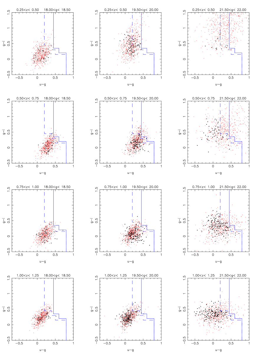
Figure 12: A comparison of 2SLAQ (black points) and simulated (red points) $u-g$ and $g-i$ colours in the redshift intervals $0.25<z<0.50$, $0.50<z<0.75$, $0.75<z<1.00$ and $1.00<z<1.25$ (top to bottom). We compare these distributions as a function of $g$-band magnitude in $\Delta g=0.5$ mag bins with $18.0<g<18.5$, $19.5<g<20.0$ and $21.5<g<22.0$ (left to right). The blue lines indicate the QSO selection limits at $g<21.15$ (solid line) and $g>21.15$ (dashed line). Both the data and simulated points show a reddening of the $g-i$ colour and increased scatter towards fainter magnitudes. The simulated points are a realization of model 2 from Table LABEL:tab:colsims, which provides one of the better matches to our data.

Table 11: The parameters and fit results for the different simulation parameters used to test 2SLAQ colour completeness. The simulation parameters include the SED model; either single instantaneous burst (SIB), single long burst (SLB) or exponential decline (ED). Also listed are the form of evolution and the input slope ($B$) and scatter ($\sigma_{\rm qg}$) in Eq. 42. The results of the fit are the best value of $A$ and $\chi^{2}$. The number of degrees-of-freedom is $\nu\simeq 68$ in each case. In two cases, both with fixed ages of 0.5 Gyr, the fit did not converge, and no best fit value is given.

#	SED	Evolution	B	$\sigma_{\rm qg}$	A	$\chi^{2}$
1	SIB	passive, $z_{\rm form}=10$	0.2	0.7	$-15.53\pm 0.03$	423
2	SLB	passive, $z_{\rm form}=10$	0.2	0.7	$-15.51\pm 0.03$	412
3	ED	passive, $z_{\rm form}=10$	0.2	0.7	$-15.44\pm 0.03$	390
4	SLB	passive, $z_{\rm form}=10$	0.0	0.8	$-19.99\pm 0.03$	326
5	SLB	passive, $z_{\rm form}=10$	0.4	0.7	$-11.05\pm 0.03$	590
6	SIB	fixed age 0.5Gyr	0.2	0.7	$-16.68\pm 0.03$	1293
7	SIB	fixed age 1.0Gyr	0.2	0.7	$-16.45\pm 0.03$	630
8	SIB	fixed age 3.0Gyr	0.2	0.7	$-16.23\pm 0.03$	485
9	SIB	fixed age 5.0Gyr	0.2	0.7	$-16.20\pm 0.03$	490
10	SLB	fixed age 0.5Gyr	0.2	0.7	–	–
11	SLB	fixed age 1.0Gyr	0.2	0.7	$-17.04\pm 0.03$	2373
12	SLB	fixed age 3.0Gyr	0.2	0.7	$-16.27\pm 0.03$	470
13	SLB	fixed age 5.0Gyr	0.2	0.7	$-16.21\pm 0.03$	506
14	ED	fixed age 0.5Gyr	0.2	0.7	–	–
15	ED	fixed age 1.0Gyr	0.2	0.7	$-16.54\pm 0.04$	3027
16	ED	fixed age 3.0Gyr	0.2	0.7	$-16.65\pm 0.03$	668
17	ED	fixed age 5.0Gyr	0.2	0.7	$-16.33\pm 0.03$	474

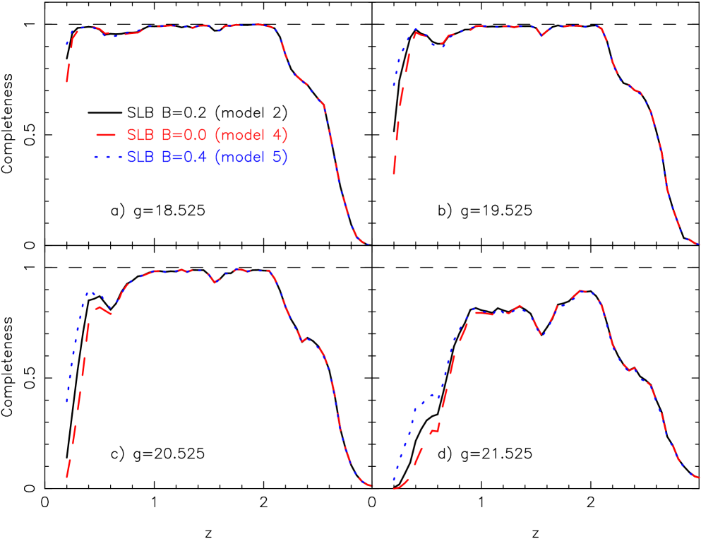
Figure 13: A comparison of photometric completeness as a function of redshift for 4 different apparent magnitude slices with mean $g$-band mag a) $g=18.525$, b) $g=19.525$, c) $g=20.525$ and d) $g=21.525$. We compare models with different values of $B$ (defined in Eq. 42), $B=0.0$ (dashed red line), $B=0.2$ (solid black line), $B=0.4$ (dotted blue line) which are models 4, 2 and 5 respectively in Table LABEL:tab:colsims. At bright magnitudes and/or high redshift all three models agree very well, while at faint magnitudes the models diverge below $z\sim 0.5$.

Table LABEL:tab:colsims contains the parameters for the various host galaxy models used in the above tests. An example of the colour distributions as a function of $g$ and redshift is shown in Fig. 12, which compares simulated colours for model 2 and observed 2SLAQ colours. To test each model we sample the redshift distribution from $z=0.1$ to 1.5 and total magnitude (nucleus + host) distribution from $g=18$ to 22, binning with $\Delta z=0.02$ and $\Delta g=0.1$. In each of these bins we generate 10 model QSO+host spectra, and then compare the derived $g-i$ colours to those from the 2SLAQ sample in order to obtain the best fit value of $A$ from Eq. 42 above. The best fit values and the resulting $\chi^{2}$ are listed in table LABEL:tab:colsims. The $g-i$ colour comparison was made with the median colours in bins of $\Delta z=0.25$ and $\Delta g=0.1$. The errors on these median values were taken as the 68 percent inter-quartile value. Only bins with 5 or more observed and simulated points were considered. The number of degrees of freedom was $\nu\simeq 68$ in each case, varying slightly due to our constraint of requiring at least 5 points in each bin. It can be seen that all the $\chi^{2}$ values are considerably larger than $\nu$, indicating that in detail our relatively simple model does not perfectly trace the distribution of QSO+host colours. We note here that we are not aiming to model the host colours in great detail, but to obtain a description of them that is sufficiently accurate to enable a reasonable estimate of completeness.

For a model with passive evolution and an early redshift of formation ($z_{\rm form}=10$) there is little difference between the models; largely because at the redshift in question, all the models SEDs are dominated by older stars. When we change the slope of the $M_{\rm gal}-M_{\rm QSO}$ relation (Eq. 42), a flatter slope is preferred according to our $\chi^{2}$ statistic. This is because a flatter slope in Eq. 42 allows the relation between $g-i$ and $g$ to be steeper. However, we note that if we push the slope to be even flatter (i.e. $B\leq 0$), then although we obtain a relatively good fit with the test described above, the simulated objects at low $z$ and faint $g$ are too red. This discrepancy does not show up in the above test because of the relatively low number of 2SLAQ objects in these bins.

Considering the models with fixed age SEDs (numbers 6–17 in Table LABEL:tab:colsims), it is clear that models with young SEDs are very much worse fits than older SEDs. The $\chi^{2}$ values increase substantially for the SIB and SLB models with ages $<3$Gyr. For the ED model, only the 5Gyr population gives as good a fit as the SIB and SLB models. The data are more consistent with an older age stellar population in the host galaxies because of the red colours of faint 2SLAQ objects in $g-i$. This can be seen in Fig 12, which shows the reddening of $\sim 0.5$ mag in $g-i$ from $g=18.0$ to 22.0, in the redshift interval $0.50<z<0.75$. A significant young and blue ($<1$Gyr) stellar population is inconsistent with the observed trend, as reflected in in the poorer $\chi^{2}$ fits in Table LABEL:tab:colsims. This could provide challenges for models of QSO formation which rely on mergers to trigger QSO activity and star formation [Hopkins et al. 2006], as it implies that the dominant stellar population is relatively old. However, given that the objects in question are at low redshift and low luminosity, it could be that major mergers do not play such a significant role for this faint population [Hopkins & Hernquist 2006]. Indeed, various observations of more luminous QSO have found evidence that the hosts are bluer than typical galaxies, with relatively young stellar populations (e.g. Kirhakos et al. 1999; Zakamska et al. 2006). At low redshift ($z<0.3$) Kauffman et al. (2003) show that the stellar populations in the host galaxies of type II AGN are similar to non-active early type galaxies, although at high luminosity the stellar population becomes younger (as measured by the $D_{\rm n}(4000)$ index). Vanden Berk et al. (2006) find that hosts of SDSS quasars at $z<0.75$ span a wide range of spectral types, but at low host (and nuclear) luminosity the typical colours are similar to non-active early types. Our estimates of host galaxies properties seem broadly consistent with this work.

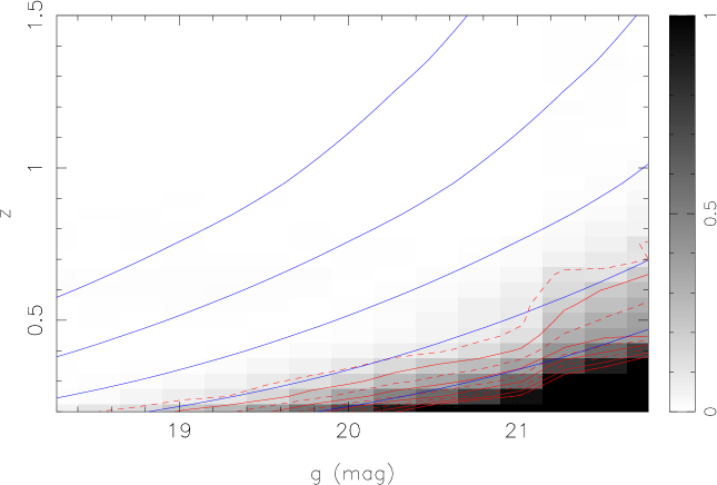
Figure 14: The fractional difference between completeness estimates assuming host galaxy models 2, 4 and 5. We plot $0.5(C_{4}-C_{5})/C_{2}$ where $C_{4}$ is the completeness in model 4 etc. The contours are at 0.1 intervals (0.1, 0.3… dashed red lines; 0.2, 0.4… solid red lines), and the same data are also plotted as a grey-scale. The solid blue lines denote lines of constant absolute magnitude from $M_{\rm g}=-24$ (top) to $M_{\rm g}=-20$ (bottom) in 1.0 mag intervals. At $M_{\rm g}=-21$ the uncertainty in the completeness is always less than 20 per cent. Note the more limited redshift range compared to Fig. 15 below.

The final step is to compare the completeness estimates from the different models in order to determine the uncertainty in our completeness corrections. We simulate the redshift range $0.1<z<3.0$ and use $18<g<22$. We use the bins $\Delta z=0.02$ and $\Delta g=0.1$ and increase the number of simulated objects to 200 per bin, so that our completeness estimates are not limited by shot-noise. We find that the largest variation in estimated completeness from within our suite of models is due to the variation in the parameter $B$ in Eq. 42. In Fig. 13 we plot models 2, 4 and 5 from Table LABEL:tab:colsims for four different $g$-band magnitude slices. It is only at faint magnitudes and redshifts less than $\sim 0.5$ that the completeness depends on the model. To quantify this further, Fig. 14 plots the mean fractional difference in the models, i.e. $0.5*(C_{4}-C_{5})/C_{2}$, where $C_{2}$ is the completeness in model 2 etc. We overlay contours of constant absolute $g$-band magnitude (blue lines) from $M_{\rm g}=-24$ (top) to $-20$ (bottom) (using the Cristiani & Vio 1990 K-correction). Brighter than $M_{\rm g}\simeq-21$ the uncertainty on the completeness estimate is less than 20 per cent and by $M_{\rm g}\simeq-21.5$ this uncertainty is less than 5 per cent.

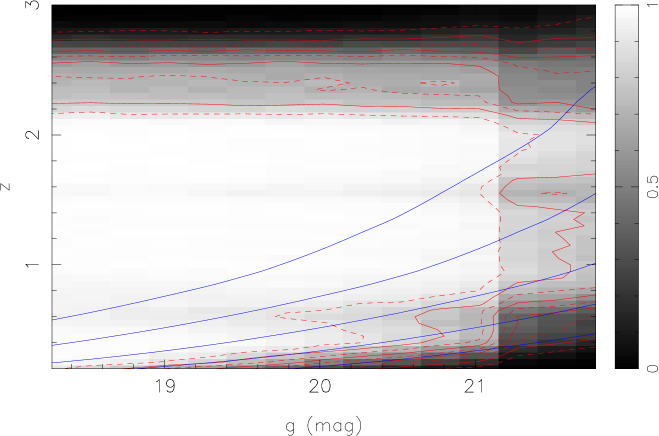
Figure 15: The final photometric completeness map for the 2SLAQ sample as a function of $g$ and $z$ assuming model 2. The contours are at 0.1 intervals (0.1, 0.3… dashed red lines; 0.2, 0.4… solid red lines), and the same data are also plotted as a grey-scale. The solid blue lines denote lines of constant absolute magnitude from $M_{\rm g}=-24$ (top) to $M_{\rm g}=-20$ (bottom) in 1.0 mag intervals.

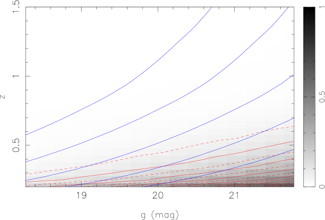
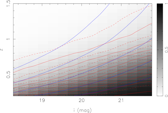
Figure 16: Top: the fractional contribution of the host galaxy to the total $g$-band PSF flux of 2SLAQ QSOs as a function of $g$ and $z$ (assuming model 2 from Table LABEL:tab:colsims). The contours are at 0.05 intervals (0.05, 0.15… dashed red lines; 0.1, 0.2… solid red lines), and the data are also plotted as a grey-scale. The solid blue lines denote lines of constant absolute magnitude from $M_{\rm g}=-24$ (top) to $M_{\rm g}=-20$ (bottom) in 1.0 mag intervals. Bottom: same as above, but showing the fractional contribution of the host galaxy to the total $i$-band PSF flux as a function of redshift and $i$-band flux. At low redshift and faint $i$-band flux, these $i$-band host contributions are extrapolated from the comparison to the 2SLAQ data. This is because the combined QSO+host colours are relatively red, $g-i\sim 1$, so that a source with $i\simeq 22$ will be $\sim 1$ mag fainter than the 2SLAQ $g$-band limit.

Table 12: The 2SLAQ colour completeness array. The completeness is given as a function of redshift, $z$, and $g$-band magnitude. We also list the host galaxy contribution as a magnitude difference, $\Delta$host in both the $g$ and $i$ bands. The first ten rows are given here. The full table is available in the electronic version of the journal.

$z$	Mag.	Completeness	$\Delta$host	$\Delta$host
	$g$/$i$		$g$ (mag)	$i$ (mag)
0.200	18.275	0.92	0.19	0.81
0.200	18.525	0.85	0.23	0.99
0.200	18.775	0.79	0.27	1.11
0.200	19.025	0.69	0.31	1.26
0.200	19.275	0.62	0.36	1.41
0.200	19.525	0.52	0.40	1.55
0.200	19.775	0.40	0.46	1.73
0.200	20.025	0.31	0.53	1.91
0.200	20.275	0.23	0.60	2.10
0.200	20.525	0.14	0.68	2.29

Based on this we adopt model 2 for our final colour completeness. This provides a reasonable match to the observed 2SLAQ QSO colours as well as being mid-way between the models with the largest variations (i.e. models 4 and 5). The completeness array for this model is shown in Fig. 15. The step at $g=21.15$, where we change our colour selection limits, is clearly visible. In contrast to our previous estimates of the completeness of 2SLAQ selection (see R05), the completeness derived here declines much more at faint magnitudes and low redshift. Table LABEL:tab:colcomp contains the colour completeness array as a function of $z$ and $g$. The full table is available in the electronic version of the journal.

5.2.3 Correcting for host galaxy flux

Our detailed simulations enable a relatively straightforward mechanism to correct the photometry of the 2SLAQ QSOs for the contribution of their host galaxy. The photometry used to select targets and calculate luminosities was based on SDSS PSF magnitudes, so this should limit the contribution of the host to some extent, but up to $z\simeq 1$ there is some contribution from the host in the PSF magnitudes. For each simulated source we calculate the total PSF magnitude ($m_{\rm tot}$, QSO+host) and the difference between total and the QSO, $m_{\rm QSO}-m_{\rm tot}$. We can then derive the mean correction from total to nuclear magnitude in the same $g$-band and redshift intervals used to make the completeness correction array. Fig. 16 shows the fractional host contribution to the PSF flux in the $g$ (top) and $i$ (bottom) bands. In the $g$-band, which forms the flux limit of the 2SLAQ sample, the host contribution is less than 20 per cent at $z>0.4$, even for the faintest sources. However, it is not until $z\sim 0.9$ that the contribution falls below 20 per cent in the $i$-band. These corrections can be applied to determine nuclear fluxes for 2SLAQ sources. The host galaxy contributions as a function of redshift and $g$ and $i$ band magnitude are listed in Table LABEL:tab:colcomp.

5.3 Coverage completeness

The coverage completeness in the 2SLAQ survey is a function of both celestial position and $g$-band magnitude. The global coverage as a function of $g$ is shown in Fig. 4. The step at $g=20.5$ is due to the prioritization of faint QSOs, while the increasing completeness from $g=20.5$ towards bright magnitudes is due to our inclusion of observations from the 2QZ and SDSS surveys. This global coverage completeness is all that is required for analyses such as luminosity function calculations.

The angular dependence on the sky of the coverage is a fixed value for each sector made up by the intersection of overlapping 2SLAQ fields. However, the geometry of these fields is more complex than in the case of 2QZ, as we must account for the triangular exclusion regions around the edge of each field (Fig. 2). Once these areas are accounted for we are able to construct a completeness mask with $1\times 1$ arcmin pixels which describes the angular coverage of the survey.

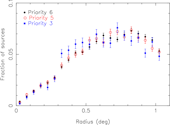
Figure 17: The fraction of 2SLAQ objects targetted spectroscopically as a function of radius from the 2dF field centre in bins of $\Delta r=0.05^{\circ}$. We plot the radial distribution for the priority 6 (black filled circles), 5 (red open circles) and 3 (blue filled squares).

A second complication is that because of the biases in the CONFIGURE software [see Section 3.2 above and Mizarksi et al. (2006)] it is possible that targets at different priorities could be distributed differently within a 2dF field. We test this by comparing the spatial distribution of our highest priority QSOs (priority 6; see Table 3) and the priority 5 and 3 QSOs (there are too few priority 4 QSOs to make a meaningful comparison). We carry out two tests. The first is to bin the observed objects as a function of radius from their field centre, with $\Delta r=0.05^{\circ}$ (see Fig. 17). A $\chi^{2}$ test between priority 6 and 5 objects gives $\chi^{2}/\nu=24.17/21$ which is only inconsistent at the 28 per cent level. By contrast comparing priority 6 and 3 we find $\chi^{2}/\nu=54.80/21$, which infers a probability of being drawn from the same population of $7.56\times 10^{-5}$. We also compare the distributions using a 2D KS test, where the two dimensions correspond to the angular coordinates ($\alpha$, $\delta$) of the QSOs on the sky. For the priority 6/5 comparison this gives $D_{\rm KS}=0.0224$ and $P(>D_{\rm KS})=0.11$, while for the priority 6/3 comparison we find $D_{\rm KS}=0.103$ and $P(>D_{\rm KS})=1.013\times 10^{-15}$. Thus we conclude that there is no statistically significant difference in the spatial distribution of priority 5 and 6 objects, but that the priority 3 sources (bright, $g<20.5$ QSOs) do have a significantly different spatial distribution. These objects should then not be used for analyses in which spatial distribution is important (e.g. clustering measurements).

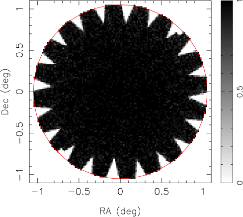
Figure 18: The 2SLAQ QSO coverage mask for a single 2dF field, determined by averaging over many configurations of random simulations. The greyscale gives the probability of being able to configure an object. The mask is defined in $1\times 1$ arcmin pixels, and the plotted (red) circle defines the $1.05^{\circ}$ radius field-of-view. The inaccessible wedges around the edge of the field are clearly visible. The small holes near the bottom left ($\alpha=\delta=-0.7^{\circ}$) and top right ($\alpha=\delta=+0.7^{\circ}$) of the field are due to two retaining screws in the field plate, over which fibres cannot be placed.

Figure 19: The 2SLAQ coverage mask, defined as the fraction of priority 5 and 6 targets (QSO candidates with $g>20.5$) that have been spectroscopically observed. The grey-scale extends from 0.0 (white) to 1.0 (black). The solid red lines mark the extent of the input catalogue regions. a) The a and b regions in the NGP; b) the c, d and e regions in the NGP, c/d) the single s region in the SGP. While there is almost complete coverage in the NGP regions (apart from the a region at $\alpha=123$ to $144$ deg), large parts of the SGP region remain unobserved.

Figure 20: The 2SLAQ spectroscopic completeness mask, defined as the fraction of observed priority 5 and 6 objects which have high quality identifications (ID quality = 1). The grey-scale extends from 0.0 (white) to 1.0 (black). The regions plotted are the same as in Fig. 19.

We derive the average mask for a single 2dF pointing, taking into account the inaccessible wedges near the edge of the field. This is done by running the CONFIGURE software in batch mode for 1000 realizations. The resulting single field mask is shown in Fig. 18. This is then converted to a binary mask (i.e. 1 if observable, or 0 if not) to define the boundaries for each field. With the geometry of each field defined, we determine a set of unique sectors formed from the overlap of all the observed 2SLAQ fields. Within each sector we then derive the fraction of priority 5 and 6 objects observed. This is then sampled onto $1\times 1$ arcmin pixels. The resulting coverage masks for the NGP and SGP regions are shown in Fig. 19. As this mask is for the priority 5 and 6 objects only, it has no magnitude dependence and it is a function of angular celestial position only, i.e. $f_{\rm c}(\alpha,\delta)$. Another issue to consider when studying the spatial distribution of the 2SLAQ QSOs is that the 2SLAQ LRGs were given higher priority. Thus the regions within $\simeq 30$ arcsec of the LRGs (Cannon et al. 2006) represent regions of sky that were not surveyed, and these need to be included in the coverage mask. This has been done for the QSO clustering analysis presented by da Angela et al. (2008). The masks presented in this current work are not corrected for the LRG distribution.

5.4 Spectroscopic completeness

We specify the spectroscopic completeness as the ratio $N_{1}/N_{\rm obs}$, where $N_{1}$ is the number of quality 1 IDs and $N_{\rm obs}$ is the number of targets observed. The global spectroscopic completeness is shown in Fig. 6b as a function of $g$-band mag only. In general this is a function of angular position (due to varying observing conditions etc.) and redshift (due to different emission lines moving in and out of the observed spectral range) as well as $g$. We make the assumption that the fraction of QSOs among the unidentified objects is the same as that within the sample of high quality identifications. We saw that this is reasonable from our analysis of repeat observations in Section 4.2. Below we follow C04 to generalize the spectroscopic completeness estimate to be a function of celestial position ($\alpha,\delta$), $g$-band magnitude and redshift.

5.4.1 Position-dependent spectroscopic completeness

We can generate a position dependent spectroscopic completeness mask, $f_{\rm s}(\alpha,\delta)$, similar to the coverage mask presented above. The mean spectroscopic completeness per sector is shown in Fig. 20. Because the observations were extended during poor observing conditions, the spectroscopic completeness is relatively uniform.

5.4.2 Magnitude-dependent spectroscopic completeness

Figure 21: The 2SLAQ spectroscopic completeness as a function of $g$-band magnitude for sectors with different mean completeness values, $\langle f_{\rm s}(\alpha,\delta)\rangle$. In each case the best fit magnitude-dependent completeness model (Eq. 43) is shown (solid line).

Figure 22: The magnitude dependent spectroscopic completeness parameter, $\mu$, as a function of mean sector spectroscopic completeness, $\langle f_{\rm s}(\alpha,\delta)\rangle$ (filled circles). The solid line shows the best fit of Eq. 44 to this data.

Some analyses, e.g. luminosity dependent clustering measurements, will require that the magnitude dependence of the completeness variations are accurately mapped over the 2SLAQ regions. Following C04, we determine the magnitude dependent spectroscopic completeness, $f_{\rm s}(g)$, within sectors of varying completeness. This is plotted in Fig. 21. For fields with high average completeness, there is very little magnitude dependence, but the magnitude dependence becomes stronger as the average completeness declines. We parameterize the magnitude dependence of completeness by the function

$$f_{\rm s}(g)=1-\exp(g-\mu),$$ (43)

where $\mu$ is a parameter fit in each magnitude bin. The best fits of this function for each average completeness interval are plotted in Fig. 21. The $\mu$ parameter varies smoothly with average completeness (see Fig. 22) and can be well described by

$$\mu=A+B\ln[1-\langle f_{\rm s}(\alpha,\delta)\rangle],$$ (44)

where $A=21.47\pm 0.11$ and $B=-0.891\pm 0.070$. The magnitude dependence of $f_{\rm s}$ in a particular sector is then described by

$$f_{\rm s}(g)=1-\frac{\exp(g-A)}{[1-f_{\rm s}(\alpha,\delta)]^{B}}.$$ (45)

This can be combined with $f_{\rm s}(\alpha,\delta)$ to give

$$f_{\rm s}(\alpha,\delta,g)=\frac{N_{\rm obs}(\alpha,\delta)}{N_{\rm est}(\alpha,\delta)}f_{\rm s}(\alpha,\delta)f_{\rm s}(g),$$ (46)

where the value $N_{\rm est}(\alpha,\delta)$ is the estimated number of quality 1 IDs given the function $f_{\rm s}(g)$ in a particular sector. This is given by

$$N_{\rm est}(\alpha,\delta)=\sum^{N_{\rm obs}(\alpha,\delta)}_{i=1}f_{\rm s}(g).$$ (47)

The angular masks containing the values of $f_{\rm s}(\alpha,\delta)$ and $N_{\rm obs}(\alpha,\delta)/N_{\rm est}(\alpha,\delta)$ are supplied as part of the 2SLAQ catalogue release.

For analyses which do not require spatial information (e.g. the luminosity function of QSOs), a global average best fit $\mu$ value can be used. For the priority 5 and 6 sample discussed here we find a global best fit $\mu=23.21\pm 0.03$. The average completeness of the sample is 85.4 per cent, which would imply $\mu=23.18$ using the best fit values of $A$ and $B$ above, in good agreement with the directly fitted value.

5.4.3 Redshift-dependent spectroscopic completeness

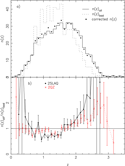
Figure 23: The redshift dependence of spectroscopic completeness in the 2SLAQ survey. a) The observed distribution of all quality 11 2SLAQ QSOs, $n(z)_{\rm all}$ (solid line), compared to the redshift distribution of objects with low-quality identifications which also obtained high-quality QSO redshifts, $n(z)_{\rm bad}$ (dotted line). $n(z)_{\rm all}$ has been renormalized to match $n(z)_{\rm bad}$. Also plotted is the corrected $n(z)$ assuming that unidentified objects are distributed as $n(z)_{\rm bad}$. b) The ratio of the normalized $n(z)_{\rm all}$ to $n(z)_{\rm bad}$ with Poisson error bars (connected filled circles) As a comparison, the same quantity derived from the 2QZ sample is also shown (red crosses).

We follow a procedure similar to that employed by the 2QZ to determine if there are any spectroscopic completeness variations as a function of redshift. To do this we use the 512 QSOs with good quality (11) IDs, that also have repeat observations of lower quality (22 or worse). We can use these repeated observations to examine the redshift distribution of unidentified objects. In Fig. 23a we plot the redshift distribution of all quality 11 QSOs observed as part of 2SLAQ (solid line), $n(z)_{\rm all}$, compared to the redshift distribution of repeated objects that had at least one bad ID as well as a good ID (dotted line), $n(z)_{\rm bad}$. The fraction of bad IDs is higher in the redshift range $z\simeq 0.5-1.6$, probably due to the changing visibility of strong emission lines as a function of redshift. In particular, the C IV emission line becomes visible in the spectra at $z\sim 1.5$ making identifications significantly easier above this redshift. The ratio of $n(z)_{\rm all}$ to $n(z)_{\rm bad}$ is shown in Fig. 23b (filled circles). If we then add in the 13.1 per cent of objects without good quality IDs in the 2SLAQ catalogue (assuming they have the same redshift distribution as $n(z)_{\rm bad}$), we get the redshift distribution given by the filled points in Fig. 23a. Thus, even though the redshift distribution of unidentified objects is quite different from the rest of the sample, the small incompleteness means that the overall $n(z)$ is changed only slightly. As a comparison we also plot the ratio of $n(z)_{\rm all}$ to $n(z)_{\rm bad}$ derived from the 2QZ (C04) (red crosses in 23b). The 2QZ and 2SLAQ samples show exactly the same trends, although the amplitude of the variations is somewhat higher for the 2SLAQ sample. This could be due to the Baldwin (1977) effect, which causes emission lines to be stronger in lower luminosity QSOs.

Table 13: Derived values for $R(z)\equiv n(z)_{\rm all}/n(z)_{\rm bad}$ (and errors, $\sigma_{R(z)}$) that can be used to estimate the redshift dependence of spectroscopic incompleteness. Data are binned in $\Delta z=0.1$ bins.

$z$	$R(z)$	$\sigma_{R(z)}$	$z$	$R(z)$	$\sigma_{R(z)}$
0.15	0.72	0.75	1.55	0.74	0.12
0.25	0.78	0.57	1.65	1.15	0.24
0.35	4.13	4.16	1.75	1.15	0.22
0.45	1.46	0.67	1.85	1.14	0.22
0.55	1.05	0.36	1.95	1.24	0.27
0.65	1.00	0.29	2.05	1.44	0.34
0.75	0.67	0.13	2.15	1.62	0.42
0.85	1.17	0.27	2.25	1.75	0.56
0.95	0.58	0.10	2.35	2.31	0.96
1.05	0.78	0.14	2.45	2.18	0.90
1.15	0.65	0.10	2.55	4.48	3.19
1.25	0.78	0.14	2.65	6.10	6.13
1.35	0.69	0.11	2.75	2.81	2.84
1.45	0.76	0.13

Following the procedure used for the 2QZ, we define a function $R(z)$ such that

$$R(z)=\frac{n(z)_{\rm all}}{n(z)_{\rm bad}},$$ (48)

where both $n(z)_{\rm all}$ and $n(z)_{\rm bad}$ are normalized such that the sum of all redshift bins is equal to one. This is the value plotted in Fig. 23b and also tabulated in Table 13. The angular and magnitude dependent completeness is then given by

$$f_{\rm s}(\alpha,\delta,g,z)=\left\{1+\frac{1}{R(z)}\left[\frac{1}{f_{\rm s}(\alpha,\delta,g)}-1\right]\right\}^{-1}.$$ (49)

This relation can then be used to describe the variations in completeness in a general sense for the 2SLAQ sample. We note that in this analysis we have assumed that the redshift dependence is separable from $f_{\rm s}(\alpha,\delta,g)$. That is, we have assumed that the form of $R(z)$ does not depend on angular position or $g$-band magnitude.

6 Summary

In this paper we present the spectroscopic QSO catalogue from the 2dF-SDSS LRG and QSO (2SLAQ) Survey. This sample is flux limited at $18<g<21.85$ (extinction corrected),and covers an area of 191.9 deg². We have taken new spectra of 16326 objects, of which 8764 are QSOs. Of these, 7623 are newly discovered (the remainder were previously identified by the 2QZ and SDSS surveys). The full QSO sample (including objects previously observed in the SDSS and 2QZ surveys) contains 12702 QSOs.

We present detailed completeness estimates for the survey, based on modelling of QSO colours, including host galaxy contributions. This calculation shows that at $g\simeq 21.85$ QSO colours are significantly affected by the presence of a host galaxy up to $z\sim 1$ in the SDSS $ugriz$ bands. In particular we see a significant reddening of the objects in $g-i$ towards fainter $g$-band magnitudes. This implies that the host galaxies of these faint 2SLAQ QSOs are dominated by an old ($\hbox{\hbox to0.0pt{\raise 1.82986pt\hbox{$>$}\hss}\lower 2.79857pt\hbox{$\sim$}}2-3$Gyr) stellar population and not a young starburst component.

The primary aim of the 2SLAQ QSO sample is to study the luminosity and spatial distribution of QSOs beyond the observed break in the QSO luminosity function. In this context it is particularly important that detailed corrections for completeness (including host galaxy effects) are carried out. If we can learn how to account for the contamination in optical samples, new larger area optical imaging surveys (e.g. LSST; Ivezić et al. 2008) will allow substantial improvements in our characterization of the evolution of AGN.

The luminosity function from the final 2SLAQ catalogue is presented in a companion paper (Croom et al. in preparation). The 2SLAQ QSO catalogue, along with completeness estimates, are publically available at http://www.2slaq.info/.

Appendix A Observed 2SLAQ field centres

Table 14: The observed 2dF field centres in the 2SLAQ survey with dates observed (month/year). Also listed are a number of statistics for the primary sample in each field (those objects targeted on the first night of observation) as well as statistics including all targeted objects (including those configured on subsequent nights). $N_{\rm obs}$ is the number of 2SLAQ QSO candidates observed; $N_{\rm Q}$ is the number of good quality QSO identifications (identification quality 1); $f_{1}$ is the fraction of good quality identifications (quality 1) for all object types (i.e. QSOs, stars, galaxies etc.) as a percentage. Note that a small number of fields (i.e. b00 and c00) are not in the same RA order as the remainder. Also, fields d09 and d10 have the same field centres.

Field	RA	Dec.	Date	Primary			All
name	(J2000)	(J2000)	(mm/yy)	$N_{\rm obs}$	$N_{\rm Q}$	$f_{1}$ (%)	$N_{\rm obs}$	$N_{\rm Q}$	$f_{1}$ (%)
a01	08 14 00	-00 12 35	03/03	168	78	84.5	168	78	84.5
a02	08 18 00	-00 12 35	03/03	174	64	73.6	174	64	73.6
a13	09 10 48	-00 12 35	03/05	169	102	80.5	238	142	79.8
a14	09 15 36	-00 12 35	04/04	164	87	82.9	193	101	82.4
a15	09 20 24	-00 12 35	04/04	165	97	92.1	243	144	89.7
a16	09 25 12	-00 12 35	04/04	164	89	78.7	197	108	78.7
”	”	”	03/05	163	92	83.4	215	123	84.2
a17	09 30 00	-00 12 35	03/04	170	92	90.0	238	133	89.1
b00	10 02 00	-00 12 35	04/05	166	87	79.5	226	123	79.6
b01	10 01 00	-00 12 35	04/03	148	67	90.5	148	67	90.5
b02	10 05 00	-00 12 35	03/03	172	63	84.3	172	63	84.3
”	”	”	04/05	161	81	78.3	204	101	77.9
b03	10 09 00	-00 12 35	03/03	175	63	80.0	175	63	80.0
”	”	”	04/05	161	84	82.0	224	120	85.3
b04	10 13 48	-00 12 35	03/04	175	80	86.9	219	105	85.8
b05	10 18 36	-00 12 35	04/04	165	74	79.4	210	99	80.0
b06	10 23 24	-00 12 35	03/04	168	54	69.6	199	68	69.8
”	”	”	04/05	169	80	88.2	231	112	90.0
b07	10 28 12	-00 12 35	04/04	162	84	88.9	198	101	87.4
b08	10 33 00	-00 12 35	04/04	163	80	78.5	250	113	76.0
b09	10 37 48	-00 12 35	03/05	163	73	84.7	245	112	81.2
b10	10 42 36	-00 12 35	04/04	163	70	84.0	202	89	83.7
b11	10 47 24	-00 12 35	03/05	169	80	82.2	244	113	84.0
b12	10 52 12	-00 12 35	04/05	169	84	92.9	328	174	88.1
b13	10 57 00	-00 12 35	04/05	169	70	87.6	248	113	86.3
b14	11 01 48	-00 12 35	04/05	162	76	88.9	235	112	84.3
b15	11 05 48	-00 12 35	04/05	162	77	87.0	235	119	89.4
b16	11 09 48	-00 12 35	04/05	159	80	79.2	241	115	76.3
c00	12 22 30	-00 12 35	05/05	164	95	84.1	223	129	83.9
c01	12 21 30	-00 12 35	03/03	163	70	80.4	163	70	80.4
c02	12 25 30	-00 12 35	03/03	167	71	84.4	167	71	84.4
c03	12 29 30	-00 12 35	04/03	176	69	77.3	176	69	77.3
”	”	”	04/05	161	86	80.1	161	86	80.1
c04	12 33 30	-00 12 35	04/03	176	81	88.1	176	81	88.1
c05	12 38 18	-00 12 35	03/04	170	99	84.1	198	119	85.9
c06	12 43 06	-00 12 35	04/04	165	76	78.8	223	107	78.9
c07	12 47 54	-00 12 35	03/04	169	92	87.0	215	116	86.0
d03	13 12 00	-00 12 35	04/04	164	84	80.5	164	84	80.5
d04	13 16 48	-00 12 35	03/05	169	69	81.7	252	117	82.9
d05	13 21 36	-00 12 35	04/04	164	84	84.1	207	91	73.9
d06	13 26 24	-00 12 35	03/04	171	101	88.9	217	124	87.1
d07	13 31 12	-00 12 35	04/04	165	64	65.5	201	82	67.7
”	”	”	04/05	169	87	86.4	237	135	89.0
d08	13 36 00	-00 12 35	04/03	177	90	88.7	177	90	88.7
”	”	”	05/05	159	94	89.3	210	121	87.6
d09	13 40 00	-00 12 35	03/03	176	69	79.0	176	69	79.0
d10	13 40 00	-00 12 35	04/03	177	97	88.1	177	97	88.1
”	”	”	04/05	166	99	92.8	226	133	89.8
d11	13 44 48	-00 12 35	04/05	169	89	90.5	249	130	85.9
d12	13 49 36	-00 12 35	04/05	169	105	91.1	253	152	87.7
d13	13 54 24	-00 12 35	03/05	163	90	85.9	250	138	85.2
d14	13 59 12	-00 12 35	04/04	161	93	85.7	184	106	83.2
”	”	”	04/05	169	87	89.3	232	131	90.5
d15	14 04 00	-00 12 35	03/05	163	83	81.0	229	127	82.1
d16	14 08 48	-00 12 35	04/04	163	93	88.3	250	141	86.4
d17	14 13 36	-00 12 35	03/05	169	73	79.9	229	104	80.3

Table 14: continued.

Field	RA	Dec.	Date	Primary			All
name	(J2000)	(J2000)	(mm/yy)	$N_{\rm obs}$	$N_{\rm Q}$	$f_{1}$ (%)	$N_{\rm obs}$	$N_{\rm Q}$	$f_{1}$ (%)
e01	14 34 00	-00 12 35	04/03	176	73	80.7	176	73	80.7
”	”	”	04/05	169	94	72.2	169	94	72.2
e02	14 38 00	-00 12 35	04/03	176	73	79.5	176	73	79.5
”	”	”	04/05	160	87	85.0	160	87	85.0
e03	14 42 48	-00 12 35	04/05	162	90	88.3	253	148	86.6
e04	14 47 36	-00 12 35	04/04	164	82	73.2	194	97	71.6
”	”	”	05/05	166	95	86.1	231	132	85.3
e05	14 52 24	-00 12 35	04/05	162	84	79.6	222	123	81.5
e06	14 57 12	-00 12 35	04/04	161	76	75.2	161	76	75.2
”	”	”	04/05	161	84	81.4	229	131	83.8
e07	15 02 00	-00 12 35	07/05	159	85	78.0	257	133	75.1
e08	15 06 48	-00 12 35	04/05	161	79	86.3	161	79	86.3
”	”	”	08/05	159	59	62.3	217	102	70.5
e09	15 11 36	-00 12 35	07/05	164	71	76.2	240	96	67.5
e10	15 16 24	-00 12 35	08/05	164	65	64.0	198	87	68.7
s06	21 21 36	-00 15 00	09/03	172	60	80.8	172	60	80.8
s07	21 26 24	-00 15 00	10/04	168	56	67.9	243	88	66.7
”	”	”	07/05	159	61	69.2	207	93	73.9
s08	21 31 12	-00 15 00	10/04	171	54	80.1	222	67	74.3
s09	21 36 00	-00 15 00	10/04	168	32	39.3	168	32	39.3
”	”	”	08/05	159	47	72.3	196	63	73.5
s10	21 40 48	-00 15 00	07/05	165	60	72.1	224	84	71.4
s11	21 45 36	-00 15 00	07/05	164	61	72.0	224	82	68.3
s12	21 50 24	-00 15 00	08/03	176	45	71.0	176	45	71.0
s25	22 52 48	-00 15 00	08/03	176	87	85.2	176	87	85.2
s26	22 57 36	-00 15 00	10/04	150	59	61.3	150	59	61.3
”	”	”	08/05	164	81	68.3	164	81	68.3
s27	23 02 24	-00 15 00	09/03	175	82	80.0	175	82	80.0
s28	23 07 12	-00 15 00	10/04	150	74	74.7	176	93	75.6
s29	23 12 00	-00 15 00	10/04	156	81	88.5	215	112	89.8
s30	23 16 48	-00 15 00	10/04	150	84	90.0	212	113	88.2
s31	23 21 36	-00 15 00	07/05	159	89	84.3	208	113	83.7
s32	23 26 24	-00 15 00	08/05	159	94	86.2	198	117	87.4
s47	00 38 24	-00 15 00	08/05	164	86	80.5	234	131	79.5
s48	00 43 12	-00 15 00	10/04	171	86	83.0	271	145	82.7
s49	00 48 00	-00 15 00	10/04	168	69	60.7	168	69	60.7
s50	00 52 48	-00 15 00	08/03	174	76	84.5	174	76	84.5
s51	00 57 36	-00 15 00	10/04	167	79	85.0	228	108	85.1
s52	01 02 24	-00 15 00	09/03	172	72	79.7	172	72	79.7
s67	02 14 24	-00 15 00	10/04	156	72	82.7	241	100	74.3
s68	02 19 12	-00 15 00	10/04	150	51	53.3	150	51	53.3
s69	02 24 00	-00 15 00	09/03	173	52	64.7	173	52	64.7
s70	02 28 48	-00 15 00	10/04	150	63	83.3	213	90	77.5

This paper has been produced using the Blackwell Scientific Publications TeXmacros.

References

- [Abazajian et al. 2003] Abazajian K. et al. 2003, AJ, 126, 2081
- [Abazajian et al. 2004] Abazajian K. et al. 2004, AJ, 128, 502
- [Adelman-McCarthy et al. 2008] Adelman-McCarthy J K. et al., 2008, ApJS, 175, 297
- [Alexander et al. 2003] Alexander D.M. et al., 2003, AJ, 126, 539
- [Annis et al. 2006] Annis J.T. et al., 2006, BAAS, 38, 1197
- [Bailey et al. 2004] Bailey J., Croom S.M., Saunders W., Heald, R.W., 2004, The 2dfdr data reduction system users manual, Anglo-Australian Observatory
- [Baldwin 1977] Baldwin J. A., 1977, ApJ, 214, 679
- [Barcons et al 2007] Barcons X. et al., 2007, A&A, 476, 1191
- [Barger et al. 2005] Barger A. J. et al., 2005, AJ, 129, 578
- [Becker et al. 1995] Becker R. H., White R. L., Helfand D. J., 1995, ApJ, 450, 559
- [Boyle et al. 2000] Boyle B. J., Shanks T., Croom S. M., Smith R. J., Miller L., Loaring N., Heymans C. 2000, MNRAS, 317, 1014
- [Bruzual & Charlot 2003] Bruzual G., Charlot S., 2003, MNRAS, 344, 1000
- [Cannon et al. 2006] Cannon R.D. et al., 2006, MNRAS, 372, 425
- [Corbett et al. 2003] Corbett E.A., 2003, MNRAS, 343, 705
- [Cristiani & Vio 2000] Cristiani S., Vio R., 1990, A&A, 227, 385
- [Croom et al. 2005] Croom S.M. et al., 2005, MNRAS, 356, 415
- [Croom et al. 2004] Croom S.M., Smith R.J., Boyle B.J., Shanks T., Miller L., Outram, P.J., Loaring N.S., 2004, MNRAS, 349, 1397 (C04)
- [Croom et al. 2002] Croom S.M. et al., 2002, MNRAS, 337, 275
- [Croom et al. 2001b] Croom S. M., Shanks T., Boyle B. J., Smith R. J., Miller L., Loaring N., Hoyle F., 2001b, MNRAS, 325, 483
- [Croom et al. 2001a] Croom S. M., Smith R. J., Boyle B. J., Shanks T., Loaring N. S., Miller L., Lewis I. J., 2001a, MNRAS, 322, L29
- [da Angela et al. 2008] da Angela J. et al., 2008, MNRAS, 383, 565
- [Di Matteo et al. 2005] Di Matteo T., Springel V., Hernquist L., 2005, Nature, 433, 604
- [Dietrich et al. 2003] Dietrich M., 2003, 2003, ApJ, 589, 72
- [Fan 1999] Fan X., 1999, AJ, 117, 2528
- [Fine et al. 2008] Fine S. et al., 2008, MNRAS in press (arXiv:0807.1155)
- [Fukugita et al. 1996] Fukugita M., Ichikawa T., Gunn J. E., Doi M., Shimasaku K., Schneider D. P., 1996, AJ, 111, 1748
- [Giacconi et al. 2002] Giacconi R. et al. 2002, ApJS, 139, 369
- [Grandi 1982] Grandi S.A., 1982, ApJ, 255, 25
- [Gunn et al. 1998] Gunn J. E. et al., 1998, AJ, 116, 3040
- [Gunn et al. 2006] Gunn J. E. et al., 2006, AJ, 131, 2332
- [Hasinger et al. 2001] Hasinger G. et al., 2001, A&A, 365, L45
- [Hasinger et al. 2005] Hasinger G., Miyaji T., Schmidt M., 2005, A&A, 441, 417
- [Hopkins & Hernquist 2006] Hopkins P.F., Hernquist L., 2006, ApJS, 166, 1
- [Hopkins et al. 2006] Hopkins P.F., Hernquist L. Cox T.J., Di Matteo T., Robertson B. Springel V., 2006, ApJS, 163, 1
- [Hopkins et al. 2005a] Hopkins P.F., Hernquist L. Cox T.J., Di Matteo T., Martini P., Robertson B., Springel V., 2005a, ApJ, 630, 705
- [Hopkins et al. 2005b] Hopkins P.F., Hernquist L. Cox T.J., Di Matteo T., Robertson B. Springel V., 2005b, ApJ, 630, 716
- [Ivezić et al. 2008] Ivezić Ž., Tyson J. A., Allsman R., Andrew J., Angel R. et al., 2008, eprint arXiv:0805.2366
- [Kennefick et al. 1995] Kennefick J.D., Djorgovski S.G., de Carvalho R.R., 1995, AJ, 110, 2553
- [Kauffmann et al. 2003] Kauffmann G. et al., 2003, MNRAS, 346, 1055
- [Kirhakos et al. 1999] Kirhakos S., Bahcall J. N., Schneider D. P., Kristian J., 1999, ApJ, 520, 67
- [Kurk et al. 2007] Kurk J.D. et al., 2007, ApJ, 669, 32
- [Lewis et al. 2002] Lewis I.J. et al., 2002, MNRAS, 333, 279
- [Londish et al. 2002] Londish D. et al., 2002, MNRAS, 334, 941
- [Lupton, Gunn, & Szalay 1999] Lupton R. H., Gunn J. E., Szalay A. S. 1999, AJ, 118, 1406
- [Lupton et al. 2001] Lupton R.H., Gunn J.E., Ivezić Ž., Knapp G.R., Kent S., Yasuda N., 2001, in Handen F.R. Jr., Primini F.A. and Payne H.E. eds, ASP Conf. Ser. Vol. 238, Astronomical Data Analysis Software and Systems X. ASP, San Francisco, p. 269
- [Maddox & Hewett 2006] Maddox N., Hewett P.C., 2006, MNRAS, 367, 717
- [Miszalski et al. 2006] Miszalski B., Shortridge K., Saunders W., Parker Q. A., Croom S. M., 2006, MNRAS, 371, 1537
- [Pier et al. 2003] Pier J. R., Munn J. A., Hindsley R. B., Hennessy G. S., Kent S. M., Lupton R. H., Ivezić Ž., 2003, AJ, 125, 1559
- [Oke & Gunn 1983] Oke J. B., Gunn J. E. 1983, ApJ, 266, 713
- [Richards et al. 2001] Richards G. T. et al., 2001, AJ, 121, 2308
- [Richards et al. 2002a] Richards G. T. et al., 2002a, AJ, 123, 2945
- [Richards et al. 2002b] Richards G. T. et al., 2002b, AJ, 124, 1
- [Richards et al. 2005] Richards G.T. et al., 2005, MNRAS, 360, 839 (R05)
- [Richards et al. 2006] Richards G.T. et al., 2006, AJ, 131, 2766
- [Schade et al. 2000] Schade D. J., Boyle B. J., Letawsky M., 2000, MNRAS, 315, 498
- [Schlegel et al. 1998] Schlegel D.J., Finkbeiner D.P., Davis M., 1998, ApJ, 500, 525
- [Schneider et al. 2003] Schneider D.P. et al., 2003, AJ, 126, 2579
- [Schneider et al. 2005] Schneider D.P. et al., 2005, AJ, 130, 367
- [Schneider et al. 2007] Schneider D.P. et al., 2007, AJ, 134, 102
- [Scranton et al. 2002] Scranton R. et al., 2002, ApJ, 579, 48
- [Shen et al. 2007] Shen Y. et al., 2007, AJ, 133, 2222
- [Shortridge & Ramage 2003] Shortridge K., Ramage C., 2003, The 2dF/6dF Configure Users Manual, Anglo-Australian Observatory
- [Smith et al. 2005] Smith R.J., Croom S.M., Boyle B.J., Shanks T., Miller L., Loaring N.S., 2005, MNRAS, 359, 57
- [Stoughton et al. 2002] Stoughton C. et al., 2002, AJ, 123, 485
- [Tepper García 2006] Tepper García T., 2006, MNRAS, 369, 2025
- [Tremaine et al. 2002] Tremaine S. et al., 2002, ApJ, 574, 740
- [Vanden Berk et al. 2001] Vanden Berk D. E. et al., 2001, AJ, 122, 549
- [Vanden Berk et al. 2006] Vanden Berk D. E. et al., 2006, AJ, 131, 84
- [Voges et al. 1999] Voges W. et al., 1999, AA, 349, 389
- [Voges et al. 2000] Voges W. et al., 2000, IAUC, 7432
- [Weymann et al. 1991] Weymann R. J., Morris S. L., Foltz C. B., Hewett P. C., 1991, ApJ, 373, 23
- [Willis et al. 2001] Willis J.P., Hewett P.C., Warren S.J., 2001, MNRAS, 325, 1002
- [Worsley et al. 2005] Worsley M. A., Fabian A. C., Barcons X., Mateos S., Hasinger G., Brunner H., 2004, MNRAS, 352, L28
- [York et al. 2000] York D.G., 2000, AJ, 120, 1579
- [Zakamska et al. 2006] Zakamska N.L. et al., 2006, AJ, 132, 1496