Reality, locality and all that:

“experimental metaphysics” and the quantum foundations

A thesis submitted for the degree of Doctor of Philosophy

October 2007

Eric G. Cavalcanti

"If one asks what, irrespective of quantum mechanics, is characteristic of the world of ideas of physics, one is first of all struck by the following: the concepts of physics relate to a real outside world." - Einstein

"It is wrong to think that the task of physics is to find out how Nature is. Physics concerns what we can say about Nature." - Bohr

"I think there are professional problems… When I look at quantum mechanics I see that it’s a dirty theory… You have a theory which is fundamentally ambiguous." - Bell

"How wonderful that we have met with a paradox. Now we have some hope of making progress." - Bohr

©  Eric G. Cavalcanti, 2007

To Shana, who always believed, for her love and support.

Statement of Originality

I declare that the work presented in the thesis is, to the best of my knowledge and belief, original and my own work, except as acknowledged in the text or in the Statement of Contribution to Jointly-Published Work below, and that the material has not been submitted, either in whole or in part, for a degree at this or any other university.

Statement of Contribution to Jointly-Published Work

Some of the content of this Thesis is adapted from papers published or submitted for publication jointly with other authors. The extent of contribution of other authors is detailed in the following.

Section 3.4 is adapted from reference 5 of the List of Publications. The work reproduced in this section was accomplished by me under the guidance and supervision of Dr. Margaret Reid.

Chapter 4 is a reproduction, with some adaptations, of reference 3. Most of the work in this chapter was accomplished by me with the guidance and supervision of Prof. Peter Drummond. The detector inefficiency calculation in 4.4.2 was done by Margaret Reid. The proofs of Section 4.5 were performed in collaboration by Chris Foster and me.

Chapter 5 is a reproduction, with some adaptations, of reference 6. Most of the work in this chapter was accomplished by me with the guidance and supervision of Dr. Margaret Reid. The work in Section 5.7 and figures 5.1-5.7 and 5.9 were done by Margaret Reid.

. . . . . . . . . . . . . . . . . . . . . . . . . . . . . . . . . . . . . . . . . . . . . . . . . . . . .

(Eric G. Cavalcanti, Candidate)

. . . . . . . . . . . . . . . . . . . . . . . . . . . . . . . . . . . . . . . . . . . . . . . . . . . . .

(Peter D. Drummond, Principal Advisor)

Acknowledgements

So many people contributed, directly or indirectly, to the realisation of this thesis that it is a daunting task to acknowledge them all. So before going any further, let me first say that the following is not at all an exhaustive attempt.

First of all I would like to thank Halina Rubinsztein-Dunlop. If it was not for her I would not be here today, as she was my first contact in the University of Queensland and officially my initial supervisor. Halina supported my decision to change from experiment to theory and helped me find a suitable supervisor, always with my best interest at heart. I am deeply thankful for that.

A good thesis supervisor must find a fine balance between suggesting problems to and motivating their students and allowing them to pursue their own interests. It was with great satisfaction that I found that my thesis supervisors, Peter Drummond, Margaret Reid and Karén Kheruntsyan, have found just such perfect balance. I never had a lack of interesting and stimulating problems to work on, due to their input and suggestions, but also felt that I always had enough time to think about other problems and complement my studies with intellectual freedom. This had a great impact in how my career and interests have developed and I can’t thank Peter, Margaret and Karén enough for that.

Another group of people had an impact on my PhD just as important as that of my supervisors, and certainly more frequent. Those were my office colleagues and now friends (in alphabetical order so none of them feels less valued), the “usual suspects” Andy, Chris, Paulo and Yeong-Cherng. They were always ready to listen to my philosophical ramblings and keen to help with my mathematical difficulties (some of these even lead to collaborations). I will sincerely miss the friendly, supportive and relaxed enviroment we maintained over these years.

Beyond that office there were many people, among friends, colleagues and helpful staff, who made my PhD the rich and memorable experience that it was. I would particularly like to thank Howard Wiseman for sharing his knowledge, reading this manuscript and suggesting corrections, and for giving me a job. But to name them all would take much more space than I can fit in this page. You know who you are, and I thank you all wholeheartedly for being there.

List of Publications

The following is a list of the authors’ publications which are related to the theme of this thesis, in chronological order.

1. M. D. Reid and E. G. Cavalcanti, Macroscopic quantum Schrodinger and Einstein-Podolsky-Rosen paradoxes, Journal of Modern Optics 52, 2245 (2005).

2. E. G. Cavalcanti and M. D. Reid, Signatures for generalized macroscopic superpositions, Physical Review Letters 97, 170405 (2006).

3. E. G. Cavalcanti, C. J. Foster, M. D. Reid and P. D. Drummond, Bell inequalities for continuous-variables correlations, Physical Review Letters 99, 210405 (2007).

4. E. G. Cavalcanti and M. D. Reid, Uncertainty relations for the realization of macroscopic quantum superpositions and EPR paradoxes, Journal of Modern Optics 54, 2373 (2007).

5. E. G. Cavalcanti and M.D. Reid, Criteria for generalized macroscopic and S-scopic quantum superpositions, accepted for publication on Physical Review A (2008).

6. E. G. Cavalcanti, M. D. Reid, P. D. Drummond and H. A. Bachor, Unambiguous signatures of entanglement and Bohm’s spin EPR paradox, arXiv:0711.3798.

Abstract

In recent decades there has been a resurge of interest in the foundations of quantum theory, partly motivated by new experimental techniques, partly by the emerging field of quantum information science. Old questions, asked since the seminal article by Einstein, Podolsky and Rosen (EPR), are being revisited. The work of John Bell has changed the direction of investigation by recognising that those fundamental philosophical questions can have, after all, input from experiment. Abner Shimony has aptly termed this new field of enquiry experimental metaphysics. The objective of this Thesis is to contribute to that body of research, by formalising old concepts, proposing new ones, and finding new results in well-studied areas. Without losing from sight that the appeal of experimental metaphysics comes from the adjective, every major result is followed by clear experimental proposals with detailed analysis of feasibility for quantum-atom optical setups.

After setting the appropriate terminology and the basic concepts, we will start by analysing the original argument of Einstein, Podolsky and Rosen. We propose a general mathematical form for the assumptions behind the EPR argument, namely those of local causality and completeness. That formalisation entails what was termed a Local Hidden State model by Wiseman et al., which was proposed as a formalisation of the concept of steering first introduced by Schrödinger in a reply to the EPR paper. Violation of any consequences that can be derived from the assumption of that model therefore implies a demonstration of the EPR paradox. We will show how one can then re-derive the well-known EPR-Reid criterion for continuous-variables correlations, and derive new ones applicable to the spin setting considered by Bohm.

The spin set-up of the EPR-Bohm paradox was used by Bell to derive his now famous theorem demonstrating the incompatibility of the assumption of local causality and the predictions of quantum mechanics. The inequalities which bear his name can be derived for any number of discrete outcomes, but so far there has been no derivation which can be directly applied to the continuous-variables case of the original EPR paradox. We close the circle by deriving a class of inequalities which make no explicit mention about the number of outcomes of the experiments involved, and can therefore be used in continuous-variables measurements with no need for binning the continuous results into discrete ones. Apart from that intrinsic interest, these inequalities could prove important as a means to perform an unambiguous test of Bell inequalities since optical homodyne detection can be performed with high detection efficiency. The technique, which is based on a simple variance inequality, can also be used to re-derive a large class of well-known Bell-type inequalities and at the same time find their quantum bound, making explicit from a formal point of view that the non-commutativity of the local operators is at the heart of the quantum violations.

Finally, we address the issue of macroscopic superpositions originally sparked by the infamous "cat paradox" of Schrödinger. We consider macroscopic, mesoscopic and ‘S-scopic’ quantum superpositions of eigenstates of an observable, and develop some signatures for their existence. We define the extent, or size S of a (pure-state) superposition, with respect to an observable X, as being the maximum difference in the outcomes of X predicted by that superposition. Such superpositions are referred to as generalised S-scopic superpositions to distinguish them from the extreme superpositions that superpose only the two states that have a difference S in their prediction for the observable. We also consider generalised S-scopic superpositions of coherent states. We explore the constraints that are placed on the statistics if we suppose a system to be described by mixtures of superpositions that are restricted in size. In this way we arrive at experimental criteria that are sufficient to deduce the existence of a generalised S-scopic superposition. The signatures developed are useful where one is able to demonstrate a degree of squeezing.

List of Abbreviations and Acronyms

MRRF	Minimal Realist-Relativistic Framework
OT	Operational Theory
HVM	Hidden Variable Model
LC	Local Causality
D	Determinism
P	Predictability
IU	Irreducible Unpredictability
L	Locality
OI	Outcome Independence
LD	Local Determinism
SL	Signal Locality
PS	Phenomenon Space
vSL	Set of phenomena violating Signal Locality
vL	Set of phenomena violating Locality
vLC	Set of phenomena violating Local Causality
vLD	Set of phenomena violating Local Determinism
vD	Set of phenomena violating Determinism
vP	Set of phenomena violating Predictability
SL	Signal Locality
OQT	Operational Quantum Theory
EPR	Einstein, Podolsky and Rosen (paradox/argument) [39]
HUP	Heisenberg’s Uncertainty Principle
LHS	(i) Local Hidden State (model); (ii) left hand side (of an equation)
RHS	Right hand side (of an equation)
LHV	Local Hidden Variables (model)
CV	Continuous Variables
CHSH	Clauser, Horne, Shimony and Holt (inequality)[24]
MABK	Mermin, Ardehali, Belinskii and Klyshko (inequalities) [78, 5, 12]
GHZ	Greenberger, Horne and Zeilinger (state) [44]

Chapter 1 Introduction

In a recent book by Lee Smolin, that author proposed a list of the 5 greatest problems in contemporary physics. In second place, just after the problem of quantum gravity, were the foundational problems of quantum mechanics. Below this were the problems of unification of particles and forces, of explaining the free constants of the standard model and the problem of dark matter and dark energy.

The prominent position may sound quaint for those who have been taught that the problems in the quantum foundations were all solved many years ago by Bohr, Heisenberg, von Neumann and the other founders of the theory. That impression is especially understandable given the enormous empirical success of the theory. However, a large part of the community is starting to recognise that the problems that Einstein, Schrödinger and others have raised since the theory’s beginnings are as relevant and urgent as ever.

Two reasons may be advanced as prime contributors to this increased interest in the quantum foundations. Firstly, the emergence of the field of quantum information and computation, which aims to harness the quantum nature of the world for previously impossible tasks, has raised physicists’ awareness for the foundational problems by exposing a larger audience to the bizarre nature of quantum phenomena.

Secondly, some theorists such as Smolin are starting to suspect that the failures to find a quantum theory of gravity may be related to our failure of understanding quantum mechanics. Success in the first of the above problems, to those authors, will have to come hand in hand with success in the second.

This does not at all mean that these authors advocate a return to Einstein’s dream of a local and realist theory. Since Bell’s famous 1964 theorem, and the many experiments that confirm violation of Bell inequalities, we know this is a hopeless goal. But following the quote from the same Bell on page 1, there are professional problems with quantum mechanics. Those like Bell who point out the contradictions within the theory, most notably those arising out of the so-called measurement problem, are not merely indicating that quantum theory is not locally realistic — no-one was more aware of that than Bell! Those theorists are pointing out that we ought to have a coherent picture of the whole of reality, not just of experimentalists’ laboratory fiddlings, even if that picture turns out to be quite distinct from any classical one.

The return to a more professional attitude, in my opinion, will have to include a more careful attention to philosophical issues. Philosophers have since long battled with the conceptual quandaries which quantum mechanics forces us to face. A professional attitude towards the quantum questions cannot avoid using terms such as ontology and epistemology. Even if Bohr is right and quantum mechanics regards not Nature herself, but regards what we can say (and therefore what we can know) about Nature, we should be able to say clearly what we in this sentence means, and we should be able to understand how our knowledge seems to follow well-defined physical laws.

The present situation with quantum mechanics could be compared to the situation of the Special Theory of Relativity before Einstein interpreted the Lorentz transformations. Eintein’s revolution was one of interpretation, and it lead to a revolution in how we would come to understand and use the theory of relativity. It is also interesting to conjecture about what would happen with the General Theory if the first breakthrough of interpretation achieved by the Special Theory were not laid down. With historical hindsight it is easy to see the value of Einstein’s interpretational leap. However, before 1905 it was unthinkable that the solution to the problem of the electrodynamics of moving bodies would lead to such a deep restructuring of our basic fundamental notions about space and time.

Similarly, one could argue that we are in a similar pre-revolutionary phase with respect to quantum mechanics (not necessarily in the sense that the revolutionary leap is imminent, but that it is yet to come). And pointing out the current empirical successes of the theory is even more of a reason to pursue its foundational problems. If the present quagmire of postulates and quantisation rules is so successful, one can only dream of what we could achieve with a satisfactory understanding.

1.1 “Experimental Metaphysics”

To understand the source of the conflicts in the foundations of Quantum Mechanics, it is essential to know where and how our classical models and intuitions start to fail to describe a quantum world. This is the subject of experimental metaphysics. The term was originally coined by Abner Shimony [106] to describe the new area of enquiry opened by Bell in 1964 when he recognised the existence of experimentally testable implications that could be derived from some general metaphysical assumptions — namely, those that go under the rubric of local realism. For the first time, it was clearly recognised that very general philosophical theses could have input from experiment.

At the time of Bell those questions were not part of the concerns of most physicists, but today we have learned to perceive the nonlocality evidenced by Bell as a resource. The fields of quantum information and computation rely on these counter-intuitive features of Quantum Mechanics for speeding up computational tasks or achieving results — such as unconditionally secure quantum cryptography — impossible to achieve before. It therefore becomes an important task to map those resources and recognise how exactly they are distinct from classical resources. This is another problem towards which Experimental Metaphysics can contribute.

The purpose of this thesis is to contribute to that body of research, by formalising old concepts, proposing new ones, and finding new results in well-studied areas. Without losing from sight that the appeal of experimental metaphysics comes from the adjective, every major result is followed by clear experimental proposals with detailed analysis of feasibility for quantum-atom optical setups.

1.2 Outline of the Thesis

In Chapter 2 we set up the appropriate terminology and the basic concepts. Most of it will be simply careful definitions of standard concepts, but some definitions may be new and some results and consequences may not have been fully appreciated before. In particular, I present a new result on a relation between signal locality and the irreducible unpredictability of Nature.

Chapter 3 is related to publications 4 and 6 of the List of Publications. In that chapter, we analyse the original argument of Einstein, Podolsky and Rosen (EPR) [39], and propose a general mathematical form for the assumptions behind that argument, namely those of local causality and completeness of quantum theory. That will entail what was termed a Local Hidden State model by Wiseman et al. [121], which was proposed as a formalisation of the concept of steering first introduced by Schrödinger [104] in a reply to the EPR paper. Violation of any consequences that can be derived from the assumption of that model therefore implies a demonstration of the EPR paradox. We will show how one can then re-derive the well-known EPR-Reid criterion [96] for continuous-variables correlations, and derive new ones applicable to the spin setting considered by Bohm [14].

The spin set-up of the EPR-Bohm paradox was used by Bell [7] to derive his now famous theorem demonstrating the incompatibility of the assumption of local causality and the predictions of quantum mechanics. The inequalities which bear his name can be derived for any number of discrete outcomes, but so far there has been no derivation which can be directly applied to the continuous-variables case of the original EPR paradox. In Chapter 4, related to publication 3, we close the circle by deriving a class of inequalities which make no explicit mention about the number of outcomes of the experiments involved, and can therefore be used in continuous-variables measurements with no need for binning the continuous results into discrete ones. Apart from that intrinsic interest, these inequalities could prove important as a means to perform an unambiguous test of Bell inequalities which does not suffer from the logical loopholes [30, 47] that plague all experimental demonstrations so far, since optical homodyne detection can be performed with high detection efficiency. The technique, which is based on a simple variance inequality, can also be used to re-derive a large class of well-known Bell-type inequalities and at the same time find their quantum bound, making explicit from a formal point of view that the non-commutativity of the local operators is at the heart of the quantum violations.

Finally, in Chapter 5, related to publications 1, 2, 4 and 5, we address the issue of macroscopic superpositions originally sparked by the infamous "cat paradox" of Schrödinger [104], presented in the same seminal paper where he coined the terms entanglement and steering. We consider macroscopic, mesoscopic and ‘S-scopic’ quantum superpositions of eigenstates of an observable, and develop some signatures for their existence. We define the extent, or size S of a (pure-state) superposition, with respect to an observable X, as being the maximum difference in the outcomes of X predicted by that superposition. Such superpositions are referred to as generalised S-scopic superpositions to distinguish them from the extreme superpositions that superpose only the two states that have a difference S in their prediction for the observable. We also consider generalised S-scopic superpositions of coherent states. We explore the constraints that are placed on the statistics if we suppose a system to be described by mixtures of superpositions that are restricted in size. In this way we arrive at experimental criteria that are sufficient to deduce the existence of a generalised S-scopic superposition. The signatures developed are useful where one is able to demonstrate a degree of squeezing.

Chapter 2 Concepts of Experimental Metaphysics

In June 2007, in a conference on Quantum Foundations in the charming little town of Växjö, Sweden, dedicated to the 80${}^{\text{th}}$anniversary of the Copenhagen Interpretation, I have noticed an unexpectedly large number of debates about what experimental violations of Bell inequalities prove. I was definitely expecting debates about, say, how to make sense of a world where Bell inequalities are violated, but not as much about what they mean in the first place. It became clear to me that the reason behind many of the disagreements (though I wouldn’t say all of them) was the lack of common ground in definitions of terms such as locality or realism and in the distinction between models and the phenomena they predict.

Local realism is the catch-all term that is usually employed to represent the set of assumptions which Bell’s theorem shows to be incompatible with the quantum mechanical predictions and (up to some open loopholes) violated by Nature. Even though the final mathematical form of the constraints imposed by local realism is quite uncontroversial, there are numerous authors who debate what exactly the underlying assumptions correspond to and what features of our world view must be modified to accommodate the violation of Bell inequalities. See for example the collection of papers edited by J. T. Cushing and E. McMullin in [26] and the book of Tim Maudlin [76] for some in-depth discussion of these issues. I won’t attempt to go as deeply into the myriad questions that can be addressed in the philosophical surroundings of Bell’s theorem. My main purpose is to establish as clearly as possible the terminology I will use.

That said, in this chapter I will introduce some new usage of terms and some implications which may not have been fully recognised before. While some of it will be my own work, much of my current understanding of these concepts is due to insights gained from discussions with Howard Wiseman, to whom I am grateful. The presentation style and most definitions were influenced by notes from that author.

The most important new result of my own will be an interesting connection between the assumption of signal locality, or no-faster-than-light-signalling, and the notion of predictabilty. I will show that the assumption of signal locality – which must be satisfied if one assumes relativistic invariance – together with the experimental observation of violation of Bell inequalities, lead to the conclusion that Nature is irreducibly unpredictable, quite independently of anything from the formalism of quantum mechanics. This establishes a deep connection between two of the main puzzles of quantum mechanics: Bell-nonlocality and the Uncertainty Principle.

2.1 The Minimal Realist-Relativistic Framework

Many of the debates around the meaning of the Bell theorem regard the status of the word ‘realism’ in ‘local realism’. In a recent analysis, Norsen [82] has argued that there’s no such assumption among those that go into a derivation of a Bell inequality, or at least that any such assumption is so fundamental that no scientific theory can be built without it. I would not go as far as saying that there’s no such assumption, although I agree with that author that there are misconceptions around the term (and I will try to clear some of them here) and that it is important to recognise that the assumption of realism is part of an underlying framework without which Bell’s concept of local causality cannot even be expressed. It is not possible, as we will discuss in more detail, to maintain local causality while rejecting realism. There are, however, other possible usages of the word ‘locality’ which are possible to be maintained even in light of Bell’s theorem, most notably the concept of no faster-than-light signalling or signal locality. However, those are emphatically not the local causality of Bell, and one does not need to reject realism to keep signal locality.

So let us attempt to understand what ‘realism’ in ‘local realism’ can possibly mean. What better source for that than the most notable supporter of realism in the 20${}^{\text{th}}$ century? Einstein’s concept of Reality is clearly expressed in the following passage:

"If one asks what, irrespective of quantum mechanics, is characteristic of the world of ideas of physics, one is first of all struck by the following: the concepts of physics relate to a real outside world… It is further characteristic of these physical objects that they are thought of as arranged in a space-time continuum. An essential aspect of this arrangement of things in physics is that they lay claim, at a certain time, to an existence independent of one another, provided these objects ‘are situated in different parts of space’." ([15], pg. 168)

I will encapsulate in the following axiom a weakened form of the concept of Reality expressed by Einstein in the above quote.

Axiom 1 (Reality): Events occur independently of observers or frames of reference.

That is, this is the assumption that the very fact that events occur is something independent of observers or reference frames. A pebble being splashed by water on a deserted beach, a photo-detector signalling the arrival of a photon, the Big Bang, Axiom 1 states that the reality of those events is independent of anyone’s description or observation.

That’s not to say that different observers can’t give different accounts about where or when those events occurred; it’s just that they will all agree, if Axiom 1 is true, that they in fact occurred. That does not mean, of course, that all physical quantities are independent of observers or reference frames – some physical quantities such as velocity are patently relative in that way.

Axiom 1 does not necessarily imply that there are hidden variables underlying quantum properties either; one could regard the interactions between quantum systems and their evolutions before measurement simply as not corresponding to bona-fide ‘events’ in the above sense (maybe ‘virtual events’ would be an appropriate term for such interactions, if they are regarded simply as mathematical devices). In fact this seems to be an accurate representation of the view most commonly espoused by physicists in the orthodox camp, clearly expressed in Wheeler’s famous maxim “No phenomenon is a phenomenon until it is an observed phenomenon” or by Peres’ “Unperformed experiments have no results” [86]. Neither does this axiom imply that all events are human-scale observable events; it is important to allow for the possibility that a theory will make claims about some events even if we can’t directly know them. We need to emphasise, however, that one can conceive of frameworks in which this axiom does not hold, and I will return to this point in 2.6.3.

The other important assumption in Einstein’s concept is that "these physical objects (…) are thought of as arranged in a space-time continuum", which I represent in the following axiom.

Axiom 2 (Space-time): All events can be embedded as points in a single relativistic space-time, where the concepts of space-like separation, light cones, and other standard relativistic concepts can be applied unambiguously.

The conjunction of Axioms 1 and 2 constitute what I will call a Minimal Realist-Relativistic Framework (MRRF). All of the subsequent notions and theorems will assume this framework.

While the above was stated as an ontological framework (i.e., as assumptions about how the world is), one can re-frame it as an epistemological framework (i.e., as assumptions about what one can know). So Axiom 1 could be rephrased as saying that all observers agree about which events they see and Axiom 2 as stating that all observers can describe those events consistently as corresponding to points in a single space-time. Any metaphysical realist (one who believes that there exists a world independent of observers) would take the fact that all observers agree about which events occur as evidence that they really occur, independently of any observers. However, even a metaphysical anti-realist (one who does not believe that there exists a world independent of observers) could accept those axioms in this weaker epistemic form, and that’s the reason I include them here — so that anti-realists don’t feel completely secure against the consequences of Bell’s theorem.

2.2 Causation and Bell’s local causality

Maybe surprisingly to most physicists, causation is a problematic concept in philosophy even for reasons independent of Bell. I won’t delve into those difficulties here, but will stick to the concepts which are relevant for the current purposes.

That Bell takes his theorem as implying a conflict between quantum mechanics and relativity is evident in the following:

"For me then this is the real problem with quantum theory: the apparently essential conflict between any sharp formulation and fundamental relativity. That is to say, we have an apparent incompatibility, at the deepest level, between the two fundamental pillars of contemporary theory…" ([8], pg. 172)

We will come soon to a derivation of this "essential conflict". But for that we need to understand the concept of local causality Bell takes relativity to imply. In "La nouvelle cuisine", Bell starts with an amusing quote from H.B.G. Casimir:

"I want to boil and egg. I put the egg into boiling water and I set an alarm for five minutes. Five minutes later the alarm rings and the egg is done. Now the alarm clock has been running according to the laws of classical mechanics uninfluenced by what happened to the egg. And the egg is coagulating according to laws of physical chemistry and is uninfluenced by the running of the clock. Yet the coincidence of these two unrelated causal happenings is meaningful, because, I, the great chef, imposed a structure in my kitchen." ([8], pg. 232)

This passage is to illustrate a principle that has always been a hallmark of the scientific enterprise: whenever correlations between events occur, either one event causes the other or they share a common cause. This is known in philosophy of science as the principle of common cause, which was first formulated in a clear manner by Hans Reichenbach [6]. Bell is thinking along very similar lines when he describes the relativistic principle of local causality as (with reference to Figure 2.1):

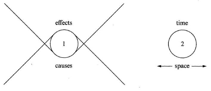
Figure 2.1: "Space-time location of causes and effects of events in region 1." (reproduced with permission from [8], pg. 239. Copyright Cambridge University Press. )

"The direct causes (and effects) of events are near by, and even the indirect causes (and effects) are no further away than permitted by the velocity of light. Thus for events in a space-time region 1 (…) we would look for causes in the backward light cone, and for effects in the future light cone. In a region like 2, space-like separated from 1, we would seek neither causes nor effects of events in 1. Of course this does not mean that events in 1 and 2 might not be correlated, as are the ringing of Professor Casimir’s alarm and the readiness of his egg. They are two separate results of his previous actions." ([8], pg. 239)

The above principle, Bell admits, "is not yet sufficiently sharp and clean for mathematics." He then considers the following as an implication of the principle above (with reference to Figure 2.2):

"A theory will be said to be locally causal if the probabilities attached to values of local beables in a space-time region 1 are unaltered by specification of values of local beables in a space-like separated region 2, when what happens in the backward light cone of 1 is already sufficiently specified, for example by a full specification of local beables in a space-time region 3…" ([8], pg. 239)

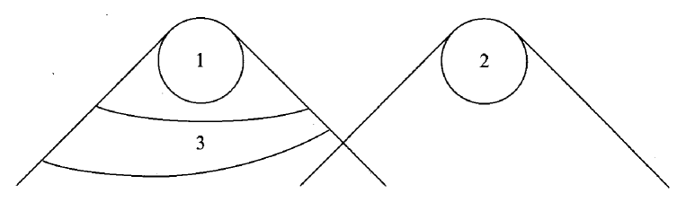
Figure 2.2: "Full specification of what happens in 3 makes events in 2 irrelevant for predictions about 1 in a locally causal theory." (reproduced with permission from [8], pg. 240. Copyright Cambridge University Press.)

The concept of "beable" was invented by Bell to contrast with the notion of "observable" that is fundamental in orthodox quantum mechanics:

"The beables of the theory are those elements which might correspond to elements of reality, to things which exist. Their existence does not depend on ‘observation’. Indeed observation and observers must be made out of beables." ([8], pg. 174)

The above and the specification in Bell’s formulation of local causality that the relevant beables are "local beables" are evidence that what he means by ‘local beables’ is precisely what I meant by ‘events’ in the previous section. I will stick to the latter terminology as it seems very non-problematic and familiar to physicists, who encounter the term with precisely this meaning in any undergraduate course in relativity.

We are now ready to formulate the principle mathematically:

Definition 1 (Local causality): A theory will be said to be locally causal iff for every pair of events $E_{1},\,E_{2}$ respectively contained in space-like separated regions 1 and 2, the probability, posited by the theory, of occurrence of event $E_{1}$ is independent of $E_{2}$, given the specification of some sufficient set of events $\mathcal{E}_{p1}$ in the past light cone of 1, i.e.,

$$P(E_{1}|E_{2},\mathcal{E}_{p1})=P(E_{1}|\mathcal{E}_{p1}).$$ (2.1)

It’s important to emphasise the need only for a sufficient set of events (and not necessarily the full specification of all events in the past light cone), for a reason which will be clear in the next section. What counts as a sufficient set of events will, of course, depend on the theory. The set of events in region 3 of Figure 2.2 would be sufficient in a theory where all causal chains are continuous. However, one can envisage theories in which that does not occur. This matter will not be too important for Bell’s theorem as the purpose of that will be to show that no such set can exist anywhere in the past light cone of $E_{1}$ and therefore that Local Causality fails.

2.3 Other general definitions

The previous Axioms and definitions were quite independent of any particular setup. To derive specific consequences of local causality we need to introduce some concrete experimental situation. The most common setting used in discussions of Bell’s theorem is constituted by two parties, traditionally called Alice and Bob, and this is the scheme of Figure 2.3. The definitions and theorems of this chapter will make use of that case only, but most of them could be generalised in an obvious way for arbitrary parties.

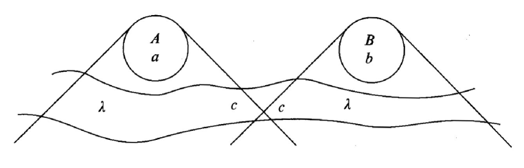
Figure 2.3: The bipartite experimental setup used for discussion of the concepts of this chapter. (reproduced with permission from [8], pg. 242. Copyright Cambridge University Press.)

• Alice and Bob are two spatially separated observers who can perform a number of measurements and observe their outcomes.

• For each pair of systems they perform measurements upon, the choices of measurement settings and their respective outcomes occur in regions which are space-like separated from each other, so that no signal travelling at a speed less than or equal to that of light could connect any two of them;

• For each pair of systems, we will denote by $a$ and $b$ Alice’s and Bob’s respective measurement settings, and by $A$ and $B$ their corresponding observed outcomes.

• Each pair of systems is prepared by an agreed-upon reproducible procedure $c$. The events corresponding to this preparation procedure are necessarily in the intersection of the past light cones of the measurements yielding $A$ and $B$;

• $a$, $b$, $A$, $B$ and $c$ represent events in the sense of the MRRF;

• $\lambda$ represents any further variables (in addition to $a$, $b$ and $c$) that may be relevant to the outcomes of the measurements considered, that is, conditioned upon which the probabilities of the experimental outcomes may be further specified. They are not fully determined by the preparation procedure $c$, and as such may be deemed "hidden variables". They are necessarily not known in advance, since any knowledge of additional variables could be assimilated into the preparation $c$. Conversely, if some of the variables associated with the preparation procedure are unknown, they must be assimilated into $\lambda$. In other words, the distinction between $c$ and $\lambda$ is merely epistemic, i.e., $c$ represents the set of known relevant variables and $\lambda$ represents the set of unknown (but not necessarily unknowable) relevant variables. Strictly speaking $\lambda$ describes a set of events in the union of the past light cones of the experiments as needed by Definition 1. However, one can also think of them as physical variables which are specified by those events;

• When an equation involving variables appears, it is to be understood that the equality holds for all values of those variables.

We can now specify the third axiom needed for Bell’s theorem.

Axiom 3 (External Conditionalisation, or Free will, or No backwards-causality): The choices of experiment $a$, $b$, can be conditioned on free variables uncorrelated with $\lambda$, such that knowledge of those choices does not provide any further information about the hidden variables, i.e., it does not change their probability distribution. Formally,

$$P(\lambda|a,b,c)=P(\lambda|c).$$ (2.2)

In other words, the choices can be freely made, independently of any relevant variables that influence the outcomes of the measurements under study. This is a fundamental requirement of any theory in which it is possible to separate the world into the system of interest and the rest of the world, where the rest of the world can be ignored as irrelevant to the evolution of the system. Some people may picture that as an allowance for the experimenters to make those choices at their own free will. This picture introduces the inconvenience of requiring us to explain what we mean by "free will", which is completely besides the point. Even if the world is completely deterministic and human free will is an illusion, External Conditionalisation would be an almost unavoidable assumption of any physical theory.

To make that clear, one can imagine that those choices are made by pointing photo-detectors at opposite parts of the sky and deciding based on fluctuations of the cosmic microwave background radiation; or that they depend on the output of a pseudo-random number generator; or that they are decided at the whim of an experimentalist; or by some further random quantum process, say, a measurement on a (presumably) uncorrelated spin-1/2 particle; or by any combination of those processes. This is where we see the importance of being clear about the need for the specification of only a sufficient set of events $\mathcal{E}_{p1}$ in the Definition 1. Of course the choices of experiment will depend on some events in the past light cone of the events under study, but a "superdeterministic" theory would be needed to entertain the possibility that the factors on which those choices depend can influence the evolution of the system under study. In such theory, any possible variable which one chooses to conditionalise the choices of experiment on would be statistically correlated with the set of hidden variables which are relevant to the experiments of Alice and Bob. And they would need to be conspiratorially correlated in such a way as to fool us into believing that local causality is violated by the correlations between those experiments while in reality the world is strictly locally causal.

That said, a possible way in which equation (2.2) could be violated is by way of backwards-in-time causality or retrocausality. Some authors [92] have claimed that in fact such backwards causality should be expected from the fact that fundamental physics is (mostly) time-symmetric, and could be the source of quantum nonlocality. This view, however, is far from being generally accepted.

Definition 2: A phenomenon is defined, for a given preparation procedure $c$, by the relative frequencies

$$f(A,B|a,b,c).$$ (2.3)

for all measurements $a$, $b$, and corresponding outcomes $A$, $B$.

The use of frequencies in that definition, instead of probabilities, is motivated by the fact that it is rather uncontroversial that frequencies are the things we observe, at least to an arbitrarily good approximation. Whether or not frequencies directly correspond to probabilities will depend on one’s interpretation of probabilities. Here we will make the distinction between the observable frequencies (the phenomenon) and the probabilities which are employed to predict or explain the phenomenon (the model). In general, models can make use of unobserved or even unobservable variables. Nevertheless, those variables can be taken to have an existence independent of observers, i.e., they can be taken to have an ontological status. Thus one can refer to such models as ontological models. The following is the most general kind of ontological model for the phenomena under consideration, in which the observed phenomena can be explained as arising out of our ignorance of underlying variables, where our ignorance is accounted for with standard probability theory, and where Axiom 3 holds.

Definition 3: An ontological model (or model in short) for a phenomenon consists of the set $\Lambda$ of values of $\lambda$, together with a probability distribution $P(\lambda|c)$ for every preparation procedure $c$ and a specification of

$$P(A,B|a,b,c,\lambda)$$ (2.4)

which predicts the phenomenon

$$\sum_{\lambda\in\Lambda}\,P(\lambda|c)\,P(A,B|a,b,c,\lambda)=f(A,B|a,b,c).$$ (2.5)

Nothing in the following discussions hangs on whether the $\lambda$ are discrete or continuous, so for simplicity I use discrete hidden variables. The above definition can be extended to a continuous set of hidden variables in the standard way.

Definition 4: An operational theory (OT) is the class of trivial models, i.e., the class of models for which

$$P(A,B,|a,b,c,\lambda)=f(A,B|a,b,c).$$ (2.6)

That is, in operational theories no hidden variables further specify the probabilities. One could argue that an operational theory contains no $\lambda$’s, but this definition, as a class of models with trivial dependences on $\lambda$, allows an operational theorist to talk about the $\lambda$’s even if they are not operationally meaningful.

Definition 5: A hidden variable model (HVM) is any model that is not trivial.

We will now determine what the Definition 1 of local causality implies to this experimental situation. Since $a$ and $A$ are space-like separated from $b$ and $B$, and the set of hidden variables completely specifies all relevant events in the past light cone of $a,\,A$ and $b,\,B$, we obtain

Corollary 1: A model is locally causal, i.e., a model satisfies local causality (LC) iff

$$P(A|a,b,B,c,\lambda)=P(A|a,c,\lambda),$$ (2.7)

plus the corresponding equations for $B$.

Definition 6: A model is said to be deterministic, or to satisfy determinism (D), iff

$$P(A,B|a,b,c,\lambda)\in\{0,1\}.$$ (2.8)

This implies that $A$ and $B$ are functions of the variables which condition those probabilities, i.e.,

$$A=A(a,b,c,\lambda),\;B=B(a,b,c,\lambda).$$ (2.9)

Definition 7: A model is said to be predictable, or to satisfy predictability (P) iff

$$P(A,B|a,b,c,\lambda)=P(A,B|a,b,c)\in\{0,1\}.$$ (2.10)

That is, a model is predictable iff it is trivial and deterministic. This implies that $A$ and $B$ are functions of

$$A=A(a,b,c),\;B=B(a,b,c).$$ (2.11)

This definition is motivated by the fact that the variables represented by $c$ are known. The former definition (determinism) is ontological (about how the world is), while this definition (predictability) is epistemic (about what one can know).

Definition 8: A phenomenon $\Phi_{1}$ associated with preparation $c_{1}$ is said to be irreducibly unpredictable, or to satisfy irreducible unpredictability (IU) iff it has no predictable models and there is no phenomenon $\Phi_{2}$ associated with a preparation $c_{2}=c_{1}\cup c^{\prime}$ (for all $c^{\prime}$) which has a predictable model and such that the frequencies $f_{1}$ of $\Phi_{1}$ are given by

$$f_{1}(A,B|a,b,c_{1})=\sum_{c^{\prime}}P(c^{\prime}|c_{1})P(A,B|a,b,c_{1},c^{\prime}),$$ (2.12)

where $P(A,B|a,b,c_{1},c^{\prime})\in\{0,1\}$.

In other words, a phenomenon is irreducibly unpredictable iff it has no predictable model and cannot be rendered predictable by knowledge of further variables. The reason for (2.12) is that the only way in which an unpredictable phenomenon could be rendered predictable without fundamentally changing the phenomenon would be if there were a deterministic hidden variable model which predicted the phenomenon, but for which the "hidden variables" could be in principle known in advance. But if the hidden variables were known in advance they could (in fact they should, since the only distinction between $\lambda$ and $c$, as mentioned before, is that the latter are known) be incorporated into the preparation variables. That is why I use the notation $c^{\prime}$ for those further knowable variables.

Definition 9: A model is said to satisfy locality (L) iff

$$P(A|a,b,c,\lambda)=P(A|a,c,\lambda),$$ (2.13)

plus the corresponding equation for $B$.

This was precisely the meaning that Bell intended for this term in his original 1964 paper [7], although without formal definition. Shimony called this parameter independence ([26], pg. 25).

Definition 10: A model is said to satisfy outcome independence (OI) iff

$$P(A|a,b,B,c,\lambda)=P(A|a,b,c,\lambda),$$ (2.14)

plus the corresponding equation for $B$.

This concept was introduced by Jarrett [59], under the misleading name of completeness. The present terminology is due to Shimony ([26], pg. 25). One could also consider calling it causality, so that local causality would be the conjunction of locality and causality. This choice would be justified if one takes causality to be a weakened form of determinism, in which the outcomes depend (maybe stochastically) only on the experimental settings, but not on the distant outcomes. In other words, in this view of causality the effects (the outcomes, things which are not controllable) at Alice’s can depend only on the local or distant causes (the settings, things which are controllable) but not on the distant effects. This terminology, however, would seem to rule out a common “explanation” of the quantum correlations: that the measurement on Bob’s system causes the quantum state to collapse which causes the outcomes at Alice to be what they are. This (non-relativistically invariant) causal picture would violate outcome independence since the collapsed quantum state depends on Bob’s outcome.

Definition 11: A model is said to be locally deterministic, or to satisfy local determinism (LD) iff it satisfies locality and determinism.

Definition 12: A model is said to violate p iff it lacks that property.

Definition 13: An operational theory is said to violate p iff all trivial models violate p.

Definition 14: A phenomenon is said to violate p iff all models violate p.

Definition 15: Nature is said to violate p iff a phenomenon violating p is observed.

2.4 General results

We now present the general results and relations (that is, those which are not specific to quantum mechanics) concerning the definitions of the previous section.

By the definition of conditional probability $P(A,B|a,b,c,\lambda)=P(A|B,a,b,c,\lambda)P(B|a,b,c,\lambda)$. Using Corollary 1 we arrive at

Theorem 1: Local causality is equivalent to factorisability, i.e.,

$$P(A,B|a,b,c,\lambda)=P(A|a,c,\lambda)P(B|b,c,\lambda).$$ (2.15)

Jarrett [59] showed that:

Theorem 2 (Jarrett 1984a): Local causality is the conjunction of locality and outcome independence.

The purpose of that decomposition was to argue that outcome independence was the concept to be blamed, while locality was the real consequence of relativity and therefore ought to be maintained. We’ll return to this important point later.

Theorem 3: Local causality is strictly stronger than locality.

That is, every locally causal model satisfies locality but not vice-versa. The proof is simple. Theorem 1 implies the first statement, and orthodox quantum mechanics provides an example of a model which satisfies locality but violates local causality.

Theorem 4: Determinism is strictly stronger than outcome independence.

If determinism holds, the outcome $A$ is fully determined by $(a,b,c,\lambda)$. Therefore knowledge of $B$ cannot change the probability of $A$ if $(a,b,c,\lambda)$ are specified, which is just the statement of outcome independence. To see the failure of the converse, just note that orthodox quantum mechanics for separable states violates determinism but satisfies outcome independence.

Corollary 2: Local determinism is strictly stronger than local causality.

This follows from the definition of local determinism and Theorems 2 and 4.

Theorem 5: Predictability is strictly stronger than determinism.

Every predictable model is obviously deterministic, but some deterministic models are not predictable. A trivial example is that of a deterministic model in which one does not know all relevant variables $\lambda$ (or does not know them precisely enough) but could know them in principle, (e.g. classical statistical mechanics), but there are models in which one cannot know all $\lambda$ even in principle (e.g. Bohmian mechanics).

Theorem 6: Some phenomena violate predictability.

Since the distinction between the hidden variables $(\lambda)$ and the variables that specify the preparation $(c)$ is an epistemic one, and since a phenomenon is defined partly by $c$, there are trivial examples of unpredictable phenomena — one just needs to ignore some relevant variables.

This does not imply that there are irreducibly unpredictable phenomena. I’ll return to this question later.

Theorem 7: No phenomenon violates determinism.

That doesn’t mean that no model violates determinism, but that every phenomenon has a possible model which satisfies determinism. To see that, define $\lambda_{0}$ and $\lambda_{1}$ by $P(A,B|a,b,c,\lambda_{0})=0$ and $P(A,B|a,b,c,\lambda_{1})=1$. Substituting in (2.5) we obtain $f(A,B|a,b,c)=P(\lambda_{1}|c)$, resulting in that every possible frequency can be modelled in this form. Of course, that leaves open the question of whether there really exist such events corresponding to the variables to play the role of $\lambda_{0}$ and $\lambda_{1}$, so one could read Theorem 7 as saying that it is impossible to prove that any phenomenon violates determinism.

Corollary 3: No phenomenon violates outcome independence.

Theorem 8 (Fine 1982): A phenomenon violates local determinism iff it violates local causality.

That is, any phenomenon that has a locally deterministic model has a locally causal model and vice versa. This theorem is due originally to Fine [41]. Note that this does not mean that all locally causal models are locally deterministic and vice versa (which in fact is false as per Corollary 2).

Proof. Any phenomenon that has a locally deterministic model automatically has a locally causal model, since all LD models are LC. To see the converse, remember that if there exists a locally causal model, the frequencies can be written as

$$f(A,B|a,b,c)=\sum_{\lambda}P_{LC}(\lambda|c)P_{LC}(A|a,c,\lambda)P_{LC}(B|b,c,\lambda).$$ (2.16)

We now add extra hidden variables for each of the factors on the right hand side, in a similar fashion as for the proof of Theorem 7. We decompose

$$P_{LC}(A|a,c,\lambda)=\sum_{\lambda_{A}}P^{\prime}(\lambda_{A}|c,\lambda)P_{LD}(A|a,c,\lambda_{A}),$$ (2.17)

where $P{}_{LD}(A|a,c,\lambda_{A})=\lambda_{A}\in\{0,1\}$. With a similar decomposition for $B$, we obtain

$$f(A,B|a,b,c) = \sum_{\lambda}P_{LC}(\lambda|c)P_{LC}(A|a,c,\lambda)P_{LC}(B|b,c,\lambda).$$

$$= \sum_{\lambda,\lambda_{A},\lambda_{B}}P_{LC}(\lambda|c)P^{\prime}(\lambda_{A},\lambda_{B}|c,\lambda)P_{LD}(A|a,c,\lambda_{A})P_{LD}(B|b,c,\lambda_{B})$$

$$= \sum_{\lambda^{\prime}}P_{LD}(\lambda^{\prime}|c)P_{LD}(A|a,c,\lambda^{\prime})P_{LD}(B|b,c,\lambda^{\prime}),$$

where we define $\lambda^{\prime}\equiv(\lambda,\lambda_{A},\lambda_{B})$ and $P_{LD}(\lambda^{\prime}|c)\equiv P_{LC}(\lambda|c)P^{\prime}(\lambda_{A},\lambda_{B}|c,\lambda)$, obtaining a locally deterministic model as desired.

2.4.1 Local causality and signalling

Bell was adamant in stressing that his concept of local causality was quite distinct from the concept of no faster than light signalling. One of the reasons for Bell’s rejection of the importance of the concept of signalling was that he understood that it was hard to talk about signalling without using anthropocentric terms like ‘information’ and ‘controllability’:

"Suppose we are finally obliged to accept the existence of these correlations at long range, (…). Can we then signal faster than light? To answer this we need at least a schematic theory of what we can do, a fragment of a theory of human beings. Suppose we can control variables like $a$ and $b$ above, but not those like $A$ and $B$. I do not quite know what ‘like’ means here, but suppose the beables somehow fall into two classes, ‘controllables’ and ‘uncontrollables’. The latter are no use for sending signals, but can be used for reception." ([8], pg.60)

But he rejects the idea that signal locality be taken as the fundamental limitation imposed by relativity:

"Do we have to fall back on ‘no signalling faster than light’ as the expression of the fundamental causal structure of contemporary theoretical physics? That is hard for me to accept. For one thing we have lost the idea that correlations can be explained, or at least this idea awaits reformulation. More importantly, the ‘no signalling…’ notion rests on concepts which are desperately vague, or vaguely applicable. The assertion that ‘we cannot signal faster than light’ immediately provokes the question:

Who do we think we are?

We who can make ‘measurements’, we who can manipulate ‘external fields’, we who can signal at all, even if not faster than light? Do we include chemists, or only physicists, plants, or only animals, pocket calculators, or only mainframe computers?" ([8], pg.245)

That is one of the reasons I have first presented the definition of local causality in a general context without the operational definitions used from Section 2.3 onwards. In Definition 1 no mention was made of measurements and outcomes, but only of events and space-time structure. We have then translated the consequences of that into our operational definitions with Corollary 1. But to even start talking about signalling, we need to have the operational model set up and explicit mention what are the controllable, uncontrollable and observable variables within it. This is precisely why Bell rejects the idea that this is a fundamental notion. I agree with Bell that if one wants to entertain the idea that signal locality is the fundamental restriction from relativity, one needs to put fundamental weight on epistemological terms. However, as long as one clearly understands that, I have no qualms with that position, in fact I find it an interesting possibility to pursue, and in this chapter it will lead to a nice new result.

Given the assumptions that the variables $a$ and $b$ are controllable (an assumption, in fact, already made in Axiom 3) we can formulate the concept of signal locality as follows.

Definition 16: A phenomenon is said to satisfy signal locality (SL) iff

$$f(A|a,b,c)=f(A|a,c),$$ (2.19)

plus the corresponding equation for $B$.

The reason is straightforward. If the phenomenon violates signal locality, then there exist at least two possible choices of setting $b$, $b^{\prime}$ such that $f(A|a,b,c)\neq f(A|a,b^{\prime},c)$. Therefore by looking at the frequency of outcomes of $A$ in a large enough ensemble (and in principle it is always possible for Alice to make all of the measurements in her ensemble space-like separated from all measurements in Bob’s ensemble), Alice can determine with arbitrary accuracy what setting Bob has chosen. Conditionalising this choice on a source of information, Bob can thereby send signals to Alice.

Definition 17: A model is said to satisfy signal locality (SL) iff the phenomena it predicts satisfies SL.

The reason behind Jarrett’s preference for locality (mentioned below Theorem 2) over outcome independence is that Jarrett believed that locality was equivalent to signal locality. However, that is an unwarranted assumption as argued by Maudlin [76]. The main counter-example is Bohmian mechanics. That theory violates L but not SL. The reason is that any attempt of controlling the distant outcome by the local choice of setting is thwarted by an unavoidable lack of knowledge of the hidden variables. On the other hand, if a model satisfies L it necessarily satisfies SL, as can be easily seen by substituting Eq. (2.13) in (2.5) and summing over $B$. In other words,

Theorem 9: :Locality is strictly stronger than signal locality.

While Jarrett’s rejection of models which violate locality is not well-grounded, his repulse of violations of locality is.

Theorem 10: A phenomenon violates locality iff it violates signal locality.

As argued above, if a phenomenon has a model which satisfies locality then the phenomena satisfies signal locality. The converse is also true: if a phenomenon satisfies signal locality then there is a model which satisfies locality: one example is the trivial model that corresponds to that phenomenon.

Theorem 11: If relativistic invariance is assumed, a phenomenon which violates signal locality will lead to contradictions.

Faster than light signalling can lead to paradoxes like the famous "grandfather paradox" of time travel — a time traveller goes to the past and kills his grandfather before his father was born, paradoxically thwarting the possibility of his own existence. Consider a scenario in which signal locality is violated by Alice’s and Bob’s experimental apparatuses such that $f(A_{1}|a_{1},b_{1},c_{1})\neq f(A_{1}|a_{1},b_{1}^{\prime},c_{1})$. How exactly these frequencies differ is unimportant, as Alice can always use an arbitrarily large ensemble such that $f(A_{1}^{\prime}|b_{1})\approx 1$ and $f(A_{1}^{\prime}|b_{1}^{\prime})\approx 0$, where $A_{1}^{\prime}$ is the event which corresponds to the frequency of the outcome $A_{1}$ within the ensemble being approximately $f(A_{1}|a_{1},b_{1},c_{1})$ and with good confidence distinct from $f(A_{1}|a_{1},b_{1}^{\prime},c_{1})$. Since $A_{1}^{\prime}$ and the choice between $b_{1}$ and $b_{1}^{\prime}$ are space-like separated, there exists a reference frame in which they occur simultaneously. If relativistic invariance is assumed, then it must be possible to produce, in any reference frame, a similar instantaneous signalling setup (otherwise there would be a preferred reference frame), and if we assume that there’s no preferred spatial direction for such signal transmission (if there were a preferred spatial direction, that would also be a violation of the principle of relativity), we can setup another pair of boxes where $f(B_{2}|a_{2},b_{2},c_{2})\neq f(B_{2}|a_{2}^{\prime},b_{2},c_{2})$. The choice $a_{2}/a_{2}^{\prime}$ of Alice’s experimental setting would be conditioned on $A_{1}^{\prime}$ (and therefore would be in the future light cone of $A_{1}^{\prime}$) and by use of a similar procedure as for the first setup, Alice and Bob arrange things such that $f(B_{2}^{\prime}|A_{1}^{\prime})\approx 1,\,f(B_{2}^{\prime}|\neg A_{1}^{\prime})\approx 0$, where ${}^{\prime}\neg^{\prime}$ denotes logical negation. Bob’s outcome $B_{2}^{\prime}$ is arranged to be in the past light cone of the choice between $b_{1}$ and $b_{1}^{\prime}$, and Bob conditions that choice such that he will choose $b_{1}^{\prime}$ if the result of measurement 2 is $B_{2}^{\prime}$, otherwise he will choose $b_{1}$. So we finally obtain the contradictory set of implications

$$b_{1} \Rightarrow A_{1}^{\prime}\Rightarrow B_{2}^{\prime}\Rightarrow b_{1}^{\prime}\Rightarrow\neg b_{1}$$

$$b_{1}^{\prime} \Rightarrow\neg A_{1}^{\prime}\Rightarrow\neg B_{2}^{\prime}\Rightarrow b_{1}\Rightarrow\neg b_{1}^{\prime}.$$ (2.20)

That is, if Bob chooses $b_{1}$, then he does not choose $b_{1}$, If Bob chooses $b_{1}^{\prime}$, then he does not choose $b_{1}^{\prime}$. So it is fair to say that relativity seems to exclude the possibility of violation of signal locality. Bell would say that this is not all it excludes, that relativity implies not simply signal locality but local causality. An interesting question is therefore whether violation of local causality by a phenomenon which does not violate signal locality can lead to such time travel paradoxes. If signal locality is satisfied, the above scenario cannot be set up, and the fact that we have observed violations of local causality (up to some loopholes) seems to point to the fact that no contradictions can arise out of that violation (inasmuch as a contradiction cannot be actually observed). However sensible this statement may sound, I can’t provide a proof to it. But it is interesting to mention it as a conjecture.

Conjecture 1: A phenomenon that violates local causality but not signal locality does not lead to contradictions even if relativistic invariance is assumed.

Remark 1: Nevertheless, a phenomenon that violates local causality is a non-local resource. That is, there are tasks Alice and Bob can do using this phenomenon that they could not do if they had access only to locally causal phenomena.

Theorem 12: For a phenomenon to violate locality it is necessary and sufficient for the operational theory to violate locality.

This follows directly from Theorem 10 and the definitions of operational theory and signal locality.

Theorem 13: For a phenomenon to violate local causality it is necessary but not sufficient for the operational theory to violate local causality.

The necessary part is obvious. We can show insufficiency by appealing to a counter-example: single particle quantum mechanics restricted to measurements of position. The operational theory violates local causality (see Theorem below) but there’s a locally causal model for the phenomena involved: single-particle Bohmian mechanics.

Remark 2: Thus, unlike locality, to say whether a phenomenon violates local causality it is necessary to consider hidden variable models.

2.5 Quantum Results

Definition 18: Orthodox quantum theory or operational quantum theory (OQT) is an operational theory in which

$$P(A,B|a,b,c,\lambda)=Tr[\hat{\Pi}_{A}\otimes\hat{\Pi}_{B}\rho_{c}],$$ (2.21)

where $\hat{\Pi}_{A}$ is a projector onto the subspace corresponding to outcome $A$ of observable $\hat{a}$ and similarly for $B$, while $\rho_{c}$ is a positive unit-trace operator associated with the preparation $c$.

Definition 19: A quantum model is a model whose predictions agree with OQT.

Definition 20: A quantum phenomenon is a phenomenon predicted by OQT.

Theorem 14 (Einstein 1927): OQT violates local causality.

This was first proved by Einstein at the 1927 Solvay conference [119]. Consider a single particle with a position wavefunction spread out over space, and consider $a$ as a measurement of the particle position in the region around Alice and similarly for Bob. Then the probability that Alice finds the particle in her region is not independent of whether Bob finds the particle in his region. And since in OQT there are no hidden variables, (2.7) is not satisfied.

Theorem 15 (Heisenberg 1930): OQT does not violate locality.

This is a well-known result that arises out of the fact that operators corresponding to measurements in spatially separated regions commute. In his 1930 book [54], Heisenberg replied to Einstein’s objection to OQT above by pointing out that the theory would not allow faster-than-light signalling.

Corollary 4: Quantum phenomena do not violate signal locality.

Theorem 16 (Jarrett 1984b): OQT violates outcome independence.

This is a consequence of Jarrett’s Theorem 2, and Theorems 14 and 15.

2.5.1 The EPR argument

As we mentioned above, in 1927 Einstein had already shown that OQT violated local causality (the term wasn’t used until Bell, but Einstein clearly stated that quantum mechanics "contradicts the principles of relativity" [120]). That was always intended by Einstein as a proof that OQT was incomplete, i.e., that there must be further hidden variables beyond the quantum state to completely specify the properties of physical systems.

Einstein’s 1927 argument however is not as widely recognised as the Einstein, Podolsky and Rosen (EPR) argument of 1935 [39]. Maybe because the argument in that paper was more well articulated, maybe because in the Solvay conference Einstein also tried to prove quantum mechanics to be inconsistent — not only incomplete — by carefully set-up thought experiments. Those attempts were thwarted by Bohr, who argued that Einstein was not consistently using the uncertainty principle at all levels in his analysis of the experiments. The physics community largely takes Bohr to have triumphed over Einstein on those arguments, and therefore Einstein’s failure on that front would have been automatically transferred to his 1927 theorem about local causality.

In a recent paper [57], Harrigan and Spekkens suggest that Einstein himself preferred the (more complicated) argument for incompleteness using entangled states. More precisely, Einstein’s preferred argument was that used in a 1935 correspondence with Schrödinger, not the EPR argument which — those authors claim — does not reflect precisely Einstein’s opinion on the matter. The reason for that preference, they argue, is that this argument not only rules out the completeness of quantum mechanics (if one assumes local causality, of course), but also it provides an extra argument for the view that the quantum states are merely epistemic in nature.

Another reason for preference of the EPR argument, mentioned in [120] and [57] over Einstein’s 1935 is an experimental one: the measurement statistics used in the 1927 argument can be trivially simulated with a mixed state, while those of the EPR argument cannot. The critics could evade the earlier argument by denying the coherence of the state upon which the measurements are performed, a move that cannot be made in the later.

But the most likely reason, in my opinion, for the community’s recognition of the EPR argument over the 1927 one is that the former also substantially differs from the later in that it introduces entangled states. Even if EPR failed in convincing the community of the incompleteness of orthodox quantum mechanics, the kind of states they considered opened the door to Bell’s recognition of the failure of one of EPR’s premises instead — local causality — and from there lead to the multiple applications in the modern field of quantum information science. They also influenced Schrödinger to envisage his infamous "cat paradox" [104] (and to coin the term ‘entanglement’ to refer to the strange kind of states EPR consider).

EPR’s argument is essentially that given (i) a suitable necessary condition for completeness of a theory; (ii) an apparently reasonable sufficient condition for determining when a physical variable corresponds to an "element of physical reality"; (iii) the assumption of local causality; and (iv) some predictions of quantum mechanics concerning entangled states; one must conclude that quantum mechanics is incomplete, in the sense that there must exist hidden variables to further specify physical states. I won’t go into the EPR argument in detail here, however, as it will be the subject of Chapter 3.

2.5.2 Bell’s Theorems

We now arrive at the famous Bell theorems. By 1964 it was known that OQT violates local causality, but one could still imagine, as EPR did, that a more detailed description of the phenomena was possible in which local causality was maintained. Bell’s startling contribution was to show that this hope was futile. The importance of this theorem cannot be overemphasised. It has even been dubbed the "most profound discovery of science" [111]. In 1964, however, Bell did not prove the stronger theorem about local causality, but only a weaker version:

Theorem 17 (Bell 1964): All deterministic quantum models violate locality.

In other words, quantum phenomena violate local determinism. By Fine’s Theorem 8 this is equivalent to the strong form of Bell’s theorem:

Theorem 18 (Bell 1971): Quantum phenomena violate local causality.

However, that was not fully recognised until much later. In 1964 Bell was considering locality and not local causality, as is evident by this passage:

"It is the requirement of locality, or more precisely that the result of a measurement on one system be unaffected by operations on a distant system with which it has interacted in the past, that creates the essential difficulty." ([7], pg. 14)

and that he considers only deterministic hidden variables is clear in the following discussion of the specific setup:

"The result $A$ (…) is then determined by $a$ and $\lambda$, and the result $B$ (…) is determined by $b$ and $\lambda$, and $A(a,\lambda)=\pm 1,\,B(b,\lambda)=\pm 1$. The vital assumption is that the result $B$ (…) does not depend on the setting $a$, (…) nor$A$ on $b$." ([7], pg. 15)

In a 1971 paper ([8], pg. 37), Bell considered a model which allowed some "indeterminism with a certain local character" associated with the detectors — essentially a factorisable model with arbitrary probabilities, which by Theorem 1 follows from local causality — so this could be taken as the first clear proof of Theorem 18. But he did not clearly use the term local causality with the meaning of Definition 1 until 1976 ([8], pg. 54).

While in hindsight Bell’s 1964 and 1971 theorems are logically equivalent (by way of Theorem 8), the 1964 theorem could not be directly applied to experimental situations, since it assumed perfect correlations (which are obviously not observable in any real experiment). The Bell inequality of 1971 however (essentially a version of the Clauser, Horne, Shimony, Holt (CHSH) inequality of 1969 [24], but which was derived from a local deterministic model) is applicable to real experimental situations. Many experiments realised since then strongly follow the quantum mechanical predictions, and (up to some loopholes involving detection efficiencies and/or lack of space-like separation) support the conclusion

Conclusion 1: Nature violates local causality.

2.5.3 Determinism and Predictability

Theorem 19 (Born): OQT violates determinism.

This is essentially the content of Born’s postulate that the modulus square of the wave function corresponds to probabilities of outcomes of measurements, the extension of which for mixed states is given by (2.21). Since for any state (determined by a preparation $c$) there is at least one measurement for which the probabilities are different from $1$ or $0$, determinism is violated by OQT.

Corollary 4: OQT violates predictability.

Corollary 5: Quantum phenomena violate predictability.

That is a consequence of Corollary 4 plus the fact that the definition of predictability implies that if a model is not predictable, then the phenomena it predicts violates predictability. This still does not mean that quantum phenomena are irreducibly unpredictable, that is, it doesn’t mean that there cannot be further knowable variables such that the phenomena would be rendered predictable. That there are no such further knowable variables is essentially the content of Heisenberg’s Uncertainty Principle (HUP), that is,

Theorem 20 (Heinsenberg 1926): Quantum phenomena are irreducibly unpredictable.

But the proof of Heisenberg’s uncertainty principle, based on the commutation relations between different observables, can only be made within quantum mechanics. Bohmian mechanics is deterministic but also not predictable, but again those facts are model-dependent. The definition of quantum phenomenon is "a phenomenon predicted by OQT". OQT states that some phenomena are irreducibly unpredictable (by way of HUP), but OQT could be wrong about that. However, Theorem 7 (which states that no phenomenon violates determinism) may be taken to imply that nothing can be said about predictability in a model-independent way.

This debate was in the centre of the famous Einstein-Bohr debates starting in the Solvay conference of 1927. Einstein was then unsatisfied with the indeterminism of quantum mechanics and attempted to show that it was inconsistent by devising clever gedanken experiments aiming to break Heisenberg’s Uncertainty Principle. But Bohr thwarted every such attempt by pointing a flaw in Einstein’s reasoning. History is one the side of Bohr who is widely regarded as the victor of those debates. Einstein’s flaw was essentially to ignore the uncertainty principle for some variables, which would allow him to obtain more knowledge than permitted by OQT for some other variables. Bohr’s reply was to point that if the principle was observed consistently throughout the problem, Einstein’s move would fail. However, of course, Bohr could never prove that OQT was correct and that the HUP must always hold, all he did was point out that OQT was consistent. There is no question about that, but could he give a better argument to convince Einstein that OQT was correct about that? On this question I offer the following theorem.

Theorem 21: If relativistic invariance is assumed, Nature is irreducibly unpredictable or some observed phenomena can lead to contradictions.

The contradictions in question are just those involved in the grandfather-type paradox considered in Theorem 11. The proof is simple. Suppose Nature is not irreducibly unpredictable, i.e., that for any observed phenomenon there is a possible trivial deterministic model that reproduces the phenomenon as in (2.12). By Theorem 17 there are phenomena for which there is no local deterministic model, therefore any such deterministic model must be nonlocal. However, since the models under consideration are trivial, if they are nonlocal the phenomena they predict must violate signal locality. Therefore if those phenomena are not irreducibly unpredictable then they violate signal locality and by Theorem 11 will lead to contradictions if relativistic invariance is assumed. Moreover, such phenomena violating local determinism have been observed, therefore if Nature is not irreducibly unpredictable then some observed phenomena can lead to contradictions (if one obtains the hitherto hidden but observable information to render the phenomena predictable).

In the last of Einstein’s thought experiments, Bohr’s reply made use of Einstein’s own General Theory of Relativity to reject Einstein’s thought experiment. Of course, Einstein or Bohr were not aware of Bell’s Theorem, but interestingly, if they were, Bohr could, by the use of Einstein’s Special Theory, have convinced Einstein not only that OQT was consistent, but that Nature is irreducibly unpredictable regardless of quantum mechanics.

Conclusion 2: The above definitions and theorems imply the following structure in phenomenon space (PS):

$$vSL = vL\subset vLD=vLC\subset PS,$$

$$\{\} = vD\subset vP\subset PS$$ (2.22)

Here $\{\}$ denotes the empty set, vSL denotes the set of phenomena violating signal locality, and similarly for vL, vLC, vLD, vD and vP.

2.6 Making sense of it

In the beginning of this Chapter I indicated that there are, still today, many discussions about what Bell’s theorem(s) prove and what concepts it requires us to give up. Here I’ll sketch a few of those debates and what we can conclude about them in light of the careful definitions and theorems of this chapter.

2.6.1 Locality and outcome independence

I have already mentioned Jarrett’s preference of rejecting outcome independence and keeping locality. The motivation is essentially Theorems 9 and 10, which state that violation of locality by a phenomenon will lead to paradoxes if relativistic invariance is assumed. However, before rushing into conclusions, we must remember that the concept of a phenomenon violating a property is quite distinct from that of a model lacking that property. In fact, we have seen that it is possible for a model to violate locality while the related phenomena do not. So keeping locality does not necessarily lead to paradoxes. A desire to avoid paradoxical situations is not sufficient reason to reject locality.

Bell’s theorem states that quantum phenomena violate local causality. Heisenberg’s Theorem 15 says that quantum phenomena do not violate locality. One could take that to mean that quantum phenomena violate outcome independence. But by Corollary 3, it is impossible for any phenomenon to violate outcome independence. The choice will depend on the model. Some models respect locality but not OI, such as OQT. Some respect OI but not locality, such as Bohmian mechanics. Some respect neither, as Nelson’s mechanics. Bell’s theorem says that none can respect both.

2.6.2 Determinism and hidden variables

There’s a common misconception in the literature about Bell inequalities which maintains that what Bell’s theorem tells us to give up is determinism and/or hidden variables. That probably arises from the fact that the original 1964 Bell theorem (and many subsequent derivations) was in fact about the failure of local determinism, that is, the conjunction of locality and determinism. For a reader who was already used to the violation of determinism by orthodox quantum mechanics, and who didn’t notice the fact that violation of locality by a model did not imply (the truly objectionable) violation of signal locality, the choice seemed clear. And since the early models did not mention the possibility of nondeterministic hidden variables, it is understandable if those readers then took Bell’s theorem as definitive proof of the failure of the project of hidden variables.

Curiously, that was quite the opposite from Bell’s intent. Bell was a supporter of the hidden variable program, and his purpose was to show that it was not fair to reject Bohmian mechanics — the leading contender among the hidden variable theories — due to its nonlocality, since that was an unavoidable feature of any hidden variable model.

In any case, we now know that what is at stake is not just local determinism, but the weaker concept of local causality. And by Remark 2, to even consider the concept of a phenomenon violating local causality, one needs to consider hidden variable theories. And even if one has other reasons to reject hidden variables, one cannot avoid the fact that OQT violates local causality. In other words, rejecting determinism and/or hidden variables does not make the world an entirely local place.

A common reason for rejecting hidden variables, Bohmian mechanics in particular, is that this theory is deterministic but does not allow predictability. If the hidden variables exist, why can’t we know about them? Theorem 21, while not directly answering the question, points out to the fact that (unless relativistic invariance is violated) Nature is irreducibly unpredictable, so that this problem is not exclusive of Bohmian mechanics (just as nonlocality, Bell showed, isn’t either).

With no intention of being a supporter of hidden variables, it’s interesting to point out that there are other reasons to consider them: they are potential solutions to the measurement problem, in that they do not make ‘measurement’ a fundamental feature of the world like OQT, they make sense of quantum cosmology, and they allow an ignorance interpretation of probabilities.

2.6.3 Reality

Finally, some theorists defend the idea that what violations of Bell’s inequalities tell us to give up is realism. These people take the term ’local realism’ to be a conjuntion of ’locality’ and ’realism’, and favour to reject the latter. We can identify four main views in which such a conjunction, in our terminology, can consistently be taken. In the first, Axioms 1 to 3 are accepted implicitly and realism is equated with hidden variables. This view, therefore, falls under the same criticism pointed out in 2.6.2. In the second, Axioms 1 to 3 and the possibility of HVs are accepted implicitly, but one equates ’realism’ with outcome independence or determinism. This would make sense if one believes that the only acceptable hidden variable models are those that are deterministic, or at least that satisfy outcome independence. Then one can consistently reject ’realism’ in this sense and keep locality. However, the holder of this view cannot escape the fact that local causality is still violated by OQT. In a third possibility, Axioms 1 to 3 are accepted implicilty, all the concepts defined through use of an ontological model are put under the label ’realism’, and ’locality’ is taken to mean signal locality. In this view, therefore, ’locality’ is not violated, and one refuses to talk about anything that goes under the name ’realism’. This, however, cannot be more than a form of operationalism, for which the only escape from the fact that OQT violates local causality would be to hold that local causality is not an interesting concept.

A fourth possibility is to reject Axioms 1 or 2. However, the motivation for that cannot be simply the desire to keep local causality, because the MRRF had to be assumed before one can even define local causality. So a theorist who chooses to reject realism probably has other motivations than simply to save local causality.

That said, there are possible moves in that direction. A popular one is Everett’s (or Many-Worlds) interpretation [40], which maintains that there is in reality a single, unitarily-evolving, wave function for the universe (or multiverse?). Therefore in a sense all possible outcomes of all experiments (and of all particle interactions throughout the universe for that matter) occur. Axiom 2 is clearly violated. Axiom 1 is not necessarily violated, since events really occur somewhere in the multiverse independently of observers. It’s just that we don’t have direct access to all of them.

Yet another possibility is to maintain a relational view of quantum states, along the lines supported for example by Rovelli in [100]. In this view, quantum states are always relative to an observer or reference frame. It is possible that different observers will disagree about whether or not some events occur, and in a relational world there’s no matter of fact about such events independently of any observer. Axiom 1 is clearly violated. Axiom 2 may or may not be, depending on how one pursues the idea. It is possible that relational quantum theories of gravity (i.e., of space-time geometry) will also reject it. To emphasise the meaning of a violation of Axiom 1, let me be explicit: in a fully relational theory, it is possible that the very existence of events are not absolute facts independent of reference frames. This would be a startling conclusion, far beyond the mere relativity of space and time which we have come to accept and — dare I say — understand. Can reality itself be relative? Although this idea goes dangerously close to a radical solipsism, a more moderate reading may be possible. In special relativity, the fact that lengths or time lapses are relative does not entail that they don’t exist — they just have this previously unsuspected property. In the same vein, to say that events are relative to reference frames does not entail that they don’t exist — again, it is just another surprising property. However, I would say that although it is intriguing, whether the whole idea ultimately makes sense (and most importantly, whether it can lead to new predictions) remains to be seen.

Chapter 3 The EPR paradox and Steering

As outlined in Section 2, in a seminal 1935 paper, Einstein, Podolsky and Rosen (EPR) [39] demonstrated an inconsistency between the premises that go under the name of local realism and the notion that quantum mechanics is complete. EPR never regarded it as a paradox, but as an argument to prove the incompleteness of quantum mechanics. The name ‘paradox’ was probably introduced by those who could not believe with EPR that quantum mechanics was indeed incomplete but could not see a flaw in the argument either. In hindsight, we now know (since Bell) that, while the argument is sound, one of the premises — local causality — is false. However, we will retain the historically prevalent term ‘paradox’. Our reasons to study the EPR paradox are threefold.

Firstly, we aim to do historical justice to EPR and put their argument in their correct standing, distilling its essence and formalising it to make it clear how it relates to the notion of local causality as used in discussions of Bell’s theorem and to the notion of entanglement or quantum non-separability.

Secondly, we will see that the EPR paradox can be demonstrated in a loophole-free way with current technology, thereby providing conclusive evidence of the failure of its underlying premises, as opposed to the current situation with Bell inequalities, as pointed out in Chapter 1 on page 1.

Thirdly, we will relate the EPR paradox to the concept of steering originally defined by Schrödinger [104] in a reply to EPR and recently formalised by Wiseman and co-authors [121], confirming the latter’s claim that any demonstration of the EPR paradox is also a demonstration of steering. We will further show that the converse is also true: any demonstration of steering is also a demonstration of the EPR paradox. With reference to that work we will then see that the EPR paradox (or steering) constitutes a new class of (non-)locality intermediate between the classes of quantum (non-)separability and Bell (non-)locality. This classification could prove important in the context of Quantum Information Processing, therefore it is desirable to formulate criteria to determine to which classes a given state (or a set of correlations) belongs.

The original EPR paradox was based on position and momentum observables. Bohm [14] extended the example of EPR to the case of discrete observables, particularly to the case of two spin-1/2 particles. That is the version that was used by Bell in deriving his famous inequalities and it has played a central role in our understanding of quantum entanglement. Both the original argument of EPR and Bohm’s version, however, rely on perfect correlations, which are obviously experimentally unattainable. That situation was corrected by Margaret Reid in 1989 [96], when she derived experimental criteria for demonstration of the EPR paradox which were applicable to realistic situations where noise and losses are inevitable. The Reid criteria are a standard tool in Quantum Optics, and have been used for demonstrations of the EPR paradox with continuous-variables [84, 132, 109, 17, 53] where quadrature measurements play the role of the position and momentum observables.

However, there is to date no such tool for the case of discrete observables. Experiments by Wu and Shaknov [123] gave evidence for discrete EPR correlation, but because detection efficiencies were extremely low, only a small fraction of emitted pairs were detected, meaning that “no-enhancement” assumptions [30] were incorporated.

We will derive new criteria that can be applied to discrete observables, both for the case originally envisaged by Bohm and to other classes of states, even in presence of inefficiencies in the preparation or detection procedures. The extent to which these inefficiencies are allowed will be studied in detail. Using one of these criteria, we show that the loop-hole free demonstration of the EPR-Bohm paradox is predicted for considerably lower detection efficiencies than required for Bell’s theorem. This disparity is even more striking in the case of macroscopic fields, where we propose for feasible efficiencies to demonstrate a type of EPR-Bohm correlation from which one can deduce existence of mesoscopic and macroscopic quantum superpositions.

While not enough to falsify EPR’s local realism, the proposed EPR paradox experiments do demonstrate a particularly strong form of entanglement. For this EPR-entanglement, local realism can only be reconciled with quantum mechanics if one accepts the existence of an underlying localised hidden variable (non-quantum) state. Put another way, if one can accept only quantum states, then the EPR correlation implies nonlocal effects.

3.1 The Einstein-Podolsky-Rosen argument

We will start with a detailed analysis of the original EPR argument, before finding a suitable mathematical formulation of it. The EPR paper starts with a distinction between reality and the concepts of a theory, followed by a critique of the operationalist position, clearly aimed at the views advocated by Bohr, Heisenberg and the other proponents of the Copenhagen school.

"Any serious consideration of a physical theory must take into account the distinction between the objective reality, which is independent of any theory, and the physical concepts with which the theory operates. These concepts are intended to correspond with the objective reality, and by means of these concepts we picture this reality to ourselves.

In attempting to judge the success of a physical theory, we may ask ourselves two questions: (1) ‘Is the theory correct?’ and (2) ‘Is the description given by the theory complete?’ It is only in the case in which positive answers may be given to both of these questions, that the concepts of the theory may be said to be satisfactory. The correctness of the theory is judged by the degree of agreement between the conclusions of the theory and human experience." [39]

Any theory will have some concepts which will be used to aid in the description and prediction of the phenomena which are their subject matter. In quantum theory, Schrödinger introduced the concept of the wave function and Heisenberg described the same phenomena with the more abstract matrix mechanics. EPR argue that we must distinguish those concepts from the reality they attempt to describe. One can see the physical constructs of the theory as mere calculational tools if one wishes, but those authors warn that one must be careful to avoid falling back into a pure operationalist position; the theory must strive to furnish a complete picture of reality.

In Chapter 2, we argued that a minimal realist-relativistic framework for physical theories, and certainly the position advocated by Einstein, can be represented by the conjunction of Axioms 1 and 2 of that chapter, namely that the existence of physical events is independent of observers or reference frames and that those events can be associated to points in a relativistic space-time. This framework makes explicit, as EPR desired, that events are among those things which are part of the "objective reality, which is independent of any theory". With that framework in place, we can abstract out any specific concepts of a theory and represent the most fundamental aspects of any description of a phenomenon by what was termed an ‘ontological model’ or simply ‘model’. EPR’s requirement that the theory is correct is built into Definition 2 of a model by requiring that it correctly predicts the phenomenon. Their requirement that it be complete will be addressed within the ontological model shortly. But first let us look at the rest of EPR’s argument.

EPR follow the previous considerations with a necessary condition for completeness:

EPR’s necessary condition for completeness: "Whatever the meaning assigned to the term complete, the following requirement for a complete theory seems to be a necessary one: every element of the physical reality must have a counterpart in the physical theory." [39]

Soon afterwards they note that this condition only makes sense if one is able to decide what are the elements of the physical reality. Contrary to a common belief, they did not then attempt to define element of physical reality. Instead, they provide a sufficient condition of reality:

EPR’s sufficient condition for reality: "The elements of the physical reality cannot be determined by a priori philosophical considerations, but must be found by an appeal to results of experiments and measurements. A comprehensive definition of reality is, however, unnecessary for our purpose. We shall be satisfied with the following criterion, which we regard as reasonable. If, without in any way disturbing a system, we can predict with certainty (i.e., with probability equal to unity) the value of a physical quantity, then there exists an element of physical reality corresponding to this physical quantity." [39]

Later in the same paragraph it is made explicit that this criterion is "regarded not as a necessary, but merely as a sufficient, condition of reality". This is followed by a discussion that, in quantum mechanics, if a system is in an eigenstate of an operator $A$ with eigenvalue $a$, by this criterion, there must be an element of physical reality corresponding to the physical quantity $A$. "On the other hand", they continue, if the state of the system is a superposition of eigenstates of $A$, "we can no longer speak of the physical quantity $A$ having a particular value". After a few more considerations, they state that "the usual conclusion from this in quantum mechanics is that when the momentum of a particle is known, its coordinate has no physical reality". We are left therefore, according to EPR, with two alternatives:

EPR’s dilemma: "From this follows that either (1) the quantum-mechanical description of reality given by the wave function is not complete or (2) when the operators corresponding to two physical quantities do not commute the two quantities cannot have simultaneous reality." [39]

They justify this by reasoning that "if both of them had simultaneous reality — and thus definite values — these values would enter into the complete description, according to the condition for completeness". And in the crucial step of the reasoning: "If then the wave function provided such a complete description of reality it would contain these values; these would then be predictable [my emphasis]. This not being the case, we are left with the alternatives stated". Brassard and Méthot [13] have pointed out that strictly speaking EPR should conclude that (1) or (2), instead of either (1) or (2), since they could not exclude the possibility that (1) and (2) could be both correct. However, this does not affect EPR’s conclusion. It was enough for them to show that (1) and (2) could not both be wrong, and therefore if one can find a reason for (2) to be false, (1) must be true.

The next section in EPR’s paper intends to find a reason for (2) to be false, that is, to find a circumstance in which one can say that there are simultaneous elements of reality associated to two non-commuting operators. They consider a composite system composed of two spatially separated subsystems $S_{A}$ and $S_{B}$ which are prepared, by way of a suitable initial interaction, in an entangled state of the type

$$|\Psi\rangle=\sum_{n}c_{n}|\psi_{n}\rangle_{A}\otimes|u_{n}\rangle_{B},$$ (3.1)

where the $|\psi_{n}\rangle_{A}$ denote a basis of eigenstates of an operator, say $\hat{O}_{1}$, of subsystem $S_{A}$ and $|u_{n}\rangle_{B}$ denote some (normalised but not necessarily orthogonal) states of $S_{B}$. If one measures the quantity $\hat{O}_{1}$ at $S_{A}$, and obtains an outcome corresponding to eigenstate $|\psi_{k}\rangle_{A}$ the global state is reduced to $|\psi_{k}\rangle_{A}\otimes|u_{k}\rangle_{B}$. If, on the other hand, one chooses to measure a non-commuting observable $\hat{O}_{2}$, with eigenstates $|\phi_{s}\rangle_{A}$, one should instead use the expansion

$$|\Psi\rangle=\sum_{s}c^{\prime}_{s}|\phi_{s}\rangle_{A}\otimes|v_{s}\rangle_{B},$$ (3.2)

where $|v_{s}\rangle_{B}$ represent another set of normalised states of $S_{B}$. Now if the outcome of this measurement is, say, the one corresponding to $|\phi_{r}\rangle_{A}$, the global state is thereby reduced to $|\phi_{r}\rangle_{A}\otimes|v_{r}\rangle_{B}$. Therefore, "as a consequence of two different measurements performed upon the first system, the second system may be left in states with two different wave functions". This is just what Schrödinger later termed steering, and we’ll return to that later. Now enters the crucial assumption of locality.

EPR’s locality assumption: "Since at the time of measurement the two systems no longer interact, no real change can take place in the second system in consequence of anything that may be done to the first system." [39]

"Thus", conclude EPR, "it is possible to assign two different wave functions to the same reality". They now consider a specific example where those different wave functions are eigenstates of two non-commuting operators. If the initial state was of type

$$\Psi(x_{A},x_{B})=\int_{-\infty}^{\infty}e^{ix{}_{A}p/\hbar}e^{-ix{}_{B}p/\hbar}dp,$$ (3.3)

then if one measures momentum $\hat{p}^{A}$ at $S_{A}$ and finds outcome $p$, the reduced state of subsystem $S_{B}$ will be the one associated with outcome $-p$ of $\hat{p}^{B}$. On the other hand, if one measures position $\hat{x}^{A}$ and finds outcome $x$, the reduced state of $S_{B}$ will be the one corresponding to outcome $x$ of $\hat{x}^{B}$. By measuring position or momentum at $S_{A}$, one can predict with certainty the outcome of the same measurement on $S_{B}$. But $\hat{p}^{B}$ and $\hat{x}^{B}$ correspond to non-commuting operators. EPR conclude from this that

"In accordance with our criterion of reality, in the first case we must consider the quantity [$\hat{p}^{B}$] as being an element of reality, in the second case the quantity [$\hat{x}^{B}$] is an element of reality. But, as we have seen, both wave functions [corresponding to $-p$ and $x$] belong to the same reality." [39]

In other words, by using the sufficient condition for reality, the assumption of locality and the predictions for the entangled state under consideration, EPR conclude that there must be elements of reality associated to a pair of non-commuting operators. So the (2) horn of EPR’s dilemma proved before is closed, leaving as the only alternative option (1), namely, that the quantum mechanical description of physical reality is incomplete.

In hindsight, as we now know that the premise of locality is not entirely justified, we can read EPR’s argument as demonstrating the incompatibility between the premises of locality, the completeness of Quantum Mechanics and some of its predictions. However, one could block the conclusion of the argument by rejecting those statistical predictions required to formulate the argument. This move is particularly easy to be made since the necessary predictions are of perfect correlations, unobtainable in practice due to unavoidable inefficiency in preparation and detection of real physical systems. This problem was considered by W. H. Furry already in 1936 [43] but experimentally useful criteria for the EPR paradox were only proposed in 1989 by Margaret Reid [96].

3.2 The EPR-Reid criterion

The essential difference in the derivation of the EPR-Reid criteria [96] and the original EPR argument is in a modification of the sufficient condition for reality. This could be stated as the following:

Reid’s sufficient condition of reality: If, without in any way disturbing a system, we can predict with some specified uncertainty the value of a physical quantity, then there exists a probabilistic element of physical reality which determines this physical quantity with at most that specific uncertainty.

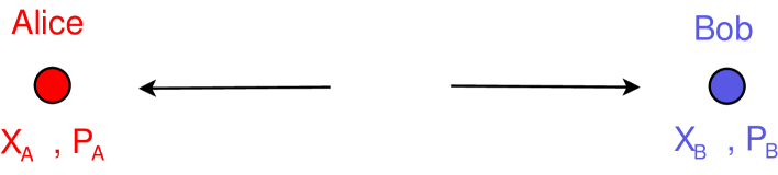
Figure 3.1: The EPR scenario. Alice and Bob are two spatially separated observers who can perform one of two (position or momentum) measurements available to each of them.

The scenario considered is the same as the one for the EPR paradox above, as depicted in Fig. 3.1, but one does not need a state which predicts the perfect correlations considered by EPR. Instead, the two experimenters, Alice and Bob, can measure the conditional probabilities of Bob finding outcome $x_{B}$ in a measurement of $\hat{x}_{B}$ given that Alice finds outcome $x_{A}$ in a measurement of $\hat{x}_{A}$, i.e., $P(x_{B}|x_{A})$. Similarly they can measure the conditional probabilities $P(p_{B}|p_{A})$ and the unconditional probabilities $P(x_{A})$, $P(p_{A})$. We denote by $\Delta^{2}(x^{B}|x^{A})$, $\Delta^{2}(p^{B}|p^{A})$ the variances of the conditional distributions $P(x_{B}|x_{A})$, $P(p_{B}|p_{A})$, respectively. Reid now defines the average inference variances

$$\Delta_{inf}^{2}(x^{B}|\hat{x}^{A}) = \sum_{x^{A}}P(x^{A})\Delta^{2}(x^{B}|x^{A})$$

$$\Delta_{inf}^{2}(p^{B}|\hat{p}^{A}) = \sum_{p^{A}}P(p^{A})\Delta^{2}(p^{B}|p^{A}).$$ (3.4)

The notation $\Delta_{inf}^{2}(x^{B}|\hat{x}^{A})$ is to indicate the average inference variance of $x^{B}$ given that Alice measures $\hat{x}^{A}$ and similarly for $p^{B}$. Reid argues, by use of the sufficient condition of reality above, that since Alice can, by measuring either position $\hat{x}^{A}$or momentum $\hat{p}^{B}$, infer with some uncertainty $\Delta_{inf}(x^{B}|\hat{x}^{A})$ or $\Delta_{inf}(p^{B}|\hat{p}^{A})$ the outcomes of the corresponding experiments performed by Bob, and since by the locality condition of EPR her choice cannot affect the elements of reality of Bob, then there must be simultaneous probabilistic elements of reality which determine $\hat{x}^{B}$ and $\hat{p}^{B}$ with at most those uncertainties. Now by Heisenberg’s Uncertainty Principle (HUP), quantum mechanics imposes a limit to the precision with which one can assign values to observables corresponding to non-commuting operators $\hat{x}$ and $\hat{p}$. In appropriately rescaled units the relevant HUP reads $\Delta x\Delta p\geq 1$. Therefore, if quantum mechanics is complete as defined by EPR and the locality condition holds, by use of the adapted sufficient condition of reality, the limit with which one could determine the average inference variances above is

$$\Delta_{inf}(x^{B}|\hat{x}^{A})\Delta_{inf}(p^{B}|\hat{p}^{A})\geq 1.$$ (3.5)

This is the EPR-Reid criterion. Violation of that criterion signifies the EPR paradox. It has been used in experimental demonstration with continuous-variables [84, 132, 109, 17, 53] where quadrature measurements play the role of the position and momentum observables.

3.3 Formalising EPR

I will now propose a mathematical formalisation of the premises of the EPR argument following the formalism of Chapter 2.

It is evident that EPR had well in mind the basic Axioms of the MRRF defined on page 2.1. We have already argued in 3.1 that the first of EPR’s desiderata, "Is the theory correct?", is taken care of automatically by the definition of a ‘model’, since it is required that it correctly predicts the phenomenon under study. So we can now use the ontological model to formalise the rest of their premises.

3.3.1 The original argument

Let us first understand what EPR’s sufficient condition of reality amounts to. It is a criterion which, when satisfied, assigns a physical variable to the set of variables which have an "element of reality" associated to them. Let us denote this set by $\mathcal{ER}$. The setup of the ontological model is essentially the same as that considered by EPR, so by EPR’s sufficient condition of reality, if after the measurement of an observable $a$ in which outcome $A$ is obtained, one deduces that the probability of now obtaining $B$ in a measurement of $b$ is unity, then there’s an element of reality associated to $b$.

Definition 1 (EPR’s sufficient condition of reality) If the outcome of measurement $b$ is predictable given the outcome of measurement $a$, then there’s an element of reality associated to $b$, i.e.,

$$P(B|A,a,b,c)\in\{0,1\}\rightarrow b\in\mathcal{ER}.$$ (3.6)

The necessary condition for completeness is not so transparent. It is a priori not obvious what EPR had in mind by "a counterpart in the physical theory". However, we can extract the meaning by looking at when they actually use that condition. It is just in the justification of what I’ve called EPR’s dilemma, already mentioned in Section 3.1 3.1: "If then the wave function provided such a complete description of reality it would contain these values; these would then be predictable" [my emphasis]. In other words, it is necessary, for EPR, that the variables corresponding to elements of reality be predictable by the wave function if it provides a complete description of reality. The wave function is fully specified by the preparation procedure, so denoting, following EPR, $C(OQT)\equiv$"the quantum-mechanical description of reality given by the wave function is complete" we obtain

Definition 2 (EPR’s necessary condition for completeness) If the quantum mechanical description of reality given by the wave function is complete, then if there’s an element of reality associated to $b$, the value $B$ of $b$ given only the preparation procedure must be predictable, i.e.

$$C(OQT)\rightarrow(b\in\mathcal{ER}\rightarrow P(B|b,c)\in\{0,1\}).$$ (3.7)

We can now derive EPR’s dilemma. Assume $C(OQT)$ and take two non-commuting observables $b$ and $b^{\prime}$. If there’s an element of reality associated with both of them, then by Definition 2 they must both be predictable. But we know by the HUP that no quantum model involving non-commuting operators is predictable. Therefore there cannot be elements of reality associated to both of two non-commuting operators. Denote this last statement $NC$. Then $C(OQT)\rightarrow NC$, which is logically equivalent to $\neg C(OQT)\vee NC$. EPR’s dilemma can now be stated as

Theorem 1 (EPR’s dilemma) If the quantum mechanical description of reality given by the wave function is complete, then there cannot be elements of reality associated to both of two non-commuting operators.

Now enters the example of the entangled state. With that state, one can find observables $b$, $b^{\prime}$, $a$, $a^{\prime}$ such that $P(B|A,a,b,c)\in\{0,1\}$ and that $P(B^{\prime}|A^{\prime},a^{\prime},b^{\prime},c)\in\{0,1\}$. Let us denote this observation $ENT$. Given $ENT$ and Definition 1, there must be elements of reality associated to both $b$ and $b^{\prime}$, i.e., $b,b^{\prime}\in\mathcal{ER}$. This is where the locality assumption enters the reasoning in a fundamental way, by requiring that the elements of reality at $B$ do not depend on the choice of experiment at $A$. Definition 1 used that implicitly by not mentioning that one should actually carry out the measurements under consideration, only that one would be able to predict the outcome of $b$ (or $b^{\prime})$ if one decided to measure $a$ (or $a^{\prime}$). Close to the end of their paper, EPR remark that

"One could object to this conclusion on the grounds that our criterion of reality is not sufficiently restrictive. Indeed, one would not arrive at our conclusion if one insisted that two or more physical quantities can be regarded as simultaneous elements of reality only when they can be simultaneously measured or predicted. […] This makes the reality of $P$ and $X$ depend upon the process of measurement carried out on the first system, which does not disturb the second system in any way. No reasonable definition of reality could be expected to permit this." [39]

Therefore given the observation of $ENT$ and Definition 1, there must be elements of reality associated to both non-commuting operators, and the consequent of Theorem 1 is false. Therefore the antecedent must be false, and EPR conclude, quantum mechanics is incomplete.

Theorem 2 (the EPR argument) The sufficient condition of reality and some predictions of quantum mechanics imply that the quantum mechanical description of reality is incomplete.

3.3.2 General formalisation

We can understand what kind of locality EPR had in mind if we revisit their condition for completeness. In Definition 2 we see that if there’s an element of reality associated to $b$, and quantum mechanics is complete, then the outcome of $b$ given the quantum state must be predictable. They implicitly mean that if there’s an element of reality associated to a variable, then if one had the knowledge of enough facts about the system one would be able to predict the outcome of a measurement of that observable with certainty. In the language of the ontological model of Chapter 2, this means that there must be a deterministic hidden variable model for the outcome of $b$. With this consideration Definition 1 implies (I remind the reader that the expressions are to be understood as valid for all values of the variables, including $\lambda$)

$$P(B|A,a,b,c)\in\{0,1\}\rightarrow b\in\mathcal{ER}\rightarrow P(B|b,c,\lambda)\in\{0,1\},$$ (3.8)

Now it is obvious that

$$P(B|A,a,b,c)\in\{0,1\}\rightarrow P(B|A,a,b,c,\lambda)\in\{0,1\},$$ (3.9)

and to obtain (3.8) from (3.9) we just need the assumption of local causality as defined in Chapter 2, which we reproduce here for completeness:

Corollary 1: A model is locally causal, i.e., a model satisfies local causality (LC) iff

$$P(B|A,a,b,c,\lambda)=P(B|b,c,\lambda),$$ (3.10)

plus the corresponding equations for $A$.

So the locality concept that goes into Definition 1 is that of local causality. Remember that this implies that the joint probabilities factorise, i.e., that any model that satisfies local causality must have the form

$$f(A,B|a,b,c)=\sum_{\lambda\in\Lambda}\,P(\lambda|c)\,P(A|a,c,\lambda)P(B|b,c,\lambda).$$ (3.11)

What about completeness? If Orthodox Quantum Theory is complete, then for pure states it is essentially the assumption that there are no hidden variables. No possible new information could change the probability assigned to the outcomes of measurements. Since hidden variables could be unknowable by any observer even in principle, such as is the case in Bohmian mechanics, a more correct statement would be that no actual variables exist in the past light cones of the measurements under study such that, conditionalised on those variables, the probabilities of the outcomes of said measurements would be further specified. Formally, that means that if OQT is complete, then the probabilities of Bob’s outcome, say, can only be those allowed by quantum states $P_{Q}(B|b,c,\lambda)=Tr[\hat{\Pi}_{B}\rho_{c,\lambda}^{B}].$ I use the subscript $Q$ to indicate quantum probabilities, where $\hat{\Pi}_{B}$ is a projector onto the subspace corresponding to outcome $B$ of observable $\hat{b}$ while $\rho_{c,\lambda}^{B}$ is a positive unit-trace operator for subsystem $B$ associated with the preparation $c$ and with the unknown variable $\lambda$. This is a strong constraint, since by Heisenberg’s Uncertainty Principle, not all probabilities are allowed to be associated simultaneously to two non-commuting operators $\hat{b}$ and $\hat{b}^{\prime}.$ By those considerations, we arrive at the first main result of this Chapter.

Proposition 1: The conjunction of local causality and completeness implies

$$f(A,B|a,b,c)=\sum_{\lambda\in\Lambda}\,P(\lambda|c)\,P_{Q}(A|a,c,\lambda)P_{Q}(B|b,c,\lambda).$$ (3.12)

This is equivalent to the statement that there exists a separable (i.e., non-entangled) state which correctly describes the phenomenon. An entangled, or non-separable [117] quantum state $\rho$ for two subsystems A and B, is one which cannot be written as a convex combination of product states, i.e., as

$$\rho=\sum_{i}\eta_{i}\rho_{i}^{A}\otimes\rho_{i}^{B},$$

where the $\eta_{i}$ are probabilities, i.e., they are real non-negative numbers and $\sum_{i}\eta_{i}=1,$ and $\rho_{i}^{A}$ and $\rho_{i}^{B}$ are quantum states for subsystems A and B respectively. The consequence has not been widely recognised before and deserves to be emphasised.

Any proof that a phenomenon cannot be described by a separable state is proof that the phenomenon violates the conjunction of local causality and completeness of operational quantum theory.

That is, the conjunction of local causality and completeness of quantum theory, the basic premises of the EPR argument, can be shown to be inconsistent with observation without the need for EPR’s sufficient condition of reality. The reason is that (3.12) is the most general model which is compatible with both of these premises, allowing for the most general distribution of local elements of reality which are compatible with the assumption that operational quantum theory is complete.

However, the EPR argument was asymmetric in that it considered the effect of knowledge of the outcomes of measurements on one side of the apparatus, say Alice’s, on the state on the other side, say Bob’s. Schrödinger called this effect steering, and that arguably reflects the spirit of the EPR paradox more closely than the general nonseparability of (3.12). We will therefore use the term EPR paradox to refer to this particular kind of violation of local causality and completeness, and not the general violation of 3.12. This is the topic of the next subsection.

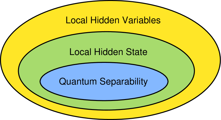
Figure 3.2: The hierarchy of locality models. The diagram depicts the ’state space’, that is, the space of possible quantum states. If a certain state is separable then all measurements that can be performed on it have a LHS model and if it has a LHS model then it will have a LHV model, but the converse implications do not hold.

3.3.3 The connection with Steering

Suppose we assume completeness of OQT for Bob’s subsystem, but do not restrict the hidden variables in Alice’s side in any way. That implies

Proposition 2: The conjunction of local causality and completeness for Bob’s subsystem implies

$$f(A,B|a,b,c)=\sum_{\lambda\in\Lambda}\,P(\lambda|c)\,P(A|a,c,\lambda)P_{Q}(B|b,c,\lambda).$$ (3.13)

This was termed a Local Hidden State (LHS) model by Wiseman and co-authors [121], and was proposed as a formalisation of the concept of steering, which can best be described in the quantum information fashion, that is, as a task.

The task is the following. Alice wants to convince Bob that she can act on his state, or steer it, at a distance. If Bob does not trust Alice and believes he has a local quantum state, he will believe that the measurement statistics of their experimental outcomes will be given by (3.13), since that is the most general way in which his local quantum state can be classically correlated with Alice’s measurement outcomes. Therefore if by looking at Alice’s and his own joint measurement probabilities, Bob cannot find a model of form (3.13), he’ll be convinced that Alice’s choice of experiment can somehow steer his own state.

In that letter, Wiseman et al. answered a few questions about steering. They have demonstrated that, as applied to states, the concept of Bell non-locality, or the inexistence of a Local Hidden Variable (LHV) model, is strictly stronger than steerability and steerability is strictly stronger than non-separability, that is, that if a quantum state demonstrates Bell non-locality then it necessarily demonstrates steering but not vice-versa, and if it demonstrates steering it necessarily demonstrates non-separability, but not vice-versa. This hierarchy is schematised in Fig. 3.2.

Here we will be interested in a different question. Our purpose is to experimentally demonstrate steering, which by the preceding arguments represent a demonstration of the EPR paradox. When do the experimental outcomes violate (3.13)? We want to find clear experimental signatures, in the form of inequalities, which, when violated, imply steering or the EPR paradox. We’ll first show that the LHS model directly imply the EPR-Reid criterion for continuous-variables, and then we’ll derive new criteria for the EPR-Bohm paradox.

3.3.4 The EPR-Reid criterion re-derived

It is easy to show that for the original EPR state, the measurement outcomes cannot be described in the form (3.13), To see that, note that for all $\lambda$, Alice can choose to measure $a$ or $a^{\prime}$ and thereby predict with certainty either $b$ or $b^{\prime}.$ But the value of $\lambda$ is independent of Alice’s choice. So for all $\lambda$, the outcomes of $b$ and $b^{\prime}$ must be determined, that is, it must be simultaneously the case that $P_{Q}(B|b,c,\lambda)\in\{0,1\}$ and $P_{Q}(B|b^{\prime},c,\lambda)\in\{0,1\}$. But no quantum state allows that probability assignment, and therefore the LHS model cannot describe the joint statistics.

But in the laboratory there are no such perfect correlations. What about the more general case of imperfect detection and preparation efficiencies? And what about other states which do not predict such correlations even with perfect efficiencies?

Recall that we defined, for the situation considered in Section 3.2, average inference variances as $\Delta_{inf}^{2}(x^{B}|\hat{x}^{A})=\sum_{x^{A}}P(x^{A})\Delta^{2}(x^{B}|x^{A}),\>\Delta_{inf}^{2}(p^{B}|\hat{p}^{A})=\sum_{p^{A}}P(p^{A})\Delta^{2}(p^{B}|p^{A}).$ Consider the LHS model of (3.13), which applied to the situation at hand reads (omitting henceforth unnecessary notation)

$$P(x^{A},x^{B})=\sum_{\lambda\in\Lambda}\,P(\lambda)\,P(x^{A}|\lambda)P_{Q}(x^{B}|\lambda).$$ (3.14)

The conditional probability distribution of $x^{B}$ given an outcome $x^{A}$ of $\hat{x}^{A}$ is then

$$P(x^{B}|x^{A})=\sum_{\lambda\in\Lambda}\frac{P(\lambda)\,P(x^{A}|\lambda)}{P(x^{A})}P_{Q}(x^{B}|\lambda).$$ (3.15)

It is a general result that if a probability distribution can be written in the form of a convex combination of further normalised probability distributions,

$$P(z)=\sum_{i}P(i)P(z|i),$$ (3.16)

then the variance of the resulting combination is larger than or equal to the combination of the variances, i.e.,

$$\Delta^{2}z\geq\sum_{i}P(i)\Delta^{2}(z|i).$$ (3.17)

Eq. (3.13) has the form of (3.16), so the variance $\Delta^{2}(x^{B}|x^{A})$ of the conditional distribution (3.15) must satisfy the inequality

$$\Delta^{2}(x^{B}|x^{A})\geq\sum_{\lambda}\frac{P(\lambda)\,P(x^{A}|\lambda)}{P(x^{A})}\Delta_{Q}^{2}(x^{B}|\lambda),$$ (3.18)

where $\Delta_{Q}^{2}(x^{B}|\lambda)$ represents the variance of $P_{Q}(x^{B}|\lambda).$ Substituting (3.18) into the definition of $\Delta_{inf}^{2}(x^{B}|\hat{x}^{A})$ we obtain

$$\Delta_{inf}^{2}(x^{B}|\hat{x}^{A}) \geq \sum_{\lambda,x^{A}}P(x^{A})\frac{P(\lambda)\,P(x^{A}|\lambda)}{P(x^{A})}\Delta_{Q}^{2}(x^{B}|\lambda)$$ (3.19)

$$= \sum_{\lambda}P(\lambda)\Delta_{Q}^{2}(x^{B}|\lambda).$$

A similar procedure produces the equivalent inequality for $\Delta_{inf}^{2}(p^{B}|\hat{p}^{A})$. We now define two vectors

$$u = (\sqrt{P(\lambda_{1})}\Delta_{Q}(x^{B}|\lambda_{1}),\,\sqrt{P(\lambda_{2})}\Delta_{Q}(x^{B}|\lambda_{2}),...)$$

$$v = (\sqrt{P(\lambda_{1})}\Delta_{Q}(p^{B}|\lambda_{1}),\,\sqrt{P(\lambda_{2})}\Delta_{Q}(p^{B}|\lambda_{2}),...),$$ (3.20)

and note that $\sum_{\lambda}P(\lambda)\Delta_{Q}^{2}(x^{B}|\lambda)=|u|^{2}$ and similarly for $p^{B}$ and $v$. By use of the Cauchy-Schwarz inequality, i.e., $|u||v|\geq u\cdot v$ we obtain

$$\Delta_{inf}^{2}(x^{B}|\hat{x}^{A})\Delta_{inf}^{2}(p^{B}|\hat{p}^{A}) \geq \sum_{\lambda}P(\lambda)\Delta_{Q}^{2}(x^{B}|\lambda)\sum_{\lambda^{\prime}}P(\lambda^{\prime})\Delta_{Q}^{2}(p^{B}|\lambda^{\prime})$$ (3.21)

$$= |u|^{2}|v|^{2}\geq(u\cdot v)^{2}$$

$$= \left\{\sum_{\lambda}P(\lambda)\Delta_{Q}(x^{B}|\lambda)\Delta_{Q}(p^{B}|\lambda)\right\}^{2}.$$

Now remember that $\Delta_{Q}(x^{B}|\lambda)$ and $\Delta_{Q}(p^{B}|\lambda)$ represent standard deviations over the same quantum state $\rho_{\lambda}^{B}.$ Therefore they must obey the HUP

$$\Delta_{Q}(x^{B}|\lambda)\Delta_{Q}(p^{B}|\lambda)\geq 1,$$ (3.22)

and by substituting (3.22) in (3.21) we finally arrive at the EPR-Reid criterion

$$\Delta_{inf}(x^{B}|\hat{x}^{A})\Delta_{inf}(p^{B}|\hat{p}^{A})\geq 1.$$ (3.23)

So we see that we can derive the EPR-Reid criterion directly from the premises of local causality and completeness, which imply the LHS model. No additional condition of reality is necessary.

3.4 Criteria for the EPR-Bohm paradox

In Bohm’s EPR paradox, spin measurements $J_{\theta}^{A}$ and $J_{\phi}^{B}$ are performed, simultaneously, on two spatially separated subsystems, $A$ and $B$. For the quantum states

$$|\psi_{j}\rangle=\frac{1}{\sqrt{2j+1}}\sum_{m=-j}^{j}(-1)^{j-m}|j,m\rangle_{A}|j,-m\rangle_{B}$$ (3.24)

there is a maximum correlation between the results if the same spin component is measured at each location. Here $|j,m\rangle_{A/B}$ are the eigenstates of $J^{2}$ and $J_{z}$ respectively, for $A/B$. Opposite outcomes are predicted for $J_{\theta}^{A}$ and0 $J_{\theta}^{B}$, so that the outcome of measurement of any one of $J_{x}^{B}$, $J_{y}^{B}$, $J_{z}^{B}$ can be predicted, with absolute certainty, by measurement of one of the $J_{x}^{A}$, $J_{y}^{A}$, $J_{z}^{A}$. Bohm’s original variant [14] of the EPR argument considered only the Bell-state $|\psi_{1/2}\rangle.$

The EPR-Bohm argument follows analogously to the EPR argument analysed before in this Chapter, except that instead of being based in the uncertainty principle for position-momentum, it is based on that for the spin observables, as depicted in Fig. 3.3.

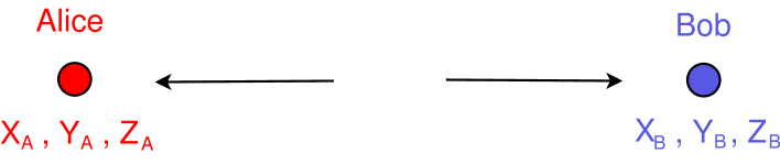
Figure 3.3: The EPR-Bohm scenario. Alice and Bob are two spatially separated observers who can perform one of three spin measurements available to each of them.

One of the uncertainty relations that impose lower bounds on the uncertainties for spin observables is of the form

$$\Delta j_{x}^{B}\Delta j_{y}^{B}\geq|\langle j_{z}^{B}\rangle|/2.$$ (3.25)

The lower case $j_{\theta}$ indicate the outcomes of measurements $J_{\theta}$.

To derive experimental criteria for the EPR-Bohm paradox, we define the measurable average inference variance in the prediction of $J_{\phi}^{B}$, based on measurement $J_{\theta}^{A}$ at $A$ [96].

$${\normalcolor\Delta_{est}^{2}j_{\phi}^{B}=\langle(j_{\phi}^{B}-j_{\phi|\theta,est}^{B})^{2}\rangle\geq\sum_{j_{\theta}^{A}}P(j_{\theta}^{A})\Delta^{2}(j_{\phi}^{B}|j_{\theta}^{A})=\Delta_{inf}^{2}(j_{\theta}^{B}|J_{\phi}^{A})}$$ (3.26)

Here $j_{\phi|\theta,est}^{B}$ is an inferred estimate for $j_{\phi}^{B}$, given an outcome $j_{\theta}^{A}$ for $J_{\theta}^{A}$, and the average is over all outcomes $j_{\phi}^{B}$, $j_{\theta}^{A}$. The inequality follows because, for a given $j_{\theta}^{A}$, the estimate that minimises $\langle(j_{\phi}^{B}-j_{\phi|\theta,est}^{B})^{2}\rangle$ is the mean of $P(j_{\phi}^{B}|j_{\theta}^{A})$. This minimum is optimal, but not always accessible, in EPR experiments. From now on we will derive everything for the $\Delta_{inf}^{2}(j_{\theta}^{B}|J_{\phi}^{A})$, but one should keep in mind that one can measure the less optimal but possibly more accessible $\Delta_{est}^{2}j_{\phi}^{B}$, modifying the inequalities in an obvious way.

We will use a technique similar to that used to re-derive the EPR-Reid criterion in the previous section. We first assume that the measurement statistics can be described by a LHS model, which implies

$$\Delta_{inf}^{2}(j_{\theta}^{B}|J_{\phi}^{A})\geq\sum_{\lambda}P(\lambda)\Delta_{Q}^{2}(j_{\theta}^{B}|\lambda),$$ (3.27)

for all $\theta$, $\phi$, by an entirely analogous reasoning as in the derivation of (3.19).

We now again define two vectors

$$u = (\sqrt{P(\lambda_{1})}\Delta_{Q}(j_{x}^{B}|\lambda_{1}),\,\sqrt{P(\lambda_{2})}\Delta_{Q}(j_{x}^{B}|\lambda_{2}),...)$$

$$v = (\sqrt{P(\lambda_{1})}\Delta_{Q}(j_{y}^{B}|\lambda_{1}),\,\sqrt{P(\lambda_{2})}\Delta_{Q}(j_{y}^{B}|\lambda_{2}),...),$$ (3.28)

and by using the Cauchy-Schwarz inequality

$$\Delta_{inf}^{2}(j_{x}^{B}|J_{x}^{A})\Delta_{inf}^{2}(j_{y}^{B}|J_{y}^{A}) \geq \sum_{\lambda}P(\lambda)\Delta_{Q}^{2}(j_{x}^{B}|\lambda)\sum_{\lambda^{\prime}}P(\lambda^{\prime})\Delta_{Q}^{2}(j_{y}^{B}|\lambda^{\prime})$$

$$\geq \left\{\sum_{\lambda}P(\lambda)\Delta_{Q}(j_{x}^{B}|\lambda)\Delta_{Q}(j_{y}^{B}|\lambda)\right\}^{2}.$$

But in this case the relevant uncertainty relation is

$$\Delta_{Q}(j_{x}^{B}|\lambda)\Delta_{Q}(j_{y}^{B}|\lambda)\geq\frac{1}{2}|\langle j_{z}^{B}|\lambda\rangle|,$$ (3.30)

where $\langle j_{z}^{B}|\lambda\rangle$ represents the average of $J_{z}^{B}$ over the quantum state $\rho_{\lambda}^{B}$. By substituting (3.30) in (3.4)

$$\Delta_{inf}(j_{x}^{B}|J_{x}^{A})\Delta_{inf}(j_{y}^{B}|J_{y}^{A})\geq\frac{1}{2}\sum_{\lambda}P(\lambda)|\langle j_{z}^{B}|\lambda\rangle|.$$ (3.31)

Now note that further specifying the hidden variables cannot decrease the average of the modulus of the mean, so that

$$\sum_{\lambda}P(\lambda)|\langle j_{z}^{B}|\lambda\rangle|\geq\sum_{j_{z}^{A}}P(j_{z}^{A})|\langle j_{z}^{B}|j_{z}^{A}\rangle|\geq|\langle j_{z}^{B}\rangle|$$ (3.32)

and finally we arrive at the following theorem.

Theorem 3: The following inequality if violated for spatially separated systems A and B would demonstrate Bohm’s EPR paradox

$$\Delta_{inf}(j_{x}^{B}|J_{x}^{A})\Delta_{inf}(j_{y}^{B}|J_{y}^{A})\geq\sum_{j_{z}^{A}}P(j_{z}^{A})|\langle j_{z}^{B}|j_{z}^{A}\rangle|.$$ (3.33)

We reiterate that the choice of measuring $J_{x}^{A}$, for example, to infer $j_{x}^{B}$ was purely conventional. It will be the best choice in a state of type (3.24), but nothing special hangs on which particular quantum observable actually corresponds to what we called $J_{x}^{A}$, $J_{y}^{A}$ $J_{z}^{A}$. In a practical situation one should choose whichever observables optimise the violation of (3.33). The observables at $B$, however, must actually correspond to three mutually orthogonal directions, as the uncertainty principle used is only valid in that situation.

We point out that, from (3.32), $\Delta_{inf}(j_{x}^{B}|J_{x}^{A})\Delta_{inf}(j_{y}^{B}|J_{y}^{A})<|\langle j_{z}^{B}\rangle|/2$ also signifies the EPR paradox, as shown by Bowen et al [16], who demonstrated this inequality experimentally for Stokes operators [66] that represent the polarisation of optical fields. For the states (3.24), $\langle j_{Z}^{B}\rangle=0$ and this latter form is not useful.

The states (3.24) violate (3.33) and can be investigated experimentally using parametric down conversion [72]. We re-express (3.24) using Schwinger’s formalism

$${\normalcolor{\color[rgb]{1,0,0}{\normalcolor|\psi_{j}\rangle}}} = \frac{1}{N!\sqrt{N+1}}(a_{+}^{\dagger}b_{-}^{\dagger}-a_{-}^{\dagger}b_{+}^{\dagger})^{N}|0\rangle,$$ (3.34)

where $a_{\pm}$ are boson operators for orthogonally-polarised field modes of $A$, a similar set is defined for $B$, $j=N/2$ (where here $j$ represents the eigenvalues of $J^{2}$ as in state (3.24)) and $|0\rangle$ is the multi-mode vacuum. We define the Schwinger spin operators

$$J_{x}^{A} = \frac{1}{2}\left(\hat{a}_{-}\hat{a}_{+}^{\dagger}+\hat{a}_{-}^{\dagger}\hat{a}_{+}\right)$$

$$J_{y}^{A} = \frac{1}{2i}\left(\hat{a}_{-}\hat{a}_{+}^{\dagger}-\hat{a}_{-}^{\dagger}\hat{a}_{+}\right)$$

$$J_{z}^{A} = \frac{1}{2}\left(\hat{a}_{+}^{\dagger}\hat{a}_{+}-\hat{a}_{-}^{\dagger}\hat{a}_{-}\right)$$

$$N^{A} = \left(\hat{a}_{+}^{\dagger}\hat{a}_{+}+\hat{a}_{-}^{\dagger}\hat{a}_{-}\right).$$ (3.35)

The situation of the EPR-Bohm setup is therefore extended with number measurements, as in Fig. 3.4.

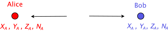
Figure 3.4: The extended EPR-Bohm scenario. Alice and Bob are two spatially separated observers who can perform one of four measurements (one of three "spin" components or a total number measurement) available to each of them.

Fields $a_{\pm}$ and $b_{\pm}$ are spatially separated, and impinge on polarising beam splitters to enable a measure of the photon number differences, $J_{z}^{A}$ and $J_{z}^{B}$, the spin measurements $J_{x/y}^{A}$, $J_{x/y}^{B}$ being made with phase shifts that immediately precede the polariser.

A case of experimental interest is $j=1/2$, the Bell state, but with detection efficiency $\eta$, so that there is a non-zero probability ($1-\eta$) of photons not being detected. The outcome of no detection corresponds to $0$ for both $\hat{a}_{+}^{\dagger}\hat{a}_{+}$ and $\hat{a}_{-}^{\dagger}\hat{a}_{-}$ and hence $0$ for $J_{\theta}^{A}$ (similarly for $J_{\phi}^{B}$). Calculation reveals

$$\Delta_{inf}^{2}(j_{x}^{B}|j_{x}^{A})=\Delta_{inf}^{2}(j_{y}^{B}|j_{y}^{A})=\eta(1-\eta^{2})/4$$ (3.36)

and

$$\sum_{j_{z}^{A}}P(j_{z}^{A})|\langle j_{z}^{B}|j_{z}^{A}\rangle|=\eta^{2}/2,$$ (3.37)

so the paradoxical correlations are obtained where $\eta>0.62$. This is consistent with the Werner state [117]

$$\rho_{w}=(1-p_{s})\frac{\mathbb{I}}{4}+p_{s}|\psi_{1/2}\left\rangle\right\langle\psi_{1/2}|$$ (3.38)

($\frac{\mathbb{I}}{4}$ is the maximally mixed density operator) which yields the EPR paradox when $p_{s}>0.62$. Entanglement occurs when, and only when, $p_{s}>0.33$, so the EPR paradox is more difficult to confirm [17, 121].

The states (3.34) can be generated using two parametric amplifiers [30] as modelled by the interaction Hamiltonian

$$H=i\hbar\kappa(a_{+}^{\dagger}b_{-}^{\dagger}-a_{-}^{\dagger}b_{+}^{\dagger})-i\hbar\kappa(a_{+}b_{-}-a_{-}b_{+})$$ (3.39)

Assuming the initial state to be a vacuum, the solution after a time $t$ is a superposition of the (3.34). The predictions of a particular $|\psi_{j}\rangle$ could be tested by restricting to the ensemble with a fixed $N^{B}$. Most interesting is the limit of large $\langle N^{B}\rangle$. We therefore propose to detect the Bohm-EPR correlation using the full solution of $H$. For macroscopic systems, measurement of all the conditional probabilities can be difficult. We present an alternative Bohm-EPR criterion.

Theorem 4: Violation of the following inequality for spatially separated $A$ and $B$ reveals an EPR paradox

$$\Delta_{inf}^{2}(j_{x}^{B}|J_{x}^{A})+\Delta_{inf}^{2}(j_{y}^{B}|J_{y}^{A})+\Delta_{inf}^{2}(j_{z}^{B}|J_{z}^{B})\geq\frac{\langle N^{B}\rangle}{2}$$ (3.40)

The proof is analogous to that of (3.33), except that we follow [115, 58] to write a quantum uncertainty relation

$$\Delta^{2}j_{x}^{B}+\Delta^{2}j_{y}^{B}+\Delta^{2}j_{z}^{B}\geq\Delta^{2}N^{B}/4+\langle N^{B}\rangle/2.$$ (3.41)

Inequality (3.40) is tested for (3.39), with detection efficiency $\eta$. The $\Delta_{est}^{2}j_{\theta}^{B}$ of (3.26) is defined for the linear estimate [96] $j_{\theta,est}^{B}=gj_{\theta}^{A}$, where $g=-\langle j_{\theta}^{B}j_{\theta}^{A}\rangle/\langle j_{\theta}^{A}j_{\theta}^{A}\rangle$ to minimise $\Delta_{est}^{2}j_{\theta}^{B}$, giving solutions

$$\Delta_{est}^{2}j_{\theta}^{B}=\langle(j_{\theta}^{B})^{2}\rangle-\langle j_{\theta}^{B}j_{\theta}^{A}\rangle^{2}/\langle(j_{\theta}^{A})^{2}\rangle=\eta sinh^{2}r(1-\eta^{2}+2\eta(1-\eta)sinh^{2}r)/2(1+\eta sinh^{2}r)$$ (3.42)

and

$$\langle N^{B}\rangle=2\eta sinh^{2}r,$$ (3.43)

where $r=|\kappa|t$. Fig. 3.5 plots the minimum efficiency $\eta$ required for violation of (3.40), to indicate a test of macroscopic EPR for large $\langle N^{B}\rangle$ and $\eta>0.66$.

I should clarify that inequalities (3.33) and (3.40) of Theorems 3 and 4 are both completely general and valid for arbitrary detector efficiencies, and the explicit introduction of the efficiencies $\eta$ in the above discussions are to model what would happen in an experimental situation. All that one needs for their experimental evaluation are the inferred variances (or their estimates), defined in (3.26), and either the probability distributions $P(j_{z}^{A})$ and conditional averages $\langle j_{z}^{B}|j_{z}^{A}\rangle$ for (3.33) or the average $\langle N^{B}\rangle$ and variance $\Delta^{2}N^{B}$ for (3.40). For the latter, a further clarification is needed that the inequality is derived for arbitrary number distributions.

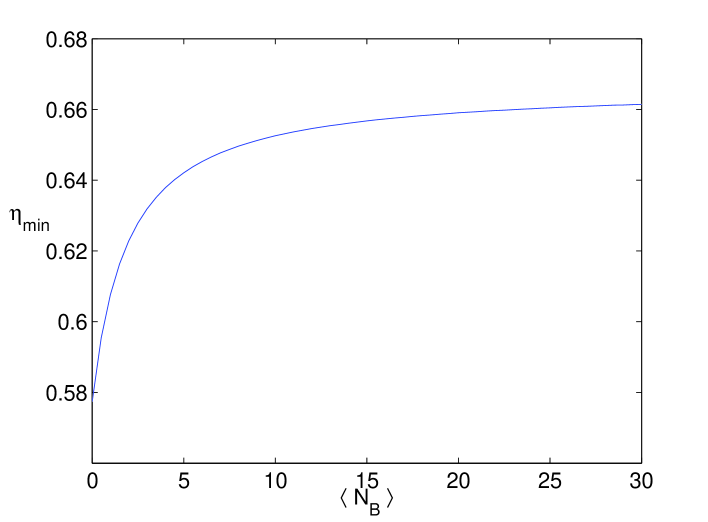
Figure 3.5: Minimum detection efficiency for violation of (3.40) by (3.39) versus mean photon number.

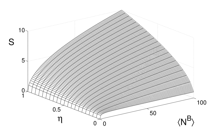
Figure 3.6: Minimum size $S$ of superpositions that may be inferred from violation of (3.44) with the Hamiltonian of (3.39)versus mean photon number.

The existence of macroscopic quantum superpositions [28] are implied by violation of the EPR-Bohm inequality where $\langle N^{B}\rangle$ is large. Measurement of a tiny $\Delta_{est}^{2}j_{z}^{B}$ implies the existence of large superpositions of the eigenstates $|j_{x}^{B}\rangle$ of $J_{x}^{B}$ (or $J_{y}^{B}$), superpositions with a range in $j_{x}^{B}$ of at least

$$S=\sqrt{\langle N^{B}\rangle-2\Delta_{est}^{2}j_{z}^{B}},$$ (3.44)

which becomes $\approx\sqrt{\eta\langle N^{B}\rangle}$ for (3.39) with $\langle N^{B}\rangle$ large (Fig. 3.6). I won’t attempt to explain this point in much detail as it will be the subject of Chapter 5.

Chapter 4 Continuous-Variables Bell inequalities

As we have seen in Chapter 3, Einstein, Podolsky and Rosen (EPR), in their famous 1935 paper [39], demonstrated the incompatibility between the premises of “local realism" and the completeness of quantum mechanics. The original EPR paper used continuous position and momentum variables, and relied on their commutation relations, via the corresponding uncertainty principle. Bohm [14] introduced, in 1951, his version of the EPR paradox with spin observables. This was the version that was used by Bell [7] to prove his famous theorem showing that quantum mechanics predicts results which can rule out the whole class of local hidden variable (LHV) theories. It is hard to overemphasise the importance of this result, which has even been called “the most profound discovery of science” [111]. However, the original Bell inequality, and all of its generalisations, are directly applicable only to the case of discrete observables. The main purpose of this chapter is to close the circle and derive a class of Bell-type inequalities applicable to continuous-variables (CV) correlations, together with multipartite generalisations.

4.1 Motivation

The last decades have witnessed the birth of whole new areas of enquiry, which aim to harness these non-classical correlations predicted by Quantum Mechanics towards information-processing applications. Bell inequality violations have been shown to be relevant for quantum teleportation [90, 56], quantum key distribution [38, 105, 2, 10, 1], and reduction of communication complexity [19]. However there are still many unanswered questions. Bell inequality violation was once thought to be equivalent to entanglement, until Werner [117] showed that there are entangled states that do not violate a large class of Bell inequalities. Gisin [46] proved that all bipartite pure entangled states violate the CHSH [24] inequality, a result which was generalised to the multipartite case by Popescu and Rohrlich [91]. Later, Horodecki et al. [55] devised an analytic criterion to determine whether a mixed state of two qubits have a LHV description. Apart from this simple case, there is no known general method to decide whether a quantum state violates some Bell inequality.

For $n$ parties, $m$ measurements per party and $o$ outcomes, it is well-known that the set of correlations allowed by LHV theories can be represented as a convex polytope, a multi-dimensional geometrical structure formed by all convex combinations (linear combinations where the coefficients are probabilities, i.e., they are non-negative and sum to one) of a finite number of vertices. The vertices of this polytope are the classical pure states — the states with well-defined values for all variables [89, 88, 47]. The tight Bell inequalities are associated with the linear facets of the polytope. It is a computationally hard problem to list all Bell inequalities for given $(n,m,o)$, and full numerical characterisations have been accomplished only for small values of those parameters.

Nevertheless, some special cases can be considered. One can derive classes of Bell inequalities which are recursively defined in terms of those parameters. There are classes for $(n,2,2)$ [78, 5, 12, 124], $(n,3,2)$ [129], $(2,2,o)$ [77, 23] and even $(n,2,o)$ [20, 108], $(n,m,2)$ [128, 73, 81] and $(2,m,o)$ [22]. However, no class of Bell inequalities has previously been derived without any reference to the number $o$ of outcomes or to their bound. Any real experiment will always yield a finite number of outcomes but are there constraints imposed by LHV theories that are independent of any particular discretisation, and can be explicitly written even in the limit $o\rightarrow\infty$? This question goes beyond a challenge proposed in a recent paper by Gisin [47], where he proposes a list of open questions regarding Bell inequalities, which was (in other words) to find inequalities valid for arbitrary but fixed $o$. Our answer is yes; and the derivation is much more straightforward than in the case of the usual Bell-type inequalities which are restricted to a particular set of outputs.

We derive a class of inequalities for local realism that directly uses correlations of measurements, with no restriction to spin measurements or discrete binning. They are not only valid for arbitrary but fixed $o$, but they do not mention the number of outcomes $o$ in their derivation at all. The new inequalities are remarkably simple. They place no restriction on the number of possible outcomes, and the contrast between the classical and quantum bounds involves commutation relations in a central way. They must be satisfied by any observations in a LHV theory, whether having discrete, continuous or unbounded outcomes. We can immediately re-derive previously known Bell-type inequalities, obtaining at the same time their quantum-mechanical bounds by considering the non-commutativity of the observables involved. We also display quantum states that directly violate the new inequalities for continuous, unbounded measurements, even in the macroscopic, large $n$ limit [78, 36, 88, 97]. We show that the new Bell violations survive the effects of finite generation and detection efficiency. This is very surprising, in view of the many examples in which decoherence rapidly destroys macroscopic superpositions [131].

Apart from this intrinsic interest, these inequalities are relevant to an important scientific problem. No experiment has yet produced a Bell inequality violation without introducing either locality or detection loopholes. As emphasised by Gisin in his recent article [47], "quantum nonlocality is so fundamental for our world view that it deserves to be tested in the most convincing way". One path towards this goal is to use continuous-variables and efficient homodyne detection, which allows much higher detection efficiency than is feasible with discrete spin or photo-detection measurements. A number of loop-hole free proposals exist in the literature, but they all use Bell [74, 45, 4, 118, 50] or Hardy [125] inequalities with a dichotomic binning of the results (which usually lead to small violations), or else a parity or pseudo-spin approach [18, 27, 102] which cannot be realized with efficient homodyne detection.

4.2 The variance inequality

We will focus on the correlation functions of observables for $n$ sites or observers, each equipped with $m$ possible apparatus settings to make their causally separated measurements. We consider any real, complex or vector function $F\left(\mathbf{X},\mathbf{Y},\mathbf{Z},\ldots\right)$ of local observations $X_{i},Y_{i},Z_{i}$ at each site $i$, which in an LHV theory are all functions of hidden variables $\lambda$. In a real experiment the different terms in $F$ may not all be measurable at once, because they may involve different choices of incompatible observables. The assumption of locality enters the reasoning by requiring that the local choice of observable does not affect the correlations between variables at different sites, and therefore that the averages are taken over the same hidden variable ensemble $P\left(\lambda\right)$ for all terms. We introduce averages over the LHV ensemble (there’s no loss of generality in considering deterministic LHVs, since, according to Fine’s Theorem 2.8, a phenomenon violates local causality if and only if it violates local determinism [41]),

$$\left\langle F\right\rangle=\int P\left(\lambda\right)F\left(\mathbf{X}\left(\lambda\right),\mathbf{Y}\left(\lambda\right),\mathbf{Z}\left(\lambda\right),\ldots\right)d\lambda.$$ (4.1)

Our LHV inequality uses the simple result that any function of random variables has a non-negative variance,

$$\left|\left\langle F\right\rangle\right|^{2}\leq\langle\left|F\right|^{2}\rangle.$$ (4.2)

We can also give a bound

$$\langle\left|F\right|^{2}\rangle\leq\langle\left|F\right|^{2}\rangle_{sup},$$ (4.3)

where the subscript denotes the supremum (least upper bound), in which products of incompatible observables are replaced by their maximum achievable values. This is necessary since if we are not able to measure both $X_{i}$ and $Y_{i}$ simultaneously, a general LHV model could predict any achievable correlation [112].

The same variance inequality applies to the corresponding Hermitian operator $\hat{F}$ in quantum mechanics. While the observables at different sites commute — they can be simultaneously measured — those at the same site do not, so operator ordering must be included. This enables us to see how quantum theory can violate the variance bound for an LHV.

4.3 An example

As an example, we will apply this variance inequality to a well-known case. Consider two dichotomic observables $X_{i},Y_{i}$ per site $i$, the outcomes of which are $\pm 1$. We define $F_{1}\equiv X_{1}$, $F_{1}^{\prime}\equiv Y_{1}$ , and then inductively construct [44]:

$$F_{n}\equiv\frac{1}{2}(F_{n-1}+F_{n-1}^{\prime})X_{n}+\frac{1}{2}(F_{n-1}-F_{n-1}^{\prime})Y_{n},$$ (4.4)

where $F_{n}^{\prime}$ can be obtained from $F_{n}$ by the exchange $X_{i}\longleftrightarrow Y_{i}$. In calculating $F_{n}^{2}$ we’ll keep track of the local commutators just to make the contrast with quantum mechanics clearer. For real random variables it is obvious that the commutators are zero; at a first read one can just regard that as the act of an overzealous classical theorist. For real variables $X,\,Y$, the commutator is defined in the same way as for the corresponding operators, i.e., $[X,Y]\equiv XY-YX$. The anti-commutator is defined by $[X,Y]_{+}\equiv XY+YX$. Then

$$F_{n}^{2}=\frac{1}{4}\left\{(F_{n-1}^{2}+F_{n-1}^{\prime 2})(X_{n}^{2}+Y_{n}^{2})\right.\\ +[F_{n-1},F_{n-1}^{\prime}]_{+}(X_{n}^{2}-Y_{n}^{2})+(F_{n-1}^{2}-F_{n-1}^{\prime 2})[X_{n},Y_{n}]_{+}\\ \left.-[F_{n-1},F_{n-1}^{\prime}][X_{n},Y_{n}]\right\}.$$ (4.5)

Since $\hat{X}_{n}^{2}=\hat{Y}_{n}^{2}=1$, we can show that $F_{n}^{2}=F_{n}^{\prime 2}$ and

$$F_{n}^{2}=F_{n-1}^{2}-\frac{1}{4}\left[F_{n-1},F_{n-1}^{\prime}\right]\left[X_{n},Y_{n}\right].$$ (4.6)

In a LHV theory, the term which involves commutators will be zero since $[X(\lambda),Y(\lambda)]=X(\lambda)Y(\lambda)-Y(\lambda)X(\lambda)=0$. Hence by induction $F_{n}^{2}=F_{1}^{2}=1$ and the variance inequality (4.2) becomes:

$$-1\leq\left\langle F_{n}\right\rangle\leq 1.$$ (4.7)

This is the Mermin-Ardehali-Belinskii-Klyshko (MABK) [78, 5, 12] Bell inequality, which reduces to the well-known Bell-CHSH [24] inequality for $n=2$.

4.3.1 Quantum bound

We can now calculate the quantum mechanical bound by writing the variance inequality (4.2) and substituting the functions in (4.6) by their corresponding operators

$$\bigl{\langle}\hat{F}_{n}\bigr{\rangle}_{Q}^{2} \leq \bigl{\langle}\hat{F}_{n}^{2}\bigr{\rangle}_{Q}=\bigl{\langle}\hat{F}_{n-1}^{2}-\frac{1}{4}[\hat{F}_{n-1},\hat{F}_{n-1}^{\prime}][\hat{X}_{n},\hat{Y}_{n}]\bigr{\rangle}_{Q}$$ (4.8)

$$\leq \bigl{\|}\hat{F}_{n-1}^{2}\bigr{\|}+\frac{1}{4}\bigl{\|}[\hat{F}_{n-1},\hat{F}_{n-1}^{\prime}]\bigr{\|}\bigl{\|}[\hat{X}_{n},\hat{Y}_{n}]\bigr{\|},$$

where the norm $\left\|A\right\|$ denotes the modulus of the maximum value of $\langle\hat{A}\rangle_{Q}$ over all quantum states. The norm of the second commutator has the bound $\|[\hat{X}_{n},\hat{Y}_{n}]\|\leq 2$. It’s easy to show that $[\hat{F}_{n},\hat{F}_{n}^{\prime}]=\hat{F}_{n-1}^{2}[\hat{X}_{n},\hat{Y}_{n}]+[\hat{F}_{n-1},\hat{F}_{n-1}^{\prime}]$ and therefore $\|[\hat{F}_{n},\hat{F}_{n}^{\prime}]\|\leq 2\|\hat{F}_{n-1}^{2}\|+\|[\hat{F}_{n-1},\hat{F}_{n-1}^{\prime}]\|$ . Solving the recursion relation by noting that $\|\hat{F_{1}^{2}}\|=\frac{1}{2}\|[\hat{X}_{1},\hat{Y}_{1}]\|=1$ we finally arrive at the bound

$$\langle\hat{F_{n}}\rangle_{Q}^{2}\leq 2^{n-1}.$$ (4.9)

This can be attained with the generalised GHZ states [44], which therefore violate (4.2).

4.4 Continuous-variables inequalities

Inspired by those results, we now demonstrate an LHV inequality that is directly applicable to unbounded continuous variables, in particular field quadrature operators. The choice of the function $F_{n}$ in (4.4) is not optimal though, since the variance in general involves incompatible operator products that have no upper bound.

To overcome this problem, consider a complex function $C_{n}$ of the local real observables $\{X_{k},\,Y_{k}\}$ defined as:

$$C_{n}=\tilde{X_{n}}+i\tilde{Y_{n}}=\prod_{k=1}^{n}(X_{k}+iY_{k})\,,$$ (4.10)

so that the modulus square only involves compatible operator products, i.e.

$$\left|C_{n}\right|^{2}=\prod_{k=1}^{n}(X_{k}^{2}+Y_{k}^{2}).$$ (4.11)

Applying the variance inequality to both $\tilde{X_{n}}$ and $\tilde{Y_{n}}$, we find that:

$$\langle\tilde{X}_{n}\rangle^{2}+\langle\tilde{Y_{n}}\rangle^{2}\leq\langle\prod_{k=1}^{n}(X_{k}^{2}+Y_{k}^{2})\rangle$$ (4.12)

This is the main result of this chapter. Given the assumption of local hidden variables, this inequality must be satisfied for any set of observables $X_{k}$, $Y_{k}$, regardless of their spectrum.

4.4.1 Quantum violations

The fact that we have neglected the commutators in deriving (4.12) hints that quantum mechanics might predict a violation. We define quadrature operators

$$\hat{X}_{k} = \hat{a}_{k}e^{-i\theta_{k}}+\hat{a}_{k}^{\dagger}e^{i\theta_{k}}$$

$$\hat{Y}_{k} = \hat{a}_{k}e^{-i(\theta_{k}+s_{k}\pi/2)}+\hat{a}_{k}^{\dagger}e^{i(\theta_{k}+s_{k}\pi/2)},$$ (4.13)

where $\hat{a}_{k},\hat{a}_{k}^{\dagger}$ are the boson annihilation and creation operators at site $k$ and $s_{k}\in\{-1,1\}$.

We now define the operator

$$\hat{Z}_{k}\equiv\hat{X}_{k}+i\hat{Y}_{k}$$ (4.14)

and note that it follows that $\hat{C_{n}}=\prod_{k=1}^{n}\hat{Z}_{k}$. The definition of $\hat{Y}_{k}$ allows for the choice of the relative phase with respect to $\hat{X}_{k}$ to be $\pm\pi/2$. Depending on $s_{k}$, for each $k$ either $\hat{Z}_{k}=2\hat{a}_{k}e^{-i\theta_{k}}$ or $\hat{Z}_{k}=2\hat{a}_{k}^{\dagger}e^{i\theta_{k}}$. Denoting $\hat{A}_{k}(1)=\hat{a}_{k}$ and $\hat{A}_{k}(-1)=\hat{a}_{k}^{\dagger}$, the term in the LHS of (4.12) in quantum mechanics is then

$$|\langle\prod_{k}\hat{Z}_{k}\rangle_{Q}|^{2}=|2^{n}e^{i\sum_{k}s_{k}\theta_{k}}\langle\prod_{k}\hat{A}_{k}(s_{k})\rangle_{Q}|^{2}.$$ (4.15)

The RHS becomes

$$\langle\prod_{k=1}^{n}(X_{k}^{2}+Y_{k}^{2})\rangle_{Q}=\langle\prod_{k=1}^{n}(4\hat{a}_{k}^{\dagger}\hat{a}_{k}+2)\rangle_{Q}$$ (4.16)

regardless of the phase choices. To violate (4.12) we must therefore find a state that satisfies

$$\Bigl{|}\Bigl{\langle}\prod_{k}\hat{A}_{k}(s_{k})\Bigr{\rangle}_{Q}\Bigr{|}^{2}>\Bigl{\langle}\prod_{k}\bigl{(}\hat{a}_{k}^{\dagger}\hat{a}_{k}+\frac{1}{2}\bigr{)}\Bigr{\rangle}_{Q},$$ (4.17)

which is surprisingly insensitive to relative phases between the quadrature measurements at different sites.

This violation of a continuous variable Bell inequality can be realised within quantum mechanics. Consider an even number of sites, choosing $s_{k}=1$ for the first half of them and $s_{k}=-1$ for the remaining. To maximise the LHS we need a superposition of terms which are coupled by that product of annihilation/creation operators. One choice is a state of type

$$\left|\Psi_{S}\right\rangle=c_{0}\left|0,\dots,0,1,\dots,1\right\rangle+c_{1}\left|1,\dots,1,0,\dots,0\right\rangle,$$ (4.18)

where in the first term the first $n/2$ modes are occupied by zero photons and the remaining by $1$; conversely for the second term. With that choice of state the LHS of (4.17) becomes $|c_{0}|{{}^{2}}|c_{1}|{{}^{2}}$, which is maximised by $|c_{0}|^{2}=|c_{1}|^{2}=\frac{1}{2}$. The RHS is $(\frac{3}{2})^{\frac{n}{2}}(\frac{1}{2})^{\frac{n}{2}}$ independently of the amplitudes $c_{0},\,c_{1}$. Dividing the LHS by the RHS, inequality (4.17) becomes $\frac{1}{4}\left(\frac{4}{3}\right)^{\frac{n}{2}}\leq 1$, which is violated for $n\geq 10$, and the violation grows exponentially with the number of sites.

4.4.2 Feasibility

While setting up the homodyne detectors necessary for this observation is challenging, the complexity of this task scales linearly with the number of modes. A more stringent constraint is most likely in the state preparation, but we can relate state (4.18) to a class of states of great experimental interest. They can be achieved from a generalised GHZ state of $n/2$ photons,

$$|GHZ(n)\rangle=\frac{1}{\sqrt{2}}(|H\rangle^{\otimes\frac{n}{2}}+|V\rangle^{\otimes\frac{n}{2}}),$$ (4.19)

where $|H\rangle$ and $|V\rangle$ respectively represent single-particle states of horizontal and vertical polarisation — by splitting each mode with a polarising beam splitter. Therefore violation of (4.12) can be observed in the ideal case with a 5-qubit photon polarisation GHZ state and homodyne detection.

An interesting question is the effect of decoherence, both from state preparation error [60] and detector inefficiency. The usual Bell-CHSH violations have an efficiency threshold [49] of $83\%$. This has not yet been achieved for single-photon counting. Homodyne detection is remarkably efficient by comparison ([75] report up to 94.4%, for example). However, the effect of detector efficiency is easily included by assuming that each detected photon mode is preceded by a beam splitter with intensity transmission $\eta<1$. This changes both the LHS and RHS, so that the inequality becomes $\frac{4\eta^{2}}{2\eta+1}\leq 4^{2/n}$, giving a threshold efficiency requirement of $\eta>\eta_{min}$, where

$$\eta_{min}=(1+\sqrt{1+4^{1-2/n}})/4^{1-2/n}.$$ (4.20)

This reduces at large $n$ to an asymptotic value of $\eta_{\infty}=0.80902$. Unexpectedly, the Bell violation (which signifies a quantum superposition) is less sensitive to detector inefficiency in the macroscopic, large $n$ limit. The minimum detector efficiency $\eta_{n}$ at finite $n$ is plotted in Fig. 1, together with the minimum state preparation fidelity $\epsilon_{min}$ in the case of ideal detectors, where we model the density matrix as

$$\hat{\rho}=\epsilon|\Psi_{S}\rangle\langle\Psi_{S}|+(1-\epsilon)\hat{I}.$$ (4.21)

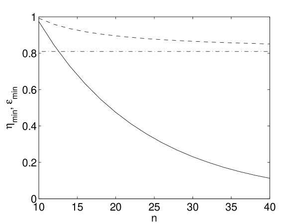
Figure 4.1: Minimum state preparation fidelity $\epsilon_{min}$ for ideal detectors (solid line), and minimum detection efficiency $\eta_{min}$ for ideal state preparation (dashed line) required for violation of (4.12) as a function of the number of modes. The asymptotic value of $\eta_{min}$ is indicated by the dash-dotted line.

4.5 No-go proof for first-moment correlation C.V. Bell inequalities

We will finally prove that there are no LHV inequalities possible if one considers only the first-moment correlations between continuous variables in different sites. We will show this explicitly for the simplest case and indicate how to generalise to arbitrary numbers of parties and settings. Consider first $n=2$ parties, Alice and Bob, each of which can choose between $m=2$ observables: $X_{a},Y_{a}$ for Alice and $X_{b},Y_{b}$ for Bob. Each measurement yields an outcome in the real numbers. The first-moment correlation functions for each of the $4$ possible configurations are just the averages $\langle X_{a}X_{b}\rangle$, $\langle X_{a}Y_{b}\rangle$, $\langle Y_{a}X_{b}\rangle$, $\langle Y_{a}Y_{b}\rangle$. Given those $4$ experimental outcomes, can we find a local hidden variable model which reproduces them?

We construct an explicit example. Consider a hidden-variable state $S$ where the hidden variables are the measured values $\mathbf{X},\,\mathbf{Y}$, in an equal mixture of four classical pure states $S_{k}=\left(X_{a},Y_{a},X_{b},Y_{b}\right)_{k}$ defined by

$$\begin{split}S_{1}&=2\,(1,0,\langle X_{a}X_{b}\rangle,0)\\ S_{2}&=2\,(1,0,0,\langle X_{a}Y_{b}\rangle)\\ S_{3}&=2\,(0,1,\langle Y_{a}X_{b}\rangle,0)\\ S_{4}&=2\,(0,1,0,\langle Y_{a}Y_{b}\rangle).\end{split}$$ (4.22)

Each of the states $S_{k}$ assigns a nonzero value to only one of the $4$ correlation functions. Since the probability of each of the states in the equal mixture is $1/4$, we have for example $\langle X_{a}X_{b}\rangle_{S}=\frac{1}{4}\sum_{i}\langle X_{a}X_{b}\rangle_{S_{i}}=\langle X_{a}X_{b}\rangle$.

Satisfying the two-site correlations using the state $S$ defined by (4.22) leaves us with uncontrolled values for the single-site correlations, for instance $\langle X_{b}\rangle_{S}=\frac{1}{2}(\langle X_{a}X_{b}\rangle+\langle Y_{a}X_{b}\rangle)$. One might object to the fact that this is not equal to $\langle X_{b}\rangle$ in general. However, we may correct these lower order correlations by adding four more states ($S_{5}$ to $S_{8}$) and changing the prefactors multiplying $S_{1}$ to $S_{4}$ to compensate for their reduced weight in the equal mixture. Crucially, adding these extra states to $S$ in this manner does not modify the values of correlations such as $\langle X_{a}X_{b}\rangle$. As an example, we exhibit the state

$$S_{5}=8\,(0,0,\langle X_{b}\rangle-(\langle X_{a}X_{b}\rangle+\langle Y_{a}X_{b}\rangle)/\sqrt{8},0),$$ (4.23)

which corrects the single expectation value $\langle X_{b}\rangle_{S}$ to $\langle X_{b}\rangle$.

The proof generalises easily to arbitrary $n$ and $m$. In that case, there are $m^{n}$ possible combinations of measurements which yield $n$-site correlations. Denoting the $j^{\mathrm{th}}$ observable at site $i$ by $X_{i}^{j}$, each combination is specified by a sequence of indices $(j_{1},j_{2},\dotsc,j_{n})$. For each combination of measurements, we define a hidden variable state which assigns nonzero values only to the variables which appear in the associated correlation function $\langle\prod_{i=1}^{n}X_{i}^{j_{i}}\rangle$. In analogy to the example above, we can always choose the values of the hidden variables associated to $X_{i}^{j_{i}}$ such that their product is equal to $m^{n}\langle\prod_{i=1}^{n}X_{i}^{j_{i}}\rangle$. Since all other $m^{n}-1$ states defined in this way will give a value of zero to this particular correlation function, and given that the probability associated with each of those states is $1/m^{n}$, we reproduce all correlations as desired. As indicated in the example, additional first moment correlations involving less than $n$ sites can be included in the LHV model by adding additional states to $S$ in a way which doesn’t affect the $n$-site correlations. Thus, any possible observation of first moment correlations may be explained using a LHV model, and hence these correlations alone cannot violate any Bell inequality. In other words, the minimum requirement for a correlation Bell inequality with continuous, unbounded variables, is to use not just the first but also the second moments at each site.

4.6 Concluding remarks

In conclusion, in this chapter we have derived a new class of Bell-type inequalities valid for continuous and unbounded experimental outcomes. We have shown that the same procedure allows one to derive the MABK class of Bell inequalities and their corresponding quantum bounds. That derivation makes it explicit that non-zero commutators — associated with the incompatibility of the local observables — are the essential ingredient responsible for the discrepancy between quantum mechanics and local hidden variable theories. The new Bell-type inequality derived here can be directly applied to continuous variables without the need for a specific binning of the measurement outcomes. Surprisingly, quantum mechanics predicts exponentially increasing violations of the inequality for macroscopically large numbers of sites, even including realistic decoherence effects like inefficient state preparation, and a detector loss at every site.

Chapter 5 Generalised Macroscopic Superpositions

5.1 Introduction

Since Schrödinger’s seminal essay of 1935 [104], in which he introduced his famous cat paradox, there has been a great deal of interest and debate on the subject of the existence of a superposition of two macroscopically distinguishable states. This issue is closely related to the so-called measurement problem [130]. Some attempts to solve this problem, such as that of Ghirardi, Rimini, Weber and Pearle [52, 51], introduce modified dynamics that cause a collapse of the wave function, effectively limiting the size of allowed superpositions.

It thus becomes relevant to determine whether a superposition of states with a certain level of distinguishability can exist experimentally [80]. Evidence [11, 9, 42, 93, 79, 3, 34, 85] for quantum superpositions of two distinguishable states has been put forward for a range of different physical systems including SQUIDs, trapped ions, optical photons and photons in microwave high-Q cavities. Signatures for the size of superpositions have been discussed by Leggett [70] and, more recently, by Korsbakken et al [63]. Theoretical work suggests that the generation of a superposition of two truly macroscopically distinct states will be greatly hindered by decoherence [25, 131].

In a recent paper [28], we suggested to broaden the concept of detection of macroscopic superpositions, by focusing on signatures that confirm, for some experimental instance, a failure of microscopic/mesoscopic superpositions to predict the measured statistics. This approach is applicable to a broader range of experimental situations based on macroscopic systems, where there would be a macroscopic range of outcomes for some observable, but not necessarily just two that are macroscopically distinct. Recent work by Marquardt et al [75] reports experimental application of this approach.

The paradigmatic example [69, 71, 9, 79, 42, 93, 11, 3, 34, 85] of a macroscopic superposition involves two states $\psi_{+}$ and $\psi_{-}$, macroscopically distinct in the sense that the respective outcomes of a measurement $\hat{x}$ fall into regions of outcome domain, denoted $+$ and $-$, that are macroscopically different. We argue in [28] that a superposition of type

$$\psi_{+}+\psi_{0}+\psi_{-},$$ (5.1)

that involves a range of states but with only some pairs (in this case $\psi_{+}$and $\psi_{-}$) macroscopically distinct must also be considered a type of macroscopic superposition (we call these generalised macroscopic superpositions), in the sense that it displays a nonzero off-diagonal density matrix element $\langle\psi_{+}|\rho|\psi_{-}\rangle$, connecting two macroscopically distinct states, and hence cannot be constructed from microscopic superpositions of the basis states of $\hat{x}$. Such superpositions [77, 36, 87, 99] are predicted to be generated in certain key macroscopic experiments, that have confirmed continuous-variable [84, 132, 109, 16, 110, 17, 62, 61, 68, 21, 114] squeezing and entanglement, spin squeezing and entanglement of atomic ensembles [64, 65], and entanglement and violations of Bell inequalities for discrete measurements on multi-photon systems [33, 67, 101, 72].

We derive criteria for the detection of the generalised macroscopic (or $S$-scopic) superpositions using continuous variable measurements. These criteria confirm that a macroscopic system cannot be described as any mixture of only microscopic (or $s$-scopic, where $s<S$) quantum superpositions of eigenstates of $\hat{x}$. We show how to apply the criteria to detect generalised $S$-scopic superpositions in squeezed and entangled states that are of experimental interest.

The generalised macroscopic superpositions still hold interest from the point of view of Schrödinger’s discussion [104] of the apparent incompatibility of quantum mechanics with macroscopic realism. This is so because such superpositions cannot be represented as a mixture of states which give outcomes for $\hat{x}$ that always correspond to one or other (or neither) of the macroscopically distinct regions $+$ and $-$. The quantum mechanical paradoxes associated with the generalised macroscopic superposition (5.1) have been discussed in previous works [28, 77, 36, 94, 29].

The criteria derived in this chapter take the form of inequalities. Their derivation utilises the uncertainty principle and the assumption of certain types of mixtures. In this respect they are similar to criteria for inseparability that have been derived by Duan et al. and Simon [32, 107] and Hofmann and Takeuchi [58]. Rather than testing for failure of separable states, however, they test for failure of a phase space “macroscopic separability”, where it is assumed that a system is always in a mixture (never a superposition) of macroscopically separated states.

We will note that one can be more general in the derivation of the inequalities, adopting the approach of Leggett and Garg [71] to define a macroscopic reality without reference to any quantum concepts. One may consider a whole class of theories, which we refer to as the minimum uncertainty theories (MUT) and to which quantum mechanics belongs, for which the uncertainty relations hold and the inequalities therefore follow, based on this macroscopic reality. The experimental confirmation of violation of these inequalities will then lead to demonstration of a new type of Einstein-Podolsky-Rosen argument (or “paradox”) [39], in which the inconsistency of a type of macroscopic ($S$-scopic) reality with the completeness of quantum mechanics is revealed [28, 94]. A direct analogy exists with the original EPR argument, which is a demonstration of the incompatibility of local realism with the completeness of quantum mechanics [98, 120, 95]. In our case, the inconsistency of the completeness of quantum mechanics is shown to be with a macroscopic reality rather than the local reality of the original EPR argument.

5.2 Generalised $S$-scopic Coherence

We introduce in this Section the concept of a generalised $S$-scopic coherence [28], which we define in terms of failure of certain types of mixtures. In the next Section, we link this concept to that of the generalised $S$-scopic superpositions (5.1).

We consider a system which is in a statistical mixture of two component states. For example, if one attributes probabilities $\wp_{1}$ and $\wp_{2}$ to underlying quantum states $\rho_{1}$ and $\rho_{2}$, respectively (where $\rho_{i}$ denotes a quantum density operator), then the state of the system will be described as a mixture, which in quantum mechanics is represented as

$$\rho=\wp_{1}\rho_{1}+\wp_{2}\rho_{2}.$$ (5.2)

This can be interpreted as "the state is either $\rho_{1}$ with probability $\wp_{1}$, or $\rho_{2}$ with probability $\wp_{2}$". The probability for an outcome $x$ of any measurable physical quantity $\hat{x}$ can be written, for a mixture of the type (5.2), as

$$P(x)=\wp_{1}P_{1}(x)+\wp_{2}P_{2}(x),$$ (5.3)

where $P_{i}(x)$ ($i=1,2$) is the probability distribution of $x$ in the state $\rho_{i}$.

More generally, in any physical theory, the specification of a state $\rho$ (where here $\rho$ is just a symbol to denote the state, but not necessarily a density matrix) fully specifies the probabilities of outcomes of all experiments that can be performed on the system. If we then have with probability $\wp_{1}$ a state $\rho_{1}$ which predicts for each observable $\hat{x}$ a probability distribution $P_{1}(x)$ and with probability $\wp_{2}$ a second state which predicts $P_{2}(x)$, then the probability distribution for any observable $\hat{x}$ given such mixture is of the form (5.3).

The concept of coherence can now be introduced.

Definition 1: The state of a physical system displays coherence between two outcomes $x_{1}$ and $x_{2}$ of an observable $\hat{x}$ iff the state $\rho$ of the system cannot be considered a statistical mixture of some underlying states $\rho_{1}$ and $\rho_{2}$, where $\rho_{1}$ assigns probability zero for $x_{2}$ and $\rho_{2}$ assigns probability zero for $x_{1}$.

This definition is independent of quantum mechanics. Within quantum mechanics it implies that the quantum density matrix representing the system cannot be decomposed in the form (5.2). Thus, for example, $\rho=\frac{1}{\sqrt{2}}(|\psi_{+}\rangle\langle\psi_{+}|+|\psi_{-}\rangle\langle\psi_{-}|),$ where $|\psi_{\pm}\rangle=[|x_{1}\rangle\pm|x_{2}\rangle]/\sqrt{2},$ does not display coherence between $x_{1}$ and $x_{2}$ because it can be rewritten to satisfy (5.2). The definition will allow a state to be said to have coherence between $x_{1}$ and $x_{2}$ if and only if there is no possible ensemble decomposition of that state which allows an interpretation as a mixture (5.2), so that the system cannot be regarded as being in one or other of the states that can generate at most one of $x_{1}$ or $x_{2}$.

We next define the concept of generalised $S$-scopic coherence.

Definition 2: We say that the state displays generalised $S$-scopic coherence iff there exist $x_{1}$ and $x_{2}$ with $x_{2}-x_{1}\geq S$ (we take $x_{2}>x_{1}$), such that $\rho$ displays coherence between outcomes $x\leq x_{1}$ and $x\geq x_{2}$. This coherence will be said to be macroscopic when $S$ is macroscopic.

If there is no generalised $S$-scopic coherence, then the system can be described as a mixture (5.2) where now states $\rho_{1}$ and $\rho_{2}$ assign nonzero probability only for $x<x_{2}$ and $x>x_{1}$ respectively. This situation is depicted in Fig. 5.1.

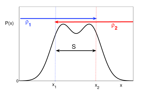
Figure 5.1: Probability distribution for outcomes $x$ of measurement $\hat{x}$. If $x_{1}$ and $x_{2}$ are macroscopically separated, then we might expect the system to be described as the mixture (5.2), where $\rho_{1}$ encompasses outcomes $x<x_{2}$, and $\rho_{2}$ encompasses outcomes $x>x_{1}$. This means an absence of generalised macroscopic coherence, as defined in Section 5.2.

An important clarification is needed at this point. It is clearly a vague matter to determine when $S$ is macroscopic. What is important is that we are able to push the boundaries of experimental demonstrations of $S$-scopic coherence to larger values of $S$. We will keep the simpler terminology, but the reader might want to understand macroscopic as $S$-scopic throughout the text.

Generalised macroscopic coherence amounts to a loss of what we will call a generalised macroscopic reality. The simpler form of macroscopic reality that involves only two states macroscopically distinct has been discussed extensively by Leggett [69, 71]. This simpler case would be applicable to the situation of Fig. 1 if there were zero probability for result in the intermediate region $x_{1}<x<x_{2}$. Macroscopic reality in this simpler situation means that the system must be in one or other of two macroscopically distinct states, $\rho_{1}$ and $\rho_{2}$, that predict outcomes in regions $x\leq x_{1}$ and $x\geq x_{2}$, respectively. The term “macroscopic reality” is used [71] because the definition precludes that the system can be in a superposition of two macroscopically distinct states prior to measurement. Generalised macroscopic reality applies to the broader situation, where probabilities for outcomes $x_{1}<x<x_{2}$ are not zero, and means that where we have two macroscopically separated outcomes $x_{1}$ and $x_{2}$, the system can be interpreted as being in one or other of two states $\rho_{1}$ and $\rho_{2}$, that can predict at most one of $x_{1}$ or $x_{2}$. Again, the term macroscopic reality is used, because this definition precludes that the system is a superposition of two macroscopically separated states that give outcomes $x_{1}$ and $x_{2}$ respectively.

We note that Leggett and Garg [71] define a macroscopic reality in which they do not restrict to quantum states $\rho_{1}$ and $\rho_{2}$, but allow for a more general class of theories where $\rho_{1}$ and $\rho_{2}$ can be hidden variable states of the type considered by Bell [7]. Such states are not restricted by the uncertainty relation that would apply to each quantum state, and hence the assumption of macroscopic reality as applied to these theories would not lead to the inequalities we derive in this chapter. This point will be discussed in Section 5.4, but the reader should note the definition of $S$-scopic coherence within quantum mechanics means that $\rho_{1}$ and $\rho_{2}$ are quantum states.

5.3 Generalised macroscopic and $S$-scopic quantum Superpositions

We now link the definition of generalised macroscopic coherence to the definition of generalised macroscopic superposition states [28]. Generally we can express $\rho$ as a mixture of pure states $|\psi_{i}\rangle$. Thus

$$\rho=\sum_{i}\wp_{i}|\psi_{i}\rangle\langle\psi_{i}|,$$ (5.4)

where we can expand each $|\psi_{i}\rangle$ in terms of a basis set such as the eigenstates $|x\rangle$ of $\hat{x}$: thus $|\psi_{i}\rangle=\sum_{x}c_{x}|x\rangle$, the $c_{x}$ being probability amplitudes.

Theorem A: The existence of coherence between outcomes $x_{1}$ and $x_{2}$ of an observable $\hat{x}$ is equivalent, within quantum mechanics, to the existence of a nonzero off-diagonal element in the density matrix, i.e, $\left\langle x_{1}\right|\rho\left|x_{2}\right\rangle\neq 0$.

Proof: The proof is given in Appendix A. $\blacksquare$

Theorem B: In quantum mechanics, there exists coherence between outcomes $x_{1}$ and $x_{2}$ of an observable $\hat{x}$ iff in any decomposition (B.1) of the density matrix, there is a nonzero contribution from a superposition state of the type

$$|\psi_{S}\rangle=c_{x_{1}}\left|x_{1}\right\rangle+c_{x_{2}}\left|x_{2}\right\rangle+\sum_{x\neq x_{1},x_{2}}c_{x}\left|x\right\rangle$$ (5.5)

with $c_{x_{1}}$,$c_{x_{2}}\neq 0$.

Proof: If each $|\psi_{i}\rangle$ cannot be written in the specific form (5.5), then each $|\psi_{i}\rangle\langle\psi_{i}|$ is either of form $\rho_{1}$ or $\rho_{2}$, so that we can write $\rho$ as the mixture (5.2). Hence the existence of coherence, which implies $\rho$ cannot be written as (5.2), implies the superposition must always exist in (B.1). The converse is also true: if the superposition exists in any decomposition, then there exists an irreducible term in the decomposition that assigns nonzero probabilities to both $x_{1}$ and $x_{2}$, and therefore the density matrix cannot be written as (5.2). $\blacksquare$

We say that a generalised $S$-scopic superposition of states $|x_{1}\rangle$ and $|x_{2}\rangle$ exists when any decomposition (B.1) must contain a nonzero probability for a superposition (5.5), where $x_{1}$ and $x_{2}$ are separated by at least $S$. Throughout this chapter, we define the size $S$ of the generalised superposition

$$|\psi\rangle=\sum_{k}c_{k}|x_{k}\rangle$$ (5.6)

(where $|x_{k}\rangle$ are eigenstates of $\hat{x}$ and each $c_{k}\neq 0$) to be the range of its prediction for $\hat{x}$, this range being the maximum value of $|x_{k}-x_{j}|$ where $|x_{k}\rangle$ and $|x_{j}\rangle$ are any two components of the superposition (5.6) (so $c_{k}$,$c_{j}\neq 0$).

From the above discussions it follows that within quantum mechanics, the existence of generalised $S$-scopic coherence between $x_{1}$ and $x_{2}$ (here $|x_{2}-x_{1}|=S$) implies the existence of a generalised $S$-scopic superposition of type (5.5), which can be written as

$$|\psi\rangle=c_{-}\psi_{-}+c_{0}\psi_{0}+c_{+}\psi_{+},$$ (5.7)

where the quantum state $\psi_{-}$ assigns some nonzero probability only to outcomes smaller than or equal to $x_{1}$, the quantum state $\psi_{+}$ assigns some nonzero probability only to outcomes larger than or equal to $x_{2}$, and the state $\psi_{0}$ assigns nonzero probabilities only to intermediate values satisfying $x_{1}<x<x_{2}$. Where $S$ is macroscopic, expression (5.7) depicts a generalised macroscopic superposition state. In this case then, only the states $\psi_{-}$ and $\psi_{+}$ are necessarily macroscopically distinct. We regain the traditional extreme macroscopic quantum state $c_{-}\psi_{-}+c_{+}\psi_{+}$ when $c_{0}=0$.

5.4 Minimum Uncertainty Theories

We now follow a procedure similar to that used to derive criteria useful for the confirmation of inseparability [32]. The underlying states $\rho_{1}$ and $\rho_{2}$ comprising the mixture (5.2) are themselves quantum states, and so each will satisfy the quantum uncertainty relations with respect to complementary observables. This and the assumption of (5.2) will imply a set of constraints. The violation of any one of these is enough to confirm the observation of a generalised macroscopic coherence- that is, of a generalised macroscopic superposition of type (5.7).

While our specific aim is to develop criteria for quantum macroscopic superpositions, we present the derivations in as general a form as possible to make the point that experimental violation of the inequalities would imply not only a generalised macroscopic coherence in quantum theory, but a failure of the assumption (5.3) in all theories which place the system in a probabilistic mixture of two states, which we designate by $\rho_{1}$ and $\rho_{2}$, and for which the appropriate uncertainty relation holds for each of the states. In this sense, our approach is similar to that of Bell [7], except that the assumption used here of minimum uncertainties for outcomes of measurements would be regarded as more restrictive than the general hidden variable theories considered by Bell.

We make this point more specific by defining a whole class of theories, which we refer to as the Minimum Uncertainty Theories (MUT), that embody the assumption that any state $\rho$ within the theory will predict the same uncertainty relation for the variances of two incompatible observables $\hat{x}$ and $\hat{p}$ as is predicted by quantum mechanics. This is a priori not an unreasonable thing to postulate for a theory that may differ from quantum mechanics in the macroscopic regime but agree with all the observations in the well-studied microscopic regime. Here we will focus on pairs of observables, like position and momentum, for which the uncertainty bound is a real number, which with the use of scaling and choice of units will be set to $1$, so we can write the an uncertainty relation assumed by all MUT’s as

$$\Delta^{2}x\Delta^{2}p\geq 1,$$ (5.8)

where $\Delta^{2}x$ and $\Delta^{2}p$ are the variances of $x$ and $p$ respectively. This is Heisenberg’s uncertainty relation, and quantum mechanics is clearly a member of MUT. Other quantum uncertainty relations that will be specifically used in this chapter include

$$\Delta^{2}x+\Delta^{2}p\geq 2,$$ (5.9)

which follows from (5.8) and has been useful in derivation of inseparability criteria [32].

5.5 Signatures for generalised S-scopic superpositions: Binned domain

In this Section we will derive inequalities that follow if there are no $s$-scopic superpositions (where $s>S$), so that violation of these inequalities implies existence of an $S$-scopic superposition (or coherence), as defined in Sections 5.2 and 5.3. The approach is similar to that often used to detect entangled states. Separability implies inequalities such as those derived by Duan et al. and Simon [32, 107], and their violation thus implies existence of entanglement. This approach has been used to experimentally confirm entanglement, as described in reference [17], among others. An experimental description of the approach we use here has also been outlined by Marquardt et al. [75].

We consider two types of criteria for the detection of a generalised macroscopic superposition (or coherence). The first, of the type considered in [28], will be considered in this section and uses binned outcomes to demonstrate a generalised $S$-scopic superposition of states $\psi_{+}$ and $\psi_{-}$ that predict outcomes in specified regions denoted $+1$ and $-1$ respectively (Fig. 2), where these regions are separated by a minimum distance $S$. We expand on some earlier results of [28] for completeness and also introduce new criteria of this type.

5.5.1 Single system

Consider a system $A$ and a macroscopic measurement $\hat{x}$ on $A$, the outcomes of which are spread over a macroscopic range. We partition the domain of outcomes $x$ for this measurement into three regions, labelled $l=-1,0,1$ for the regions $x\leq-S/2$, $-S/2<x<S/2$, $x\geq S/2$, respectively. The probabilities for outcomes to fall in those regions are denoted $\wp_{-},$ $\wp_{0}$ and $\wp_{+}$, respectively (Fig. 2).

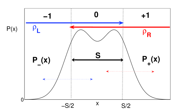
Figure 5.2: Probability distribution for a measurement $\hat{x}$ . We bin results to give three distinct regions of outcome: $0$, $-1,$$+1$.

If there is no generalised S-scopic coherence then there is no coherence between outcomes in $l=1$ and $l=-1$, and the state of system $A$ can be written as

$$\rho_{mix}=\wp_{L}\rho_{L}+\wp_{R}\rho_{R},$$ (5.10)

where $\rho_{L}$ predicts outcomes in the region $x<S/2$, $\rho_{R}$ predicts outcomes in the region $x>-S/2$, and $\wp_{L}$ and $\wp_{R}$ are their respective probabilities. The assumption of this mixture (5.10) implies

$$P(y)=\wp_{L}P_{L}(y)+\wp_{R}P_{R}(y).$$ (5.11)

Here $y$ is the outcome of some measurement that can be performed on the system, and $P_{R/L}(y)$ is the probability for a result $y$ when the system is specified as being in state $\rho_{R/L}$. Where the measurement performed is $\hat{x}$, so $y=x$, there is the constraint on (5.11) so that $P_{R}(x)=0$ for $x\leq-S/2$ and $P_{L}(x)=0$ for $x\geq S/2$.

Now consider an observable $\hat{p}$ (with outcomes $p$) incompatible with $\hat{x}$, such that the variances are constrained by the uncertainty relation $\Delta^{2}x\Delta^{2}p\geq 1$. Our goal is to derive inequalities from just two assumptions: firstly, that $\hat{x}$ and $\hat{p}$ are incompatible observables of quantum mechanics (or of a Minimum Uncertainty Theory), so the uncertainty relation holds for both $\rho_{R/L}$; and, secondly, that there is no generalised S-scopic coherence.

Violation of these inequalities will imply that one of these assumptions is false. Within quantum mechanics, for which the first assumption is necessarily true, that would imply the existence of a generalised macroscopic superposition of type (5.7) with outcomes $x_{1}$ and $x_{2}$ separated by at least $S$.

If the quantum state is of form (5.10) or if the theory satisfies (5.11), then

$$\Delta^{2}p\geq\wp_{L}\Delta_{L}^{2}p+\wp_{R}\Delta_{R}^{2}p,$$ (5.12)

where $\Delta{{}^{2}}p$, $\Delta{{}^{2}}_{L}p$ and $\Delta{{}^{2}}_{R}p$ are the variances of $p$ in the states $\rho_{mix}$, $\rho_{L}$ and $\rho_{R}$, respectively. This follows simply from the fact the variance of a mixture cannot be less than the average variance of its component states. Specifically, if a probability distribution for a variable $z$ is of the form $P(z)=\sum_{i=1}^{N}\wp_{i}P(z)$, then $\Delta^{2}z=\sum_{i=1}^{N}\wp_{i}\Delta_{i}^{2}z+\frac{1}{2}\sum_{i\neq i^{\prime}}\wp_{i}\wp_{i^{\prime}}(\langle z\rangle_{i}-\langle z\rangle_{i^{\prime}})^{2}$.

We can now, using (5.12) and the Cauchy-Schwarz inequality, derive a bound for a particular function of variances that will apply if the system is describable as (5.10)

$$(\wp_{L}\Delta_{L}^{2}x+\wp_{R}\Delta_{R}^{2}x)\Delta^{2}p \geq [\sum_{i=L,R}\wp_{i}\Delta_{i}^{2}x][\sum_{i=L,R}\wp_{i}\Delta_{i}^{2}p]$$

$$\geq [\sum_{i=L,R}\wp_{i}\Delta_{i}x\Delta_{i}p]^{2}$$

$$\geq 1.$$

The left hand side is not directly measurable, since it involves variances of $\hat{x}$ in two states which have overlapping ranges of outcomes. We must derive an upper bound for $\Delta_{L/R}^{2}x$ in terms of measurable quantities. For this we partition the probability distribution $P_{R}(x)$ according to the outcome domains $l=0,1$, into normalised probability distributions $P_{R0}(x)\equiv P_{R}(x|x<S/2)$, and $P_{+}(x)\equiv P_{R}(x|x\geq S/2)$:

$$P_{R}(x)=\wp_{R0}P_{R0}(x)+\wp_{R+}P_{+}(x).$$ (5.14)

Here $\wp_{R+}=\int_{S/2}^{\infty}P_{R}(x)dx=\wp_{+}$ and $\wp_{R0}=\int_{0}^{S/2}P_{R}(x)dx$. It follows that $\Delta_{R}^{2}x=\wp_{R0}\Delta_{R0}^{2}x+\wp_{R+}\Delta_{+}^{2}x+\wp_{R0}\wp_{R+}(\mu_{+}-\mu_{R0})^{2}$, where $\mu_{+}$($\Delta_{+}^{2}x$) and $\mu_{R0}$ ($\Delta_{R0}^{2}x$) are the averages (variances) of $P_{+}(x)$ and $P_{R0}(x)$, respectively. Using the bounds $\wp_{R0}\leq\wp_{0}/(\wp_{0}+\wp_{+})$, $\Delta_{R0}^{2}x\leq S^{2}/4$, $\wp_{R+}\leq 1$ and $0\leq\mu_{+}-\mu_{R0}\leq\mu_{+}+S/2$, we derive

$$\Delta_{R}^{2}x\leq\Delta_{+}^{2}x+\frac{\wp_{0}}{\wp_{0}+\wp_{+}}[(S/2)^{2}+(\mu_{+}+S/2)^{2}]$$ (5.15)

and, by similar reasoning,

$$\Delta_{L}^{2}x\leq\Delta_{-}^{2}x+\frac{\wp_{0}}{\wp_{0}+\wp_{-}}[(S/2)^{2}+(\mu_{-}-S/2)^{2}].$$ (5.16)

Here $\mu_{\pm}$ and $\Delta_{\pm}^{2}x$ are the mean and variance of the measurable $P_{\pm}(x)$, which, since the only contributions to the regions + and - are from $P_{R}(x)$ and $P_{L}(x)$ respectively, are defined as the normalised $+$ and $-$ parts of $P(x)$, so that $P_{+}(x)\equiv P(x|x\geq S/2)$ and $P_{-}(x)\equiv P(x|x\leq-S/2)$. We substitute (5.15) in (5.5.1), and use $\wp_{0}+\wp_{+}\geq\wp_{R}$ and $\wp_{0}+\wp_{-}\geq\wp_{L}$ to derive the final result which is expressed in the following theorem.

Theorem 1: The assumption of no generalised $S$-scopic coherence between outcomes in regions $+1$ and $-1$ of Fig. 2 (or, equivalently, of no generalised $S$-scopic superpositions involving two states $\psi_{-}$ and $\psi_{+}$ predicting outcomes for $\hat{x}$ in the respective regions $+1$ and $-1$) will imply the uncertainty relations

$$(\Delta_{ave}^{2}x+\wp_{0}\delta)\Delta^{2}p\geq 1$$ (5.17)

and

$$\Delta_{ave}^{2}x+\Delta^{2}p\geq 2-\wp_{0}\delta,$$ (5.18)

where we define $\Delta_{ave}^{2}x=\wp_{+}\Delta_{+}^{2}x+\wp_{-}\Delta_{-}^{2}x$ and $\delta\equiv\{(\mu_{+}+S/2)^{2}+(\mu_{-}-S/2)^{2}+S{{}^{2}}/2\}+\Delta_{+}^{2}x+\Delta_{-}^{2}x$. Thus, the violation of either one of these inequalities implies the existence of a generalised $S$-scopic quantum superposition, and in this case the superposition involves states $\psi_{+}$ and $\psi_{-}$ predicting outcomes for $\hat{x}$ in regions $+1$ and $-1$, of Fig. 2, respectively.).

As illustrated in Fig.2, the $\Delta_{\pm}^{2}x$ and $\mu_{\pm}$ are the variance and mean of $P_{\pm}(x)$, the normalised distribution over the domain $l=\pm 1$. $\wp_{\pm}$ is the total probability for a result $x$ in the domain $l=\pm 1$, while $\wp_{0}=1-(\wp_{+}+\wp_{-})$. The measurement of the probability distributions for $\hat{x}$ and $\hat{p}$ are all that is required to determine whether violation of the inequality (5.17) or (5.18) occurs. Where $\hat{x}$ and $\hat{p}$ correspond to optical field quadratures, such distributions have been measured, for example, by Smithey et al [103].

Proof: The assumption of no such generalised $S$-scopic superposition implies (5.10). We have proved that (5.17) follows. To prove (5.18), we start from (5.10) and the uncertainty relation (5.9), and derive a bound that will apply if the system is describable as (5.10): $(\wp_{L}\Delta_{L}^{2}x+\wp_{R}\Delta_{R}^{2}x)+\Delta^{2}p\geq[\sum_{i=L,R}\wp_{i}\Delta_{i}^{2}x]+[\sum_{i=L,R}\wp_{i}\Delta_{i}^{2}p]\geq[\sum_{i=L,R}\wp_{i}[\Delta_{i}^{2}x+\Delta_{i}^{2}p]\geq 2$. Using (5.15), (5.16) and $\wp_{0}+\wp_{+}\geq\wp_{R}$ and $\wp_{0}+\wp_{-}\geq\wp_{L}$ we get the final result. $\blacksquare$

5.5.2 Bipartite systems

One can derive similar criteria where we have a system comprised of two subsystems $A$ and $B$. In this case, a reduced variance may be found in a combination of observables from both subsystems. A common example is where there is a correlation between the two positions $X^{A}$ and $X^{B}$ of subsystems $A$ and $B$ respectively, and also between the two momenta $P^{A}$ and $P^{B}$. Such correlation was discussed by Einstein, Podolsky and Rosen [39] and is called EPR correlation. If a sufficiently strong correlation exists, it is possible that both the position difference $X^{A}-X^{B}$ and the momenta sum $P^{A}+P^{B}$ will have zero variance.

Where we have two subsystems that may demonstrate EPR correlation, we may construct a number of useful complementary measurements that may reveal generalised macroscopic superpositions. The simplest situation is where we again consider superpositions with respect to the observable $X^{A}$ of system $A$. Complementary observables include observables of the type

$$\tilde{P}=P^{A}-gP^{B},$$ (5.19)

where $g$ is an arbitrary constant and $P^{B}$ is an observable of system $B$. We denote the outcomes of measurements $X^{A},$ $P^{A},$ $P^{B},$ $\tilde{P}$ by the lower case symbols $x^{A},$ $p^{A},$ $p^{B},$ $\tilde{p}$ respectively. The Heisenberg uncertainty relation is

$$\Delta^{2}x^{A}\Delta_{inf,L}^{2}p^{A}=\Delta^{2}x^{A}\Delta^{2}\tilde{p}\geq 1.$$ (5.20)

We have introduced $\Delta_{inf,L}^{2}p^{A}=\Delta^{2}\tilde{p}$ so that a connection is made with notation used previously in the context of demonstration of the EPR paradox [96, 95]. More generally [98, 95], we define an inference variance

$$\Delta_{inf}^{2}p^{A}=\sum_{p^{B}}P(p^{B})\Delta^{2}(p^{A}|p^{B}),$$ (5.21)

which is the average conditional variance for $P^{A}$ at $A$ given a measurement of $P^{B}$ at $B$. The $\Delta^{2}(p^{A}|p^{B})$ are the variances of the conditional probability distributions $P(p^{A}|p^{B}).$ We note that $\Delta_{inf,L}^{2}p^{A}$ is the linear regression estimate of $\Delta_{inf}^{2}p^{A}$, but that we have $\Delta_{inf}^{2}p^{A}=\Delta_{inf,L}^{2}p^{A}$ for the case of Gaussian states [95]. The uncertainty relation

$$\Delta^{2}x^{A}\Delta_{inf}^{2}p^{A}\geq 1$$ (5.22)

and also $\Delta^{2}p^{A}\Delta_{inf}^{2}x^{A}\geq 1$, holds true for all quantum states [29], so that we can interchange $\Delta_{inf}^{2}p^{A}$ with $\Delta_{inf,L}^{2}p^{A}$ in the proofs and theorems below.

Theorem 2: Where we have a system comprised of subsystems $A$ and $B$, the absence of generalised $S$-scopic superpositions with respect to the measurement $X^{A}$ implies

$$(\Delta_{ave}^{2}x^{A}+\wp_{0}\delta)\Delta_{inf}^{2}p^{A}\geq 1.$$ (5.23)

$\Delta_{ave}^{2}x^{A}$, $\wp_{0}$ and $\delta$ are defined as for Theorem 1 for the distribution $P(x^{A})$. $\Delta_{inf}^{2}p^{A}$ is defined by (5.21) and involves measurements performed on both systems $A$ and $B$. The inequality (5.23) also holds replacing $\Delta_{inf}^{2}p^{A}$ with $\Delta_{inf,L}^{2}p^{A}$ which is defined by (5.20). Thus violation of (5.23) implies the existence of the generalised $S$-scopic superposition, involving states predicting outcomes for $X^{A}$ in regions $+1$ and $-1$.

Proof: The proof follows in identical fashion to that of Theorem 1, except in this case the $\rho_{L}$ and $\rho_{R}$ of (5.10) are states of the composite system, and there is no constraint on these except that the domain for outcomes of $X^{A}$ is restricted as specified in the definition of $\rho_{R/L}$. The expansion (B.1) for the density matrix as a mixture is $\rho=\sum_{r}\wp_{r}|\psi_{r}\rangle\langle\psi_{r}|$ where now $\psi_{r}=\sum_{i,j}c_{i,j}|x_{i}\rangle_{A}|x_{j}\rangle_{B},$ $|x_{j}\rangle_{B}$ being eigenstates of an observable of system $B$ that form a basis set for states of $B$. The generalised superposition (5.5) thus becomes in this bipartite case

$$|\psi_{r}\rangle=c_{1}\left|x_{1}\right\rangle_{A}|u_{1}\rangle_{B}+c_{2}\left|x_{2}\right\rangle_{A}|u_{2}\rangle_{B}+\sum_{i\neq 1,2}c_{ij}\left|x_{i}\right\rangle_{A}|x_{j}\rangle_{B},$$ (5.24)

where $|u_{1}\rangle$ and $|u_{2}\rangle$ are pure states for system $B$. If we assume no generalised $S$-scopic superposition, then $\rho$ can be written without contribution from a state of form (5.24) and we can write $\rho$ as (5.10). The constraint (5.10) implies $P(\tilde{p})=\sum_{I=R,L}\wp_{I}P_{I}(\tilde{p})$ where $P_{R|L}(\tilde{p})$ is the probability distribution of $\tilde{p}$ for state $\rho_{R/L}$. Thus (5.12) also holds for $\tilde{p}$ replacing $p$, as do all the results (5.14)-(5.16) involving the variances of $x$. Also, (5.12) holds for $\Delta_{inf}^{2}p^{A}$ (see Appendix B). Thus we prove Theorem 2 by following (5.12)-(5.17). $\blacksquare$

In order to violate the inequality (5.23), we would look to minimise $\Delta_{inf}^{2}p^{A}$, or $\Delta_{inf,L}^{2}p^{A}=\Delta^{2}\tilde{p}$. For the optimal EPR states, $P^{A}+P^{B}$ has zero variance, and one would choose for $\tilde{p}$ the case of $g=-1$, so that $\tilde{p}=p^{A}+p^{B}$, where $p^{B}$ is the result of measurement of $P^{B}$ at $B$. This case gives $\Delta_{inf}^{2}p^{A}=0$. More generally for quantum states that are not the ideal case of EPR, our choice of $\tilde{p}$ becomes so as to optimise the violation of (5.23) and will depend on the quantum state considered. This will be explained further in Section 5.8.

A second approach is to use as the macroscopic measurement a linear combination of observables from both systems $A$ and $B$, so for example we might have $\hat{x}=(X^{A}+X^{B})/\sqrt{2}$ and $\hat{p}=(P^{A}+P^{B})/\sqrt{2}$. Relevant uncertainty relations include (based on $|[X^{A},P^{A}]|=2$ which gives $\Delta x^{A}\Delta p^{A}\geq 1$)

$$\Delta(x^{A}+x^{B})\Delta(p^{A}+p^{B})\geq 2$$ (5.25)

and

$$\Delta^{2}(x^{A}+x^{B})+\Delta^{2}(p^{A}+p^{B})\geq 4.$$ (5.26)

and from these we can derive criteria for generalised S-scopic coherence and superpositions.

Theorem 3: The following inequalities if violated will imply existence of generalised S-scopic superpositions.

$$\Bigl{(}\Delta_{ave}^{2}(\frac{x^{A}+x^{B}}{\sqrt{2}})+\wp_{0}\delta\Bigr{)}\Delta^{2}(\frac{p^{A}+p^{B}}{\sqrt{2}})\geq 1$$ (5.27)

and

$$\Delta_{ave}^{2}(\frac{x^{A}+x^{B}}{\sqrt{2}})+\Delta^{2}(\frac{p^{A}+p^{B}}{\sqrt{2}})\geq 2-\wp_{0}\delta.$$ (5.28)

We write in terms of the normalised quadratures so that, following (5.25), $\Delta^{2}(\frac{x^{A}+x^{B}}{\sqrt{2}})<1$ would imply squeezing of the variance below the quantum noise level. The quantities $\Delta_{ave}^{2}x$, $\wp_{0}$ and $\delta$ are defined as for Theorem 1, but we note that $P(x)$ in this case is the distribution for $\hat{x}=(X^{A}+X^{B})/\sqrt{2}$. $S$ now refers to the size of the superposition of $(X^{A}+X^{B})/\sqrt{2}$.

Proof: In this case the $\rho_{R/L}$ of (5.10) are defined as specified originally in (5.10) but where $x$ is now defined as the outcome of the measurement $\hat{x}=(X^{A}+X^{B})/\sqrt{2}$. The failure of the form (5.10) for $\rho$ is equivalent to the existence of a generalised superposition of type (5.24) where now $|x_{i}\rangle$ refers to eigenstates of $X^{A}+X^{B}$. Thus the eigenstates $|x_{i}\rangle$ are of the general form $|x_{i}\rangle=\sum_{x_{j}}c_{j}|x_{j}\rangle_{A}|x_{i}-x_{j}\rangle_{B}$. The mixture (5.10) implies (5.12) where now $p$ refers to the outcome of $\hat{p}=(P^{A}+P^{B})\sqrt{2}$, and will imply a similar inequality for $\hat{x}$. Application of uncertainty relation (5.25) for the products can be used in (5.5.1), and the proof of (5.27) follows as in (5.12)-(5.17) of Theorem 1. The second result follows by applying the procedure for proof of (5.18) but using the sum uncertainty relation (5.26). $\blacksquare$

5.6 Signatures of non-locatable generalised S-scopic superpositions

A second set of criteria will be developed to demonstrate that a generalised S-scopic superposition exists, so that two states comprising the superposition predict respective outcomes separated by at least size S, but in this case there is the disadvantage that no information is obtained regarding the regions in which these outcomes lie.

This lack of information is compensated by a far simpler form of the inequalities and increased sensitivity of the criteria. For pure states, a measurement of squeezing $\Delta p$ implies a state that when written in terms of the eigenstates of $x$ is a superposition such that $\Delta x\geq 1/\Delta p$. With increasing squeezing, the extent $S$ of the superposition increases. To develop a simple relationship between $S$ and $\Delta p$ for mixtures, we assume that there is no such generalised coherence between any outcomes of $\hat{x}$ separated by a distance larger than $S$. This approach gives a simple connection between the minimum size of a superposition describing the system and the degree of squeezing that is measured for this system. The drawback is the loss of direct information about the location (in phase space for example) of the superposition. We thus refer to these superpositions as "non-locatable".

5.6.1 Single systems

We consider the outcome domain of a macroscopic observable $\hat{x}$ as illustrated in Fig. 3, and address the question of whether this distribution could be predicted from microscopic, or $s$-scopic ($s<S$), superpositions of eigenstates of $\hat{x}$ alone.

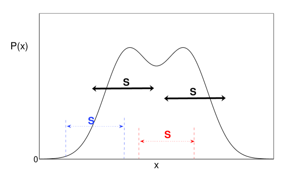
Figure 5.3: We consider an arbitrary probability distribution for a measurement $\hat{x}$ that gives a macroscopic range of outcomes.

The assumption of no generalised $S$-scopic coherence (between any two outcomes of the domain for $\hat{x}$) or, equivalently, the assumption of no generalised $S$-scopic superpositions, with respect to eigenstates of $\hat{x}$, means that the state can be written in the form

$$\rho_{S}=\sum_{i}\wp_{i}\rho_{Si},$$ (5.29)

Here each $\rho_{Si}$ is the density operator for a pure quantum state that is not such a generalised $S$-scopic superposition, so that $\rho_{Si}$ has a range of possible outcomes for $\hat{x}$ separated by less than $S$. Hence $\rho_{Si}=|\psi_{Si}\rangle\langle\psi_{Si}|$ where

$$|\psi_{Si}\rangle=\sum_{k}c_{k}|x_{k}\rangle$$ (5.30)

but the maximum separation of any two states $|x_{k}\rangle$,$|x_{k^{\prime}}\rangle$ involved in the superposition (that is with $c_{k},c_{k^{\prime}}\neq 0$ ) is less than $S$, so $|x_{k}-x_{k^{\prime}}|<S$.

Assumption (5.29) will imply a constraint on the measurable statistics, namely that there is a minimum level of uncertainty in the prediction for the complementary observable $\hat{p}$. The variances of each $\rho_{Si}$ must be bounded by

$$\Delta{{}^{2}}_{Si}x<\frac{S{{}^{2}}}{4}.$$ (5.31)

It is also true that

$$\Delta^{2}p\geq\sum_{i}\wp_{i}\Delta{{}^{2}}_{Si}p.$$ (5.32)

Now the Heisenberg uncertainty relation applies to each $\rho_{Si}$ (the inequality also applies to the MUT’s discussed in Section 5.4) so for the incompatible observables $\hat{x}$ and $\hat{p}$

$$\Delta{{}^{2}}_{Si}x\Delta{{}^{2}}_{Si}p\geq 1.$$ (5.33)

Thus a lower bound on the variance of $p$ follows.

$$\Delta^{2}p \geq \sum_{i}\wp_{i}\Delta{{}^{2}}_{Si}p$$

$$\geq \sum_{i}\wp_{i}\frac{1}{\Delta_{Si}^{2}x}>\frac{4}{S^{2}}.$$

We thus arrive at the following theorem.

Theorem 4: The assumption of no generalised $S$-scopic coherence in $\hat{x}$ will imply the following inequality for the variance of outcomes of the complementary observable $\hat{p}$:

$$\Delta p>\frac{2}{S}.$$ (5.35)

The main result of this section follows from Theorem 4 and is that the observation of a squeezing $\Delta p$ in $\hat{p}$ such that

$$\Delta p\leq 2/S$$ (5.36)

will imply the existence of an $S$-scopic superposition

$$c_{x}|x\rangle+c_{x+S}|x+S\rangle+......$$ (5.37)

namely, of a superposition of eigenstates $|x\rangle$ of $\hat{x}$, that give predictions for $\hat{x}$ with a range of at least $S$. The parameter $S$ gives a minimum extent of quantum indeterminacy with respect to the observable $\hat{x}$. Here $c_{x}$ and $c_{x+S}$ represent non-zero probability amplitudes.

In fact, using our criterion (5.36) squeezing in $p$ ($\Delta p<1$) will rule out any expansion of the system density operator in terms of superpositions of $|x\rangle$ with $S\leq 2$ (Fig. 4). Thus onset of squeezing is evidence of the onset of quantum superpositions of size $S>2$, the size $S=2$ corresponding to the vacuum noise level. This noise level may be taken as a level of reference in determining the relative size of the superposition. The experimental observation [114] of squeezing levels of $\Delta p\approx 0.4$ confirms superpositions of size at least $S=5$.

5.6.2 Bipartite systems

For composite systems comprised of two subsystems $A$ and $B$ upon which measurements $X^{A}$, $P^{A}$, $X^{B}$, $P^{B}$ can be performed, the approach of the previous section leads to the following theorem.

Theorem 5a. The assumption of no generalised $S$-scopic coherence with respect to $X^{A}$ implies

$$\Delta_{inf}p^{A}>\frac{2}{S}.$$ (5.38)

$\Delta_{inf}^{2}p^{A}$ is defined as in (5.21). The result also holds on replacing $\Delta_{inf}^{2}p^{A}$ with $\Delta_{inf,L}^{2}p^{A}$ as defined in (5.20).

Theorem 5b. The assumption of no generalised $S$-scopic coherence with respect to $\hat{x}=(X^{A}+X^{B})/\sqrt{2}$ implies

$$\Delta(\frac{p^{A}+p^{B}}{\sqrt{2}})>\frac{2}{S}.$$ (5.39)

Proof: The proof follows as for Theorem 4, but using the uncertainty relations (5.20) and (5.25) in (5.6.1) instead of (5.33). $\blacksquare$

The observation of squeezing such that (5.38) is violated, i.e

$$\Delta_{inf}p^{A}\leq 2/S$$ (5.40)

will imply the existence of an $S$-scopic superposition

$$c_{x}|x\rangle_{A}|u_{1}\rangle_{B}+c_{x+S}|x+S\rangle_{A}|u_{2}\rangle_{B}+......$$ (5.41)

namely, of a superposition of eigenstates $|x\rangle_{A}$ that give predictions for $X^{A}$ separated by at least $S$. Similarly, the observation of two-mode squeezing such that (5.39) is violated, i.e.

$$\Delta(\frac{p^{A}+p^{B}}{\sqrt{2}})\leq 2/S,$$ (5.42)

will imply existence of an $S$-scopic superposition of eigenstates of the normalised position sum $(X^{A}+X^{B})/\sqrt{2}$.

5.7 Criteria for generalised $S$-scopic coherent state superpositions

The criteria developed in the previous section may be used to rule out that a system is describable as a mixture of coherent states, or certain superpositions of them. If a system can be represented as a mixture of coherent states $|\alpha\rangle$ the density operator for the quantum state will be expressible as

$$\rho=\int P(\alpha)|\alpha\rangle\langle\alpha|d{}^{2}\alpha$$ (5.43)

which is, since $P(\alpha)$ is positive for a mixture, the Glauber-Sudarshan P-representation [48, 113]. The quadratures $\hat{x}$ and $\hat{p}$ are defined as $x=a+a^{\dagger}$ and $p=(a-a^{\dagger})/i$, so that $\Delta x=\Delta p=1$ for this minimum uncertainty state, where here $a$, $a^{\dagger}$ are the standard boson creation and annihilation operators, so that $a|\alpha\rangle=\alpha|\alpha\rangle$. Proving failure of mixtures of these coherent states would be a first requirement in a search for macroscopic superpositions, since such mixtures expand the system density operator in terms of states with equal yet minimum uncertainty in each of $x$ and $p$, that therefore do not allow significant macroscopic superpositions in either.

The coherent states form a basis for the Hilbert space of such bosonic fields, and any quantum density operator can thus be expanded as a mixture of coherent states or their superpositions. It is known [116] that systems exhibiting squeezing ($\Delta p<1$) cannot be represented by a positive Glauber-Sudarshan representation, and hence onset of squeezing implies the existence of some superposition of coherent states. A next step is to rule out mixtures of $s_{\alpha}$-scopic superpositions of coherent states . To define what we mean by this, we consider superpositions

$$|\psi_{s_{\alpha}}\rangle=\sum_{i}c_{i}|\alpha_{i}\rangle$$ (5.44)

where for any $|\alpha_{i}\rangle$, $|\alpha_{j}\rangle$ such that $c_{i},c_{j}\neq 0$, we have $|\alpha_{i}-\alpha_{j}|\leq s_{\alpha}$ for all $i$, $j$ ($s_{\alpha}$ is a positive number). We note that for a coherent state $|\alpha\rangle,$ $\langle x\rangle=2\alpha$. Thus the separation of the states with respect to $\hat{x}$ is defined as $S_{\alpha}=2s_{\alpha}$. The “separation” of the two coherent states $|-\alpha\rangle$ and $|\alpha\rangle$ (where $\alpha$ is real) in terms of $x$ corresponds to $S_{\alpha}=4\alpha=2s_{\alpha}$, as illustrated in Fig. 5.5.

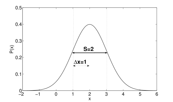
Figure 5.4: P(x) for a coherent state $|\alpha\rangle$: $\Delta x=\Delta p=1$.

We next ask whether the density operator for the system can be described in terms of the $s_{\alpha}$-scopic coherent superpositions, so that

$$\rho=\sum_{r}\wp_{r}|\psi_{s_{\alpha}}^{r}\rangle\langle\psi_{s_{\alpha}}^{r}|,$$ (5.45)

where each $|\psi_{s_{\alpha}}^{r}\rangle$ is of the form (5.44). Each $|\psi_{s_{\alpha}}^{r}\rangle$ predicts a variance in $x$ which has an upper limit given by that of the superposition $(1/\sqrt{2})\{e^{i\pi/4}|-s_{\alpha}/2\rangle+e^{-i\pi/4}|s_{\alpha}/2\rangle\}$. This state predicts a probability distribution $P(x)=\frac{1}{2}\sum_{\pm}P_{G\pm}(x)$ where

$$P_{G\pm}(x)=\frac{1}{\sqrt{2\pi}}\exp[\frac{-(x-\pm s_{\alpha})^{2}}{2}]$$ (5.46)

(Fig. 5.5), which corresponds to a variance $\Delta^{2}x=\langle x^{2}\rangle=1+s_{\alpha}^{2}=1+S_{\alpha}^{2}/4$. This means each $|\psi_{s_{\alpha}}^{r}\rangle$ is constrained to allow only $\Delta^{2}x\leq 1+s_{\alpha}^{2}$, which implies for each $|\psi_{s,r}\rangle$ a lower bound on the variance $\Delta^{2}p$ so that $\Delta^{2}p\geq 1/\Delta^{2}x\geq 1/(1+s_{\alpha}^{2})$. Thus using the result for a mixture (5.45), we get that if indeed (5.45) can describe the system, the variance in $p$ is constrained to satisfy $\Delta^{2}p\geq 1/(1+s_{\alpha}^{2})$.

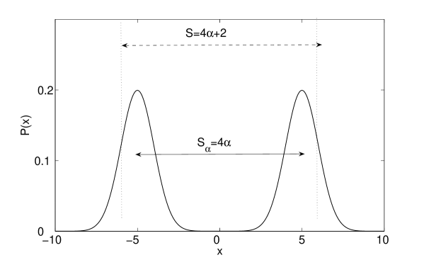
Figure 5.5: (a) P(x) for a superposition of coherent states $(1/\sqrt{2})\{e^{i\pi/4}|-\alpha\rangle+e^{-i\pi/4}|\alpha\rangle\}$ (here the scale is such that $\Delta x=1$ for the coherent state $|\alpha\rangle$).

Thus observation of squeezing $\Delta^{2}p<1$, so that the inequality

$$\Delta^{2}p<1/(1+s_{\alpha}^{2})$$ (5.47)

is violated, will allow deduction of superpositions of coherent states with separation at least $s_{\alpha}$. This separation corresponds to a separation of $S_{\alpha}=2s_{\alpha}$ in $x$ between the two corresponding Gaussian distributions (Fig. 5.5), on the scale where $\Delta^{2}x=1$ is the variance predicted by each coherent state.

We note that measured values of squeezing $\Delta p\approx 0.4$ [114] would imply $s_{\alpha}\gtrsim 2.2$. This confirms the existence of a superposition of type

$$|\psi_{S}\rangle=\sum_{i}c_{i}|\alpha_{i}\rangle=c_{-}|-\alpha_{0}\rangle+...+c_{+}|\alpha_{0}\rangle$$ (5.48)

where a separation of at least $s_{\alpha}=|\alpha_{i}-\alpha_{j}|=2.2$ occurs between two coherent states comprising the superposition, so that we may write $\alpha_{0}=1.1$. Note we have defined reference axes in phase space selected so that the $x$-axis is the line connecting the two most separated states $|\alpha_{i}\rangle$and $|\alpha_{j}\rangle$so that $|\alpha_{i}-\alpha_{j}|=2\alpha_{0}$ and the $p$-axis cuts bisects this line. The (5.48) can be compared with experimental reports [85] of generation of extreme coherent superpositions of type $(1/\sqrt{2})\{e^{i\pi/4}|-\alpha_{0}\rangle+e^{-i\pi/4}|\alpha_{0}\rangle\}$ where $|\alpha_{0}|^{2}=0.79$, implying $\alpha_{0}=0.89$. The corresponding generalised $s_{\alpha}-$scopic superposition (5.48) as confirmed by the squeezing measurement involves at least the two extreme states with $|\alpha_{0}|^{2}=1.2$, but could include other coherent states with $|\alpha_{0}|<1.1$.

5.8 Predictions of particular quantum states

We will now consider experimental tests of the inequalities derived above. An important point is that the criteria presented are sufficient to prove the existence of generalised macroscopic superpositions, but there are many macroscopic superpositions which do not satisfy the above criteria. Nevertheless there are some systems of current experimental interest which do allow for violation of the inequalities. We analyse such cases below, noting that the violation would be predicted without the experimenter needing to make assumptions about the particular state involved.

5.8.1 Coherent states

The wave function for the coherent state $|\alpha\rangle$ is

$$\left\langle x|\alpha\right\rangle=\frac{1}{(2\pi)^{\frac{1}{4}}}\exp\{\frac{-x^{2}}{4}+\alpha x-|\alpha|^{2}\}.$$ (5.49)

This gives the expansion in the continuous basis set $|x\rangle$, the eigenstates of $\hat{x}$. Thus for the coherent state

$$|\alpha\rangle=\sum_{x}c_{x}|x\rangle=\int\langle x|\alpha\rangle|x\rangle dx.$$ (5.50)

The probability distribution for $\hat{x}$ is the Gaussian (Fig. 5.4)

$$P(x)=|\langle x|\alpha\rangle|^{2}=\frac{1}{(2\pi)^{\frac{1}{2}}}\exp\{\frac{-(x-2\alpha)^{2}}{2}\},$$ (5.51)

(we take $\alpha$ to be real) centred at $2\alpha$ and with variance $\Delta^{2}x=1$

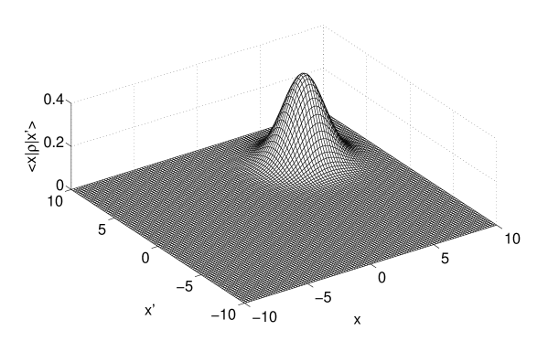
Figure 5.6: Plot of $\langle x|\rho|x^{\prime}\rangle$ for a coherent state $|\alpha\rangle$.

The coherent state possesses nonzero off-diagonal elements $\langle x|\rho|x^{\prime}\rangle$ where $|x-x^{\prime}|$ is large and thus strictly speaking can be regarded as a generalised macroscopic superposition. However, as $x$ and $x^{\prime}$ deviate from $2\alpha$, the matrix elements decay rapidly, and the off-diagonal elements decay rapidly with increasing separation.

$$\langle x|\rho|x^{\prime}\rangle=\frac{1}{(2\pi)^{\frac{1}{2}}}\exp\{\frac{-(x-2\alpha)^{2}}{4}+\frac{-(x^{\prime}-2\alpha)^{2}}{4}\}$$ (5.52)

In effect then, the off-diagonal elements become zero for significant separations $|x-x^{\prime}|\geq 1$ (Fig.5.6). We can expect that the detection of the macroscopic aspects of this superposition will be difficult. Since $\Delta p=1$, it follows that we can use the criterion (5.35) to prove coherence between outcomes of $x$ separated by at most $S=2$ (Fig. 5.4), which corresponds to the separation $S=2\Delta x$.

5.8.2 Superpositions of coherent states

The superposition of two coherent states [122, 126]

$$|\psi\rangle=(1/\sqrt{2})\{e^{i\pi/4}|-\alpha\rangle+e^{-i\pi/4}|\alpha\rangle\},$$ (5.53)

where $\alpha$ is real and large is an example of a macroscopic superposition state. The wave function in the position basis is

$$\langle x|\psi\rangle=\frac{-ie^{i\pi/4}e^{[-x^{2}/4-\alpha_{0}^{2}]}}{\sqrt{2}(2\pi)^{\frac{1}{4}}}\{e^{\alpha x}+ie^{-\alpha x}\}.$$

We consider the two complementary observables $\hat{x}$ and $\hat{p}$, and note that the probability distribution $P(x)$ for $\hat{x}$ displays two Gaussian peaks centred on $x=\pm 2\alpha$ (Fig. 5.5): $P(x)=\frac{1}{2}\sum_{\pm}P_{G\pm}(x)$ where $P_{G\pm}(x)=\exp[{-(x-\pm 2\alpha)^{2}/2}]/\sqrt{2\pi}$. Each Gaussian has variance $\Delta^{2}x=1$.

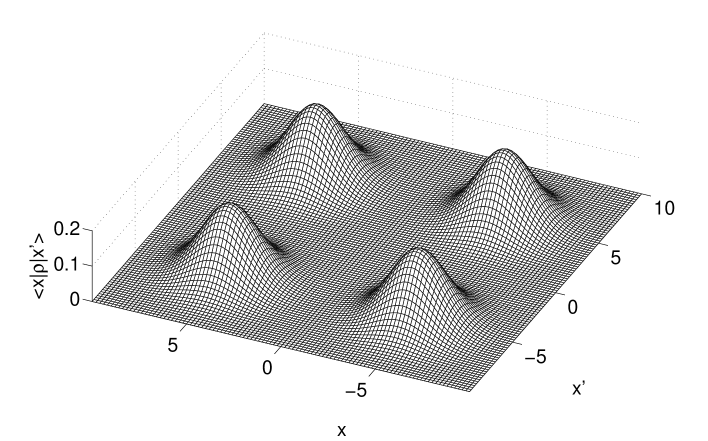
Figure 5.7: Plot of $\langle x|\rho|x^{\prime}\rangle$ for the superposition state (5.53).

The macroscopic nature of the superposition is reflected in the significant magnitude of the off-diagonal elements $\langle x|\rho|x^{\prime}\rangle$ where $x=\pm 2\alpha$ and $x^{\prime}=\mp 2\alpha$, corresponding to $|x-x^{\prime}|=4\alpha$. In fact

$$|\langle x|\rho|x^{\prime}\rangle|=\frac{e^{\frac{-(x^{2}+x^{\prime 2})}{4}-2\alpha_{0}^{2}}}{\sqrt{2\pi}}\sqrt{\cosh(2\alpha x)\cosh(2\alpha x^{\prime})},$$ (5.54)

as is plotted in Fig. 5.7 and which for these values of $x$ and $x^{\prime}$ becomes $\frac{(1-e^{-8\alpha^{2}})}{2(2\pi)^{\frac{1}{2}}}$. With significant off-diagonal elements connecting macroscopically different values of $x$, this superposition is a good example of a generalised macroscopic superposition (5.7).

Nonetheless we show that the simple linear criteria (5.35) and (5.17) derived from (B.1) are not sufficiently sensitive to detect the extent of the macroscopic coherence of this superposition state (5.53), even though the state (5.53) cannot be written in the form (5.10). We point out that it may be possible to derive further nonlinear constraints from (5.10) to arrive at more sensitive criteria.

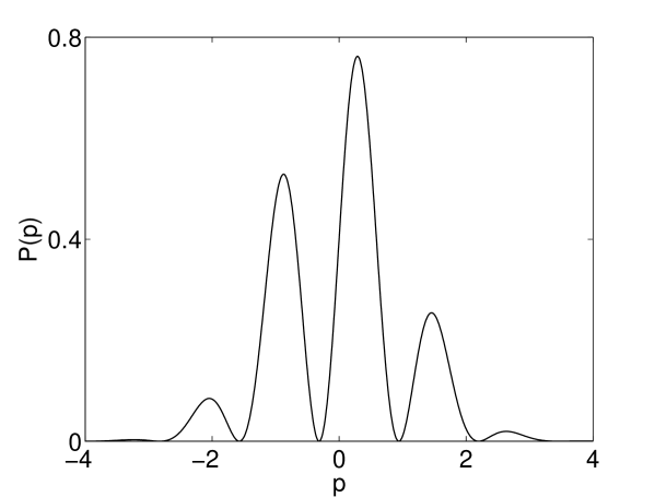
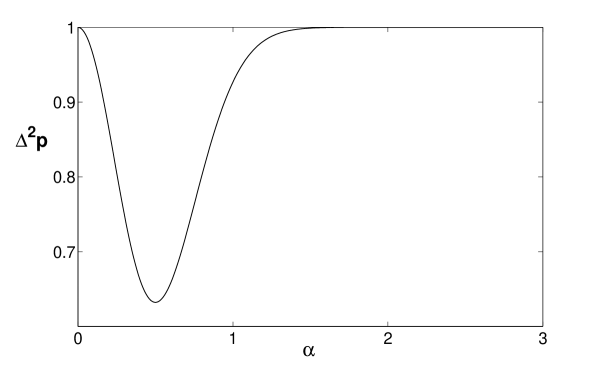
Figure 5.8: (a) P(p) for a superposition (5.53) of two coherent states where $\alpha=2.5$ and (b) the reduced variance $\Delta^{2}p<1$, versus $\alpha$.

To investigate what can be inferred from criteria (5.35), we note that $\hat{x}$ is the macroscopic observable. The complementary observable $\hat{p}$ has distribution $P(p)=\exp{[-p^{2}/2]}(1+\sin{2\alpha p)}/\sqrt{2\pi}$ which exhibits fringes and has variance $\Delta^{2}p=1-4\alpha^{2}\exp{[-4\alpha^{2}]}$ (Fig. 5.8). There is a maximum squeezing of $\Delta^{2}p\approx 0.63$ at $\alpha=0.5$. However, the squeezing diminishes as $\alpha$ increases, so the criterion becomes less effective as the separation of states of the macroscopic superposition increases. The maximum separation $S$ that could be conclusively inferred from this criterion is $S\approx 2.5$ at $\alpha=0.5$.

As discussed in Section 5.7, the detection of squeezing in $p$ is enough to confirm the system is not that of the mixture

$$\rho=1/2(|\alpha\rangle\langle\alpha|+|-\alpha\rangle\langle-\alpha|)$$ (5.55)

of the two coherent states. In fact, the squeezing rules out that the system is any mixture of coherent states. We note though that since the degree of squeezing $\Delta p$ is small, our criteria is not sensitive enough to rule out superpositions of macroscopically separated coherent states.

5.8.3 Squeezed states

Consider the single-mode momentum squeezed state[127]

$$|\psi\rangle=e^{r(a{{}^{2}}-a^{\dagger 2})}\left|0\right\rangle.$$ (5.56)

Here $\left|0\right\rangle$ is the vacuum state. For large values of $r$ these states are generalised macroscopic superpositions of the continuous set of eigenstates $|x\rangle$ of $\hat{x}=a+a^{\dagger}$, with wave function

$$\left\langle x|\psi\right\rangle=\frac{1}{(2\pi\sigma)^{\frac{1}{4}}}\exp\{\frac{-x^{2}}{4\sigma}\},$$ (5.57)

and associated Gaussian probability distribution

$$P(x)=\frac{1}{(2\pi\sigma)^{\frac{1}{2}}}\exp\{\frac{-x^{2}}{2\sigma}\}.$$ (5.58)

The variance is $\sigma=e^{2r}$. As the squeeze parameter $r$ increases, the probability distribution expands, so that eventually with large enough $r$, $x$ can be regarded as a macroscopic observable. This behaviour is shown in Fig. 5.9. The distribution for $p$ is also Gaussian but is squeezed, meaning that it has reduced variance: $\Delta^{2}p<1$. In fact, the (5.56) is a minimum uncertainty state, with $\Delta^{2}p=1/\sigma=e^{-2r}$. Where squeezing is significant, the off-diagonal elements $\langle x|\rho|x^{\prime}\rangle=\langle x|\psi\rangle\langle\psi|x^{\prime}\rangle$ (where $|x-x^{\prime}|$ is large) are significant over a large range of $x$ values (Fig. 5.9).

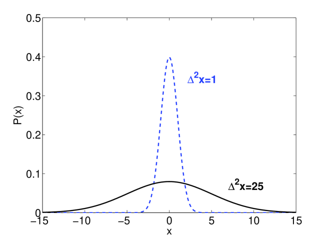
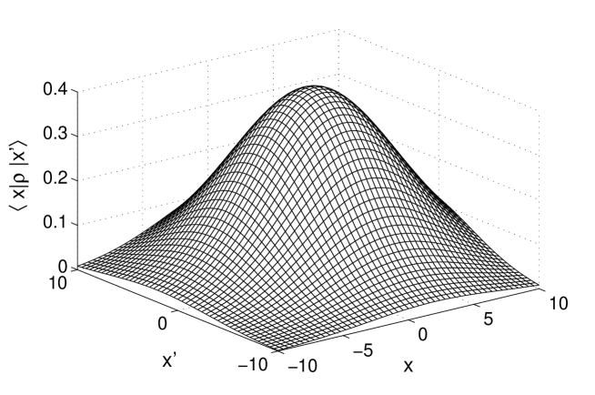
Figure 5.9: (a) Probability distribution for a measurement $X$ for a momentum-squeezed state. The variance $\Delta^{2}x$ increases with squeezing in $p$, to give a macroscopic range of outcomes, and for the minimum uncertainty state (5.56) satisfies $\Delta x\Delta p=1$. (b) The $\langle x|\rho|x^{\prime}\rangle$ for a squeezed state (5.56) with $r=13.4$ ($\Delta x=3.67)$ which predicts $\langle a^{\dagger}a\rangle=2.5^{2}$.

The criterion (5.17) for the binned outcomes is violated for the ideal squeezed state (5.56) for values of $S$ up to $0.5\sqrt{\sigma}$. The criterion can thus confirm macroscopic superpositions of states with separation of up to half the standard deviation of the probability distribution of $x$, even as $\Delta x\rightarrow\infty$. This behaviour has been reported in [28] and is shown in Fig. 5.10.

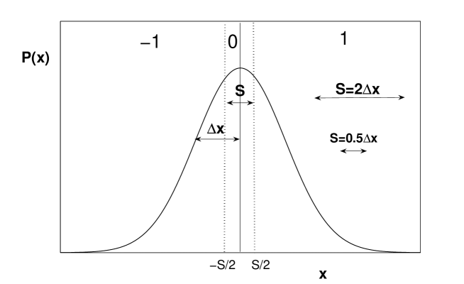
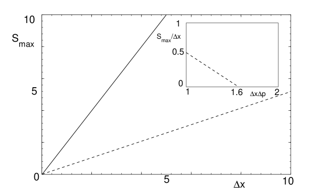
Figure 5.10: Detection of underlying superpositions of size $S$ for the squeezed minimum uncertainty state (5.56) by violation of (5.17) (dashed line of (b)) and (5.35) (full line of (b)). $S_{max}$ is the maximum $S$ for which the inequalities are violated. Inset of (b) shows behaviour of violation of (5.17) for general Gaussian-squeezed states. Inequality (5.35) depends only on $\Delta p$. The size of $S_{max}$ relative to $P(x)$ is illustrated in (a).

Squeezed systems that are generated experimentally will not be describable as the pure squeezed state (5.56). This pure state is a minimum uncertainty state with $\Delta x\Delta p=1$. Typically experimental data will generate Gaussian probability distributions for both $x$ and $p$ and with squeezing $\Delta p<1$ in $p$, but typically $\Delta x\Delta p>1$. The maximum value of $S$ that can be proved in this case of the Gaussian states reduces to $0$ as $\Delta x\Delta p$ (or $\Delta x\Delta_{inf}p$) increases to $\sim 1.6$. This is shown in Fig. 5.10. Analysis of recent experimental data for impure states that allows a violation of (5.17) has been reported by Marquardt et al [75].

The criterion (5.35), as given by Theorem 4, is better able to detect the superpositions (Fig. 5.10), particularly where the uncertainty product gives $\Delta x\Delta p>1$, though in this case the superpositions are non-locatable in phase space, so that we cannot conclude an outcome domain for the states involved in the superposition. This criterion depends only on the squeezing $\Delta p$ in the one quadrature and is not sensitive to the product $\Delta x\Delta p$. For ideal squeezed states with variance $\Delta^{2}x=\sigma$, one can prove a superposition of size $S=2\sqrt{\sigma}$, four times that obtained from (5.17) (Fig. 5.10).

Experimental reports [114] of squeezing of orders $\Delta p\approx 0.4$ confirms superpositions of size at least $S=5$, which is 2.5 times that defined by $S=2$, which corresponds to two standard deviations of the coherent state, for which $\Delta x=1$ (Fig. 5.4).

5.8.4 Two-mode squeezed states

Next we consider the two- mode squeezed state [31]

$$e^{r(ab-a^{\dagger}b^{\dagger})}|0\rangle|0\rangle.$$ (5.59)

Here $a,b$ are boson annihilation operators for modes $A$ and $B$ respectively. The wave function $\langle x|\psi\rangle$ and distribution $P(x)$ are as in (5.57) and (5.58), but the variance in $\hat{x}=X^{A}$ is now given by $\sigma=\cosh 2r$. The $\hat{x}=X^{A}$ is thus a macroscopic observable.

In the two-mode case, the squeezing is in a linear combination $P^{A}+P^{B}$ of the momenta $P^{A}$ and $P^{B}$ at $A$ and $B$, rather than in the momentum $\hat{p}=P^{A}$ for $A$ itself. The observable that is complementary to $X^{A}$ is of form $\tilde{P}=P^{A}-gP^{B}$ where $g$ is a constant, which is (5.19) of Section 5.5. We can select to evaluate one of the criteria (5.23), (5.38) or (5.39).

Choosing as our macroscopic observable $X^{A}$ and our complementary one $P^{A}-gP^{B}$, we calculate

$$\Delta_{inf}^{2}p^{A}=1/\sigma=1/cosh2r$$ (5.60)

for the choice $g=\left\langle P^{A}P^{B}\right\rangle/\left\langle(P^{B})^{2}\right\rangle=-tanhr$ which minimises $\Delta_{inf}^{2}p^{A}$ [96]. The application of results to criterion (5.23) gives the result as in Fig. 5.10, to indicate detection of superpositions of size $S$ where $S=0.5\sqrt{\sigma}$ for the ideal squeezed state (5.59), and the result shown in the inset of Fig. 5.9 if $\Delta x^{A}\Delta_{inf}p^{A}>1$.

The prediction for the criterion of Theorem 3, to detect superpositions in the position sum $X^{A}+X^{B}$ by measurement of a narrowed variance in the momenta sum $P^{A}+P^{B}$, is also given by the results of Fig. 5.10. Calculation for the ideal state (5.59) predicts $\Delta^{2}(\frac{p^{A}+p^{B}}{\sqrt{2}})=e^{-2r}$ and $\Delta^{2}(\frac{x^{A}+x^{B}}{\sqrt{2}})=e^{+2r}$ which corresponds to that of the single-mode squeezed state. The prediction for the maximum value of $S$ of Theorem 3 is therefore given by the dashed curves of Fig. 5.10, and the inset.

A better result is given by (5.38), if we are not concerned with the location of the superposition. Where we use (5.38), the degree of reduction in $\Delta_{inf}^{2}p^{A}$ determines the size of superposition $S$ that may be inferred. By Theorem 5, measurement of $\Delta_{inf}p^{A}$ allows inference of superpositions of eigenstates of $X^{A}$ separated by at least

$$S=2/\Delta_{inf}p^{A}.$$ (5.61)

Realistic states are not likely to be pure squeezed states as given by (5.59). Nonetheless the degree of squeezing indicates a size of superposition in $X^{A}$, as given by Theorem 5. Experimental values of $\Delta_{inf}^{2}p^{A}\approx 0.76$ have been reported [17], to give confirmation of superpositions of size $S\approx 2.3$, which is $1.1$ times the level of $S=2$ that corresponds to two standard deviations $\Delta x^{A}=1$ of the vacuum state (Fig. 5.4).

More frequently, it is the practice to measure squeezing in the direct sum $P^{A}+P^{B}$ of momenta. The macroscopic observable is the position sum $X^{A}+X^{B}$. The reports of measured experimental values indicate [68] $\Delta^{2}(\frac{p^{A}+p^{B}}{\sqrt{2}})\approx 0.4$, which according to Theorem 5 implies superpositions in $(X^{A}+X^{B})/\sqrt{2}$ of size $S\approx 3.2$, of order $1.6$ times the standard vacuum state level . The slightly better experimental result for the superpositions in the position sum may be understood since it has been shown by Bowen et al. [17] that, for the Gaussian squeezed states, the measurement of $\Delta_{inf}^{2}p^{A}$ is more sensitive to loss than that of $\Delta^{2}(p^{A}+p^{B})$. The $\Delta_{inf}p^{A}$ is an asymmetric measure that enables demonstration of the EPR paradox [96, 98], a strong form of quantum nonlocality [95, 121].

5.9 Concluding remarks

In this chapter we have derived criteria sufficient to detect generalised macroscopic (or $S$-scopic) superpositions ($\sum_{k_{1}}^{k_{2}}c_{k}|x_{k}\rangle$) of eigenstates of an observable $\hat{x}$. For these superpositions, the important quantity is the value $S$ of the extent of the superposition, which is the range in prediction of the observable ($S$ is the maximum of $|x_{j}-x_{i}|$ where $c_{j},c_{i}\neq 0$). This quantity gives the extent of indeterminacy in the quantum prediction for $\hat{x}$. In this sense, there is a contrast with the prototype macroscopic superposition ( of type $c_{2}|x_{2}\rangle+c_{1}|x_{1}\rangle$) that relates directly to the essay of Schrödinger [104]. Such a prototype superposition contains only the two states that have separation $S$ in their outcomes for $x$. Nonetheless, we have discussed how the generalised superposition is relevant to testing the ideas of Schrödinger, in that such macroscopic superpositions are shown to be inconsistent with the hypothesis of a quantum system being in at most one of two macroscopically separated states.

We have also defined the concept of a generalised $S$-scopic coherence and the class of Minimum Uncertainty Theories without direct reference to quantum mechanics. The former is introduced in Section 5.2 as the assumption (5.3) and is associated to the failure of a generalised assumption of macroscopic reality. This assumption is that the system is in at most one of two macroscopically distinguishable states, but that these underlying states are not specified to be quantum states. The assumption of Minimum Uncertainty Theories is that these component states do at least satisfy the quantum uncertainty relations. In the derivation of the criteria of this chapter, only two assumptions are made: that the system does satisfy this generalised macroscopic ($S$-scopic) reality and that the theory is a Minimum Uncertainty Theory. These assumptions lead to inequalities, which, when violated, generate evidence that at least one of the assumptions must be incorrect.

We point out that if, in the event of violation of the inequalities, we opt to conclude the failure of the Minimum Uncertainty Theory assumption, then this does not imply quantum mechanics to be incorrect, but rather that it is incomplete, in the sense that the component states can themselves not be quantum states. It can be said then that violation of the inequalities of this chapter implies at least one of the assumptions of generalised macroscopic ($S$-scopic) reality and the completeness of quantum mechanics is incorrect.

There is a similarity with the Einstein-Podolsky-Rosen argument [39]. In the EPR argument, the assumption of a form of realism (local realism) is shown to be inconsistent with the completeness of quantum mechanics. Therefore, as a conclusion of that argument, one is left to conclude that at least one of local realism and the completeness of QM is incorrect [98, 120, 95]. EPR opted for the first and took their argument as a demonstration that quantum mechanics was incomplete. Only after Bell [7] was it shown that this was an incorrect choice. Here, as in the EPR argument, the assumption of a form of realism (macroscopic ($S$-scopic) realism) can only be made consistent with the predictions of quantum mechanics if one allows a kind of theory in which the underlying states are not restricted by the uncertainty relations [28].

Chapter 6 Conclusion

As mentioned in the Introduction, the objective of this thesis was to contribute to the area or research termed experimental metaphysics. Our modest contribution was in formalising old concepts, proposing new ones, and finding new results in well-studied areas. We have also proposed experiments to test each of the major results. It is experimental metaphysics, after all.

In Chapter 2 we set up the appropriate terminology and the basic concepts. Most of it were simply careful definitions of standard concepts, but some definitions were new and some results and consequences may not have been fully appreciated before.

In Chapter 3 we analysed the original argument of Einstein, Podolsky and Rosen (EPR) [39], and proposed a general mathematical form for the assumptions behind that argument, namely those of local causality and completeness of quantum theory. That entailed what was termed a Local Hidden State model by Wiseman et al. [121], which was proposed as a formalisation of the concept of steering first introduced by Schrödinger [104] in a reply to the EPR paper. Violation of any consequences that can be derived from the assumption of that model therefore implies a demonstration of the EPR paradox. We have re-derived the well-known EPR-Reid criterion [96] for continuous-variables correlations, and derived new ones applicable to the spin setting considered by Bohm [14].

The spin set-up of the EPR-Bohm paradox was used by Bell [7] to derive his now famous theorem demonstrating the incompatibility of the assumption of local causality and the predictions of quantum mechanics. The inequalities which bear his name can be derived for any number of discrete outcomes, but so far there has been no derivation which can be directly applied to the continuous-variables case of the original EPR paradox. In Chapter 4 we closed the circle by deriving a class of inequalities which make no explicit mention about the number of outcomes of the experiments involved, and can therefore be used in continuous-variables measurements with no need for binning the continuous results into discrete ones. Apart from that intrinsic interest, these inequalities could prove important as a means to perform an unambiguous test of Bell inequalities which does not suffer from the logical loopholes that plague all experimental demonstrations so far, since optical homodyne detection can be performed with high detection efficiency. The technique, which is based on a simple variance inequality, was also used to re-derive a large class of well-known Bell-type inequalities and at the same time find their quantum bound, making explicit from a formal point of view that the non-commutativity of the local operators is at the heart of the quantum violations.

Finally, in Chapter 5 we addressed the issue of macroscopic superpositions originally sparked by the infamous "cat paradox" of Schrödinger [104], presented in the same seminal paper where he coined the terms entanglement and steering. We considered macroscopic, mesoscopic and ‘S-scopic’ quantum superpositions of eigenstates of an observable, and developed some signatures for their existence. We defined the extent, or size S of a (pure-state) superposition, with respect to an observable X, as being the maximum difference in the outcomes of X predicted by that superposition. Such superpositions were referred to as generalised S-scopic superpositions to distinguish them from the extreme superpositions that superpose only the two states that have a difference S in their prediction for the observable. We also considered generalised S-scopic superpositions of coherent states. We explored the constraints that are placed on the statistics if we suppose a system to be described by mixtures of superpositions that are restricted in size. In this way we arrived at experimental criteria that are sufficient to deduce the existence of a generalised S-scopic superposition. The signatures developed are useful where one is able to demonstrate a degree of squeezing.

Appendix A Proof of Theorem A of Chapter 5

We will now prove the statement that coherence between $x_{1}$ and $x_{2}$ is equivalent to a nonzero off-diagonal element $\langle x_{1}|\rho|x_{2}\rangle$ in the density matrix. As discussed in section 5.2, within quantum mechanics the statement that there exists coherence between $x_{1}$ and $x_{2}$ is equivalent to the statement that there is no decomposition of the density matrix of form (5.2) where $\rho_{1}$ and $\rho_{2}$ are density matrices such that $\langle x_{1}|\rho_{2}|x_{1}\rangle=\langle x_{2}|\rho_{1}|x_{2}\rangle=0$. Therefore Theorem A can be reformulated as saying that $\langle x_{1}|\rho|x_{2}\rangle=0$ iff such a decomposition does exist.

It’s easy to prove the first direction of the equivalence: if $\exists$$\{\wp_{1},\,\wp_{2},\,\rho_{1},\,\rho_{2}\}$ such that $\rho=\wp_{1}\rho_{1}+\wp_{2}\rho_{2}$ and $\langle x_{1}|\rho_{2}|x_{1}\rangle=\langle x_{2}|\rho_{1}|x_{2}\rangle=0$, then $\langle x_{1}|\rho|x_{2}\rangle=0$. To show this, first note that for any density matrix $\bar{\rho}$ and $\forall\,\{x,x^{\prime}\},$ if $\langle x|\bar{\rho}|x\rangle=0$ then $\langle x|\bar{\rho}|x^{\prime}\rangle=0,$ where $\langle x|x^{\prime}\rangle=\delta_{x,x^{\prime}}$. Since by assumption $\langle x_{1}|\rho_{2}|x_{1}\rangle=\langle x_{2}|\rho_{1}|x_{2}\rangle=0$, then $\langle x_{1}|\rho|x_{2}\rangle=\sum_{i}\wp_{i}\langle x_{1}|\rho_{i}|x_{2}\rangle=0$.

The converse can also be proved. We use the facts that any $\rho$ can always be written as the reduced density matrix of an enlarged pure state, where the system of interest (call it $A$) is entangled with an ancilla $B$, i.e,

$$\rho=Tr_{B}\{|\Psi\rangle_{AB}\langle\Psi|_{AB}\}$$ (A.1)

and that any bipartite pure state can always be written in the Schmidt decomposition [37]

$$|\Psi\rangle_{AB}=\sum_{i}\sqrt{\eta_{i}}|\psi_{i}\rangle|\phi_{i}^{B}\rangle.$$ (A.2)

where $\{|\psi_{i}\rangle\}$ and $\{|\phi_{i}^{B}\rangle\}$ are orthonormal and $\eta_{i}\in[0,1].$ The superscript $B$ denotes the states of the ancilla and the absence of a superscript denotes the states of the system of interest, $A$. We decompose each pure state $|\psi_{i}\rangle$ that appears in the Schmidt decomposition in the basis of eigenstates of $\hat{x}$ as $|\psi_{i}\rangle=\sum_{k}c_{i,k}|x_{k}\rangle$. By assumption $\langle x_{1}|\rho|x_{2}\rangle=0$ and therefore $\sum_{i}\eta_{i}\langle x_{1}|\psi_{i}\rangle\langle\psi_{i}|x_{2}\rangle=\sum_{i}\eta_{i}c_{i,1}c_{i,2}^{*}=0$. We can expand $|\Psi_{AB}\rangle$ as

$$|\Psi_{AB}\rangle=|x_{1}\rangle|\tilde{1_{B}}\rangle+|x_{2}\rangle|\tilde{2_{B}}\rangle+\sum_{k>2,\,i}\sqrt{\eta_{i}}c_{i,k}|x_{k}\rangle|\phi_{i}^{B}\rangle,$$ (A.3)

where we define the (unnormalized) $|\tilde{1_{B}}\rangle\equiv\sum_{i}\sqrt{\eta_{i}}c_{i,1}|\phi_{i}^{B}\rangle$ and $|\tilde{2_{B}}\rangle\equiv\sum_{i}\sqrt{\eta_{i}}c_{i,2}|\phi_{i}^{B}\rangle$. The inner product of these two vectors is $\langle\tilde{1_{B}}|\tilde{2_{B}}\rangle=\sum_{i}\eta_{i}c_{i,1}c_{i,2}^{*}.$ But as shown above $\sum_{i}\eta_{i}c_{i,1}c_{i,2}^{*}=0$, so $|\tilde{1_{B}}\rangle$ and $|\tilde{2_{B}}\rangle$ are orthogonal. We can therefore define an orthonormal basis with the (normalized) $|1_{B}\rangle=|\tilde{1_{B}}\rangle/\sqrt{\sum_{i}\eta_{i}|c_{i,1}|^{2}}$ and $|2_{B}\rangle=|\tilde{2_{B}}\rangle/\sqrt{\sum_{i}\eta_{i}|c_{i,2}|^{2}},$ plus additional $|j_{B}\rangle$with $3\leq j\leq D$, where $D$ is the dimension of subsystem $B$’s Hilbert space. Taking the trace of $\rho_{AB}=|\Psi_{AB}\rangle\langle\Psi_{AB}|$ therefore yields

$$\rho = Tr_{B}\{\rho_{AB}\}$$ (A.4)

$$= \left\langle 1_{B}\right|\rho_{AB}\left|1_{B}\right\rangle+\left\langle 2_{B}\right|\rho_{AB}\left|2_{B}\right\rangle$$

$$+\sum_{j>2}\left\langle j_{B}\right|\rho_{AB}\left|j_{B}\right\rangle.$$

Now referring to expansion (A.3), we see that $\langle 1_{B}|\rho_{AB}|1_{B}\rangle=\sum_{i}\eta_{i}|c_{i,1}|^{2}|x_{1}\rangle\langle x_{1}|$ and $\langle 2_{B}|\rho_{AB}|2_{B}\rangle=\sum_{i}\eta_{i}|c_{i,2}|^{2}|x_{2}\rangle\langle x_{2}|.$ We then define $\rho_{1}\equiv|x_{1}\rangle\langle x_{1}|,$ $\wp_{1}\equiv\sum_{i}\eta_{i}|c_{i,1}|^{2},$ $\wp_{2}=1-\wp_{1}$ and $\rho_{2}\equiv\frac{1}{\wp_{2}}\{\sum_{i}\eta_{i}|c_{i,2}|^{2}|x_{2}\rangle\langle x_{2}|+\sum_{j>2}\langle j_{B}|\rho_{AB}|j_{B}\rangle\}.$ Obviously $\langle x_{2}|\rho_{1}|x_{2}\rangle=0,$ and by substituting (A.3) into $\rho_{2}$ we see that $\langle x_{1}|\rho_{2}|x_{1}\rangle=0.$ Therefore $\rho$ can be decomposed as $\rho=\wp_{1}\rho_{1}+\wp_{2}\rho_{2}$ with $\langle x_{1}|\rho_{2}|x_{1}\rangle=\langle x_{2}|\rho_{1}|x_{2}\rangle=0$ as desired.

Appendix B Proof of Theorem 2 of Chapter 5

We wish to prove that if $\rho$ can be written as

$$\rho=\wp_{L}\rho_{L}+\wp_{R}\rho_{R},$$ (B.1)

then

$$\Delta_{inf}^{2}p^{A}\geq\wp_{L}\Delta_{inf,L}^{2}p^{A}+\wp_{R}\Delta_{inf,R}^{2}p^{A}$$ (B.2)

where

$$\Delta_{inf,J}^{2}p^{A}=\sum_{p^{B}}P_{J}(p^{B})\Delta_{J}^{2}(p^{A}|p^{B}).$$

The subscript $J$ refers to the $\rho_{J}$ from which the probabilities are calculated.

We have

$$\Delta_{inf}^{2}p^{A} = \sum_{p^{B}}P(p^{B})\Delta^{2}(p^{A}|p^{B})$$

$$= \sum_{p^{B}}\sum_{p^{A}}P(p^{A},p^{B})(p^{A}-\langle p^{A}|p^{B}\rangle)^{2}$$

$$= \sum_{p^{B}}\sum_{p^{A}}\sum_{I=R,L}\wp_{I}P_{I}(p^{A},p^{B})(p^{A}-\langle p^{A}|p^{B}\rangle)^{2}$$

$$\geq \sum_{p^{B}}\sum_{p^{A}}\sum_{I=R,L}\wp_{I}P_{I}(p^{A},p^{B})(p^{A}-\langle p^{A}|p^{B}\rangle_{I})^{2}$$

The inequality follows because $\langle p^{A}|p^{B}\rangle$ is the mean of $P(p^{A}|p^{B})$ for the $\rho$ of (B.1), and the choice $a=\sum_{p}P(p)p=\langle p\rangle$ will minimise $\sum_{p}P(p)(p-a)^{2}$. From this the desired result follows.

References

- AGM [06] A. Acin, N. Gisin, and L. Masanes, From Bell’s theorem to secure quantum key distribution, Physical Review Letters 97 (2006), no. 12, 120405.
- AGMS [04] A. Acin, N. Gisin, L. Masanes, and V. Scarani, Bell’s inequalities detect efficient entanglement, International Journal of Quantum Information 2 (2004), no. 1, 23–31.
- AMM+ [03] A. Auffeves, P. Maioli, T. Meunier, S. Gleyzes, G. Nogues, M. Brune, J. M. Raimond, and S. Haroche, Entanglement of a mesoscopic field with an atom induced by photon graininess in a cavity, Physical Review Letters 91 (2003), no. 23, 230405.
- AMRS [02] G. Auberson, G. Mahoux, S. M. Roy, and V. Singh, Bell inequalities in phase space and their violation in quantum mechanics, Physics Letters A 300 (2002), no. 4-5, 327–333.
- Ard [92] M. Ardehali, Bell inequalities with a magnitude of violation that grows exponentially with the number of particles, Physical Review A 46 (1992), no. 9, 5375–5378.
- Arn [05] Frank Arntzenius, Reichenbach’s common cause principle, The Stanford Encyclopedia of Philosophy (Spring 2005 Edition) (Edward N. Zalta, ed.), 2005.
- Bel [64] J. S. Bell, On the Einstein-Podolsky-Rosen paradox, Physics 1 (1964), 195.
- Bel [87] , Speakable and unspeakable in quantum mechanics, Cambridge University Press, 1987.
- BHD+ [96] M. Brune, E. Hagley, J. Dreyer, X. Maitre, A. Maali, C. Wunderlich, J. M. Raimond, and S. Haroche, Observing the progressive decoherence of the ”meter” in a quantum measurement, Physical Review Letters 77 (1996), no. 24, 4887–4890.
- BHK [05] J. Barrett, L. Hardy, and A. Kent, No signaling and quantum key distribution, Physical Review Letters 95 (2005), no. 1, 010503.
- BHU+ [02] B. Brezger, L. Hackermuller, S. Uttenthaler, J. Petschinka, M. Arndt, and A. Zeilinger, Matter-wave interferometer for large molecules, Physical Review Letters 88 (2002), no. 10, 100404.
- BK [93] A. V. Belinskii and D. N. Klyshko, Iinterference of light and Bell’s theorem, Physics-Uspekhi 36 (1993), 653.
- BM [06] G. Brassard and A. A. Méthot, Can quantum-mechanical description of physical reality be considered incomplete?, International Journal of Quantum Information 4 (2006), no. 1, 45–54.
- Boh [51] D. Bohm, Quantum theory, ch. 22, Prentice Hall, Englewood Cliffs, N.J., 1951.
- Bor [71] Max Born, The Born-Einstein letters, Walker, 1971.
- BSBL [02] W. P. Bowen, R. Schnabel, H. A. Bachor, and P. K. Lam, Polarization squeezing of continuous variable stokes parameters, Physical Review Letters 88 (2002), no. 25, 093601.
- BSLR [03] W. P. Bowen, R. Schnabel, P. K. Lam, and T. C. Ralph, Experimental investigation of criteria for continuous variable entanglement, Physical Review Letters 90 (2003), no. 4, 043601.
- BW [99] K. Banaszek and K. Wodkiewicz, Testing quantum nonlocality in phase space, Physical Review Letters 82 (1999), no. 10, 2009–2013.
- BZPZ [04] C. Brukner, M. Zukowski, J. W. Pan, and A. Zeilinger, Bell’s inequalities and quantum communication complexity, Physical Review Letters 92 (2004), no. 12, 127901.
- Cab [02] A. Cabello, Bell’s inequality for n spin-s particles, Physical Review A 65 (2002), no. 6, 062105.
- CDH+ [06] J. F. Corney, P. D. Drummond, J. Heersink, V. Josse, G. Leuchs, and U. L. Andersen, Many-body quantum dynamics of polarization squeezing in optical fibers, Physical Review Letters 97 (2006), no. 2, 023606.
- CG [04] D. Collins and N. Gisin, A relevant two qubit Bell inequality inequivalent to the CHSH inequality, Journal of Physics A-Mathematical and General 37 (2004), no. 5, 1775–1787.
- CGL+ [02] D. Collins, N. Gisin, N. Linden, S. Massar, and S. Popescu, Bell inequalities for arbitrarily high-dimensional systems, Physical Review Letters 88 (2002), no. 4, 040404.
- CHSH [69] J. F. Clauser, M. A. Horne, A. Shimony, and R. A. Holt, Proposed experiment to test local hidden-variable theories, Physical Review Letters 23 (1969), no. 15, 880.
- CL [85] A. O. Caldeira and A. J. Leggett, Influence of damping on quantum interference: an exactly soluble model, Physical Review A 31 (1985), no. 2, 1059–1066.
- CM [89] James T. Cushing and Ernan McMullin (eds.), Philosophical consequences of quantum theory, Studies in science and the humanities from the Reilly Center for Science, Technology and Values, vol. 2, University of Notre Dame press, 1989.
- CPHZ [02] Z. B. Chen, J. W. Pan, G. Hou, and Y. D. Zhang, Maximal violation of Bell’s inequalities for continuous variable systems, Physical Review Letters 88 (2002), no. 4, 040406.
- CR [06] E. G. Cavalcanti and M. D. Reid, Signatures for generalized macroscopic superpositions, Physical Review Letters 97 (2006), no. 17, 170405.
- CR [07] , Uncertainty relations for the realization of macroscopic quantum superpositions and EPR paradoxes, Journal of Modern Optics 54 (2007), 2373.
- CS [78] J. F. Clauser and A. Shimony, Bell’s theorem - experimental tests and implications, Reports on Progress in Physics 41 (1978), no. 12, 1881–1927.
- CS [85] C. M. Caves and B. L. Schumaker, New formalism for 2-photon quantum optics .1. quadrature phases and squeezed states, Physical Review A 31 (1985), no. 5, 3068–3092.
- DGCZ [00] L. M. Duan, G. Giedke, J. I. Cirac, and P. Zoller, Inseparability criterion for continuous variable systems, Physical Review Letters 84 (2000), no. 12, 2722–2725.
- DM [98] F. De Martini, Amplification of quantum entanglement, Physical Review Letters 81 (1998), no. 14, 2842–2845.
- DMSS [05] F. De Martini, F. Sciarrino, and V. Secondi, Realization of an optimally distinguishable multiphoton quantum superposition, Physical Review Letters 95 (2005), no. 24, 240401.
- Dow [00] Phil Dowe, Physical causation, Cambridge University Press, 2000.
- Dru [83] P. D. Drummond, Violations of Bell’s inequality in cooperative states, Physical Review Letters 50 (1983), 1407.
- EK [95] A. Ekert and P. L. Knight, Entangled quantum-systems and the Schmidt decomposition, American Journal of Physics 63 (1995), no. 5, 415.
- Eke [91] A. K. Ekert, Quantum cryptography based on Bell’s theorem, Physical Review Letters 67 (1991), no. 6, 661–663.
- EPR [35] A. Einstein, B. Podolsky, and N. Rosen, Can quantum-mechanical description of physical reality be considered complete?, Physical Review 47 (1935), 777.
- Eve [57] H. Everett, Relative state formulation of quantum mechanics, Reviews of Modern Physics 29 (1957), 454–462.
- Fin [82] A. Fine, Hidden-variables, joint probability, and the Bell inequalities, Physical Review Letters 48 (1982), no. 5, 291–295.
- FPC+ [00] J. R. Friedman, V. Patel, W. Chen, S. K. Tolpygo, and J. E. Lukens, Quantum superposition of distinct macroscopic states, Nature 406 (2000), no. 6791, 43–46.
- Fur [36] W. H. Furry, Note on the quantum-mechanical theory of measurement, Physical Review 49 (1936), no. 5, 0393–0399.
- GBP [98] N. Gisin and H. Bechmann-Pasquinucci, Bell inequality, Bell states and maximally entangled states for n qubits, Physics Letters A 246 (1998), no. 1-2, 1–6.
- GDR [98] A. Gilchrist, P. Deuar, and M. D. Reid, Contradiction of quantum mechanics with local hidden variables for quadrature phase amplitude measurements, Physical Review Letters 80 (1998), no. 15, 3169–3172.
- Gis [91] N. Gisin, Bell inequality holds for all non-product states, Physics Letters A 154 (1991), no. 5-6, 201–202.
- Gis [07] N. Gisin, Bell inequalities: many questions, a few answers, e-print:quant-ph/0702021 (2007).
- Gla [63] R. J. Glauber, Coherent and incoherent states of radiation field, Physical Review 131 (1963), no. 6, 2766.
- GM [87] A. Garg and N. D. Mermin, Detector inefficiencies in the Einstein-Podolsky-Rosen experiment, Physical Review D 35 (1987), 3831.
- GPFC+ [04] R. Garcia-Patron, J. Fiurasek, N. J. Cerf, J. Wenger, R. Tualle-Brouri, and P. Grangier, Proposal for a loophole-free Bell test using homodyne detection, Physical Review Letters 93 (2004), no. 13, 130409.
- GPR [90] G. C. Ghirardi, P. Pearle, and A. Rimini, Markov-processes in hilbert-space and continuous spontaneous localization of systems of identical particles, Physical Review A 42 (1990), no. 1, 78–89.
- GRW [86] G. C. Ghirardi, A. Rimini, and T. Weber, Unified dynamics for microscopic and macroscopic systems, Physical Review D 34 (1986), no. 2, 470–491.
- HBBB [04] J. C. Howell, R. S. Bennink, S. J. Bentley, and R. W. Boyd, Realization of the Einstein-Podolsky-Rosen paradox using momentum- and position-entangled photons from spontaneous parametric down conversion, Physical Review Letters 92 (2004), no. 21, 210403.
- Hei [30] W. Heinsenberg, The physical principles of quantum mechanics, The University of Chicago Press, 1930.
- HHH [95] R. Horodecki, P. Horodecki, and M. Horodecki, Violating Bell inequality by mixed spin-1/2 states - necessary and sufficient condition, Phys. Lett. A 200 (1995), no. 5, 340–344.
- HHH [96] R. Horodecki, M. Horodecki, and P. Horodecki, Teleportation, Bell’s inequalities and inseparability, Phys. Lett. A 222 (1996), no. 1-2, 21–25.
- HS [07] N. Harrigan and R. W. Spekkens, Einstein, incompleteness, and the epistemic view of quantum states, arXiv:0706.2661 (2007).
- HT [03] H. F. Hofmann and S. Takeuchi, Violation of local uncertainty relations as a signature of entanglement, Physical Review A 68 (2003), no. 3, 032103.
- Jar [84] J. P. Jarrett, On the physical significance of the locality conditions in the Bell-arguments, Nous 18 (1984), no. 4, 569–589.
- JCKL [06] S. S. Jang, Y. W. Cheong, J. Kim, and H. W. Lee, Physical Review A 74 (2006), 062112.
- JDB+ [04] V. Josse, A. Dantan, A. Bramati, M. Pinard, and E. Giacobino, Continuous variable entanglement using cold atoms, Physical Review Letters 92 (2004), no. 12, 123601.
- JDV+ [03] V. Josse, A. Dantan, L. Vernac, A. Bramati, M. Pinard, and E. Giacobino, Polarization squeezing with cold atoms, Physical Review Letters 91 (2003), no. 10, 103601.
- JIKC [07] J. Dubois J. I. Korsbakken, K. B. Whaley and J. I. Cirac, Measurement-based measure of the size of macroscopic quantum superpositions, Physical Review A 75 (2007), 042106.
- JKP [01] B. Julsgaard, A. Kozhekin, and E. S. Polzik, Experimental long-lived entanglement of two macroscopic objects, Nature 413 (2001), no. 6854, 400–403.
- JSC+ [04] B. Julsgaard, J. Sherson, J. I. Cirac, J. Fiurasek, and E. S. Polzik, Experimental demonstration of quantum memory for light, Nature 432 (2004), no. 7016, 482–486.
- Kor [07] N. Korolkova, Polarization squeezing and entanglement, Quantum Information with continuous variables of atoms and light (N. J. Cerf, G. Leuchs, and E. S. Polzik, eds.), Imperial College Press, 2007, pp. 181–196.
- LBS+ [04] D. Leibfried, M. D. Barrett, T. Schaetz, J. Britton, J. Chiaverini, W. M. Itano, J. D. Jost, C. Langer, and D. J. Wineland, Toward Heisenberg-limited spectroscopy with multiparticle entangled states, Science 304 (2004), no. 5676, 1476–1478.
- LCK+ [05] J. Laurat, T. Coudreau, G. Keller, N. Treps, and C. Fabre, Physical Review A 71 (2005), 022313.
- Leg [84] A. J. Leggett, Schrödinger’s cat and her laboratory cousins, Contemporary Physics 25 (1984), 583.
- Leg [02] A. J. Leggett, Testing the limits of quantum mechanics: motivation, state of play, prospects, Journal of Physics-Condensed Matter 14 (2002), no. 15, R415–R451.
- LG [85] A. J. Leggett and A. Garg, Quantum mechanics versus macroscopic realism: Is the flux there when nobody looks?, Physical Review Letters 54 (1985), 857.
- LLHB [01] A. Lamas-Linares, J. C. Howell, and D. Bouwmeester, Stimulated emission of polarization-entangled photons, Nature 412 (2001), no. 6850, 887–890.
- LPZB [04] W. Laskowski, T. Paterek, M. Zukowski, and C. Brukner, Tight multipartite Bell’s inequalities involving many measurement settings, Physical Review Letters 93 (2004), no. 20, 200401.
- LV [95] U. Leonhardt and J. A. Vaccaro, Bell correlations in phase-space: application to quantum optics, J. Mod. Opt. 42 (1995), no. 5, 939–943.
- MAL+ [07] C. Marquardt, U. L. Andersen, G. Leuchs, Y. Takeno, M. Yukawa, H. Yonezawa, and Furusawa A., Experimental demonstration of macroscopic quantum coherence in gaussian states, Physical Review A 76 (2007), 030101(R).
- Mau [94] Tim Maudlin, Quantum non-locality and relativity, Blackwell, 1994.
- Mer [80] N. D. Mermin, Quantum-mechanics vs local realism near the classical limit: a Bell inequality for spin-s, Physical Review D 22 (1980), no. 2, 356–361.
- Mer [90] N. D. Mermin, Extreme quantum entanglement in a superposition of macroscopically distinct states, Physical Review Letters 65 (1990), 1838.
- MMKW [96] C. Monroe, D. M. Meekhof, B. E. King, and D. J. Wineland, A ”Schrodinger cat” superposition state of an atom, Science 272 (1996), no. 5265, 1131–1136.
- MSPB [03] W. Marshall, C. Simon, R. Penrose, and D. Bouwmeester, Towards quantum superpositions of a mirror, Physical Review Letters 91 (2003), no. 13, 130401.
- NLP [06] K. Nagata, W. Laskowski, and T. Paterek, Bell inequality with an arbitrary number of settings and its applications, Physical Review A 74 (2006), no. 6, 062109.
- [82] T. Norsen, Against ’realism’, Foundations of Physics 37 (2007), no. 3, 311–340.
- [83] T. Norsen, J. S. Bell’s concept of Local Causality, arxiv:0707.0401v1 (2007).
- OPKP [92] Z. Y. Ou, S. F. Pereira, H. J. Kimble, and K. C. Peng, Realization of the Einstein-Podolsky-Rosen paradox for continuous-variables, Physical Review Letters 68 (1992), no. 25, 3663–3666.
- OTBLG [06] A. Ourjoumtsev, R. Tualle-Brouri, J. Laurat, and P. Grangier, Generating optical Schrodinger kittens for quantum information processing, Science 312 (2006), no. 5770, 83–86.
- Per [78] A. Peres, Unperformed experiments have no results, American Journal of Physics 46 (1978), no. 77, 745–747.
- Per [92] A. Peres, Emergence of local realism in fuzzy observations of correlated quantum-systems, Foundations of Physics 22 (1992), no. 6, 819–828.
- Per [99] , All the Bell inequalities, Foundations of Physics 29 (1999), no. 4, 589–614.
- Pit [89] I. Pitowsky, Quantum probability - quantum logic, Lecture Notes in Physics, vol. 321, Springer-Verlag, 1989.
- Pop [94] S. Popescu, Bell inequalities versus teleportation: what is nonlocality, Physical Review Letters 72 (1994), no. 6, 797–799.
- PR [92] S. Popescu and D. Rohrlich, Generic quantum nonlocality, Physics Letters A 166 (1992), no. 5-6, 293–297.
- Pri [96] Huw Price, Time’s arrow and archimedes’ point, Oxford University Press, New York, 1996.
- RBH [01] J. M. Raimond, M. Brune, and S. Haroche, Colloquium: Manipulating quantum entanglement with atoms and photons in a cavity, Reviews of Modern Physics 73 (2001), no. 3, 565–582.
- RC [05] M. D. Reid and E. G. Cavalcanti, Macroscopic quantum Schrodinger and Einstein-Podolsky-Rosen paradoxes, Journal of Modern Optics 52 (2005), no. 16, 2245–2252.
- [95] M. D. Reid, P. D. Drummond, W. P. Bowen, P. K. Lam, H. A. Bachor, U. L. Anderson, and G. Leuchs, to be published.
- Rei [89] M. D. Reid, Demonstration of the Einstein-Podolsky-Rosen paradox using nondegenerate parametric amplification, Physical Review A 40 (1989), no. 2, 913–923.
- Rei [01] , Bell inequalities with Schrodinger cats, Zeitschrift fur Naturforschung A 56 (2001), no. 1-2, 220–223.
- Rei [03] , Einstein-Podolsky-Rosen correlations, entanglement and quantum cryptography, Quantum Squeezing (P. D. Drummond and Ficek Z., eds.), Springer-Verlag, 2003.
- RMDM [02] M. D. Reid, W. J. Munro, and F. De Martini, Violation of multiparticle Bell inequalities for low- and high-flux parametric amplification using both vacuum and entangled input states, Physical Review A 66 (2002), no. 3, 033801.
- Rov [96] C. Rovelli, Relational quantum mechanics, International Journal of Theoretical Physics 35 (1996), no. 8, 1637–1678.
- RRH+ [04] C. F. Roos, M. Riebe, H. Haffner, W. Hansel, J. Benhelm, G. P. T. Lancaster, C. Becher, F. Schmidt-Kaler, and R. Blatt, Control and measurement of three-qubit entangled states, Science 304 (2004), no. 5676, 1478–1480.
- SBK [06] W. Son, C. Brukner, and M. S. Kim, Test of nonlocality for a continuous-variable state based on an arbitrary number of measurement outcomes, Physical Review Letters 97 (2006), no. 11, 110401.
- SBRF [93] D. T. Smithey, M. Beck, M. G. Raymer, and A. Faridani, Measurement of the wigner distribution and the density-matrix of a light mode using optical homodyne tomography: application to squeezed states and the vacuum, Physical Review Letters 70 (1993), no. 9, 1244–1247.
- Sch [35] E. Schrödinger, Die gegenwärtige situation in der quantenmechanick, Naturwissenschaften 23 (1935), 807.
- SG [01] V. Scarani and N. Gisin, Quantum communication between N partners and Bell’s inequalities, Physical Review Letters 8711 (2001), no. 11, 117901.
- Shi [89] Abner Shimony, Search for a worldview which can accommodate our knowledge of microphysics, Philosophical consequences of quantum theory (James T. Cushing and Ernan McMullin, eds.), University of Notre Dame Press, 1989.
- Sim [00] R. Simon, Peres-Horodecki separability criterion for continuous variable systems, Physical Review Letters 84 (2000), 2726.
- SLK [06] W. Son, J. Lee, and M. S. Kim, Generic Bell inequalities for multipartite arbitrary dimensional systems, Physical Review Letters 96 (2006), no. 6, 060406.
- SLW+ [01] C. Silberhorn, P. K. Lam, O. Weiss, F. Konig, N. Korolkova, and G. Leuchs, Generation of continuous variable Einstein-Podolsky-Rosen entanglement via the Kerr nonlinearity in an optical fiber, Physical Review Letters 86 (2001), no. 19, 4267–4270.
- SSP [02] C. Schori, J. L. Sorensen, and E. S. Polzik, Physical Review A 66 (2002), 033802.
- Sta [77] H. P. Stapp, Are superluminal connections necessary?, Nuovo Cimento 40B (1977), 191–205.
- SU [07] M. Seevinck and J. Uffink, Local commutativity versus Bell inequality violation for entangled states and versus non-violation for separable states, e-print: quant-ph/0703134 (2007).
- Sud [63] E. C. G. Sudarshan, Equivalence of semiclassical and quantum mechanical descriptions of statistical light beams, Physical Review Letters 10 (1963), no. 7, 277.
- SYK+ [06] S. Suzuki, H. Yonezawa, F. Kannari, M. Sasaki, and A. Furusawa, 7 db quadrature squeezing at 860 nm with periodically poled ktiopo4, Applied Physics Letters 89 (2006), no. 6, 061116.
- Tot [04] G. Toth, Entanglement detection in optical lattices of bosonic atoms with collective measurements, Physical Review A 69 (2004), no. 5.
- Wal [83] D. F. Walls, Squeezed states of light, Nature 306 (1983), no. 5939, 141–146.
- Wer [89] R. F. Werner, Quantum states with Einstein-Podolsky-Rosen correlations admitting a hidden-variable model, Physical Review A 40 (1989), no. 8, 4277–4281.
- WHG+ [03] J. Wenger, M. Hafezi, F. Grosshans, R. Tualle-Brouri, and P. Grangier, Maximal violation of Bell inequalities using continuous-variable measurements, Physical Review A 67 (2003), no. 1, 012105.
- Wic [95] David Wick, The infamous boundary, Birkhauser, 1995.
- Wis [06] H. M. Wiseman, From Einstein’s theorem to Bell’s theorem: a history of quantum non-locality, Contemporary Physics 47 (2006), no. 2, 79–88.
- WJD [07] H. M. Wiseman, S. J. Jones, and A. C. Doherty, Steering, entanglement, nonlocality, and the einstein-podolsky-rosen paradox, Physical Review Letters 98 (2007), no. 14, 140402.
- WM [85] D. F. Walls and G. J. Milburn, Effect of dissipation on quantum coherence, Physical Review A 31 (1985), no. 4, 2403–2408.
- WS [50] C. S. Wu and I. Shaknov, The angular correlation of scattered annihilation radiation, Physical Review 77 (1950), no. 1, 136–136.
- WW [01] R. F. Werner and M. M. Wolf, All-multipartite Bell-correlation inequalities for two dichotomic observables per site, Physical Review A 6403 (2001), no. 3, 032112.
- YHS [99] B. Yurke, M. Hillery, and D. Stoler, Position-momentum local-realism violation of the Hardy type, Physical Review A 60 (1999), no. 5, 3444–3447.
- YS [86] B. Yurke and D. Stoler, Generating quantum mechanical superpositions of macroscopically distinguishable states via amplitude dispersion, Physical Review Letters 57 (1986), 13–16.
- Yue [76] H. P. Yuen, 2-photon coherent states of radiation-field, Physical Review A 13 (1976), no. 6, 2226–2243.
- Zuk [93] M. Zukowski, Bell theorem involving all settings of measuring apparatus, Physics Letters A 177 (1993), no. 4-5, 290–296.
- Zuk [06] M. Zukowski, All tight multipartite Bell correlation inequalities for three dichotomic observables per observer, e-print:quant-ph/0611086 (2006).
- Zur [91] W. H. Zurek, Decoherence and the transition from quantum to classical, Physics Today 44 (1991), no. 10, 36–44.
- Zur [03] , Decoherence, einselection, and the quantum origins of the classical, Reviews of Modern Physics 75 (2003), no. 3, 715–775.
- ZWL+ [00] Y. Zhang, H. Wang, X. Y. Li, J. T. Jing, C. D. Xie, and K. C. Peng, Experimental generation of bright two-mode quadrature squeezed light from a narrow-band nondegenerate optical parametric amplifier, Physical Review A 6202 (2000), no. 2, 023813.