Competition between Surface Energy and Elastic Anisotropies in the Growth of Coherent Solid State Dendrites

Abstract

A new phase field model of microstructural evolution is presented that includes the effects of elastic strain energy. The model’s thin interface behavior is investigated by mapping it onto a recent model developed by Echebarria et al [2]. Exploiting this thin interface analysis the growth of solid state dendrites are simulated with diffuse interfaces and the phase field and mechanical equilibrium equations are solved in real space on an adaptive mesh. A morphological competition between surface energy anisotropy and elastic anisotropy is examined. Two dimensional simulations are reported that show that solid state dendritic structures undergo a transition from a surface dominated [10] growth direction to an elastically driven [11] growth direction by changes in the elastic anisotropy, the surface anisotropy and the supersaturation. Using the curvature and strain corrections to the equilibrium interfacial composition and linear stability theory for isotropic precipitates as calculated by Mullins and Sekerka, the dominant growth morphology is predicted.

I Introduction

Recent years have seen the increased use of phase field modeling of free-boundary problems related to microstructure growth. This method has the advantage in that it avoids explicit front tracking by making phase boundaries spatially diffuse through the use of one or more order parameters, $\phi$, which vary continuously across interfaces. This method of simulation has been very successful in modeling dendritic solidification [4, 26]. In particular, Phase Field theory has confirmed the predictions of the microscopic solvability theory of dendrite growth [8, 9, 10]. That is, the anisotropy in the surface energy ($\gamma$), although small, controls the growth rate and morphology of the resultant precipitate [20].

More recently the phase field approach has been used to study dendrite growth directions in cases where multiple sources of anisotropy can compete to control the resultant morphological structure. Haxhimali et al. [30] showed that the dendrite growth direction in Al-Zn alloys can change continuously from (100) to (110) with the addition of solute. The authors explained their observations as an interplay between the four fold and six fold anisotropy parameters [12], was conjectured to vary as a function of solute. Analogously, Provatas et al. [27] modeled the change from (100) directed dendirites to a seaweed structure as the surface energy anisotropy competed with the direction of the temperature gradient.

The phase field method has also been used to model the effects of elastic and plastic effects on microstructural evolution [3, 13, 17, 31, 32, 36, 11]. In these studies the elastic strain energy was added to the phase field energy functional and the elastic modulus tensor ($C_{ijkl}$) was assumed to be a function of the phase field $\phi$. Many of these studies have focused on the interaction of elastic fields on growth and coarsening rates of solid state particles [33, 16]. These studies have shown that elastic effects play an important role in controlling growth rates and morphology, consistent with previous analytical predictions of Laraia et al. [14] and Voorhees et al [35]. Energy minimization techniques also showed that the elastic free energy drives the interface to become unstable for mismatched elastic coefficients under both applied and self strain [18, 19]. Other studies have also incorporated the effect of mobile dislocations in phase field modeling [23]. They have examined such effects as the role of dislocations on the coarsening rate during spinoidal decomposition [24].

Another phenomenon of both scientific and practical interest, and that has has not received enough theoretical study, concerns the morphology and growth rate of solid state dendrites when two sources of anisotropy can compete. Anisotorpy can result from the surface energy ($\gamma$) or the more interesting result of anisotropy emerging in the elastic modulus tensor ($C_{ijkl}$). Experimentally it has been found that dendritic structures can appear in the solid state [15, 34] provided specific elastic and kinetic relationships between the parent and precipitate phases are met. As discussed by Husain et al. [34], solid state dendrites are made possible if the precipitating phase and the parent phase have similar atomic lattice structures, there is a high rate of atomic transfer between the two phases and the transformation rate is controlled by diffusion in the presence of an anisotropy. More exotic structures can also be found through competing mechanisms leading to interface instabilities as shown by Yoo [37].

This paper studies solid state dendritic growth in the presence of competitive interactions between surface energy and elastic anisotropy. It quantifies a transition between dominant growth morphologies controlled by each of these two anisotropic effects. Section II presents the phase field model used in this study. Section III examines the effect of isotropic strains on the equilibrium composition. Section IV provides an approximation to the anisotropic strain field at the interface of the precipitate. Section V illustrates the effect of the surface energy anisotropy, elastic energy anisotropy and supersaturation on the growth morphology of dendritic growth. Finally, the transition between a surface energy controlled morphology and an elastic energy controlled morphology is quantified in Section VI.

II Phase Field Model

This section derives a phase field free energy for solid state transformations, which assumed a dilute alloy free energy for the bulk chemical thermodynamics. To this is added an additional contribution to account for elastic free energy. Corresponding phase field equations are then derived from this free energy. It is shown that the phase parameters can be related according according to the thin interface asymptotics of Ref. [2] to a good approximation. The thin interface limit allows for significant efficiency of simulations of the phase field equations, particularly when combined with novel adaptive mesh refinement algorithms [28, 1].

The bulk chemical free energy is given by

$$G(\phi,C,\epsilon_{ij})=f(T_{m})-S(\phi)(T-T_{m})$$

$$+\frac{RT}{\nu}\left(c\ln c-c\right)+E(\phi)c+f_{el}(\phi)$$ (1)

$C$, $\phi$ and $\epsilon_{ij}$ are the solute concentration, order parameter and total strain fields, respectively. The parameter $R$ is the gas constant, $\nu$ is the molar volume, $T$ is the temperature and $T_{m}$ i the melting temperature of component $A$ of a dilute binary alloy. The elastic free energy is defined by Hooke’s law, given by

$$f_{el}(\phi)=C_{ijkl}(\phi)(\epsilon_{ij}-\epsilon_{ij}^{*}(\phi))(\epsilon_{kl}-\epsilon_{kl}^{*}(\phi))$$ (2)

where $\epsilon_{ij}^{*}(\phi)$ is the phase dependent eigenstrain, given by $\left(\epsilon^{*}_{ij}(\phi)=\frac{1+g(\phi)}{2}\epsilon^{*A}_{ij}+\frac{1-g(\phi)}{2}\epsilon^{*B}_{ij}\right)$. Here $\epsilon^{*A,B}_{ij}=\epsilon^{*}\delta_{ij}$ is the hydrostatic lattice eigenstrain with $\epsilon^{*}=\frac{a_{A}-a_{B}}{a_{A}}$ and $a_{i}$ is the lattice parameters in each phase. The phase dependent elastic tensor is interpolated across the interface by $C_{ijkl}=\frac{1+g(\phi)}{2}C_{ijkl}^{A}+\frac{1-g(\phi)}{2}C_{ijkl}^{B}$. A convenient choice for the interpolation function $g(\phi)$ which maintains the bulk phases at $\phi=\pm 1$ is given as

$$g(\phi)=\frac{15}{8}\left(\phi-\frac{2}{3}\phi^{3}+\frac{1}{5}\phi^{5}\right)$$ (3)

The elastic energy can be re-cast as a function of $g(\phi)$, leaving the elastic free energy in the form of

$$f_{el}={\it Z_{3}}\left(g(\phi)\right)^{3}+{\it Z_{2}}\left(g\left(\phi\right)\right)^{2}+{\it Z_{1}}g(\phi)+{\it Z_{0}}$$ (4)

Each pre-factor in the polynomial of $g(\phi)$ (i.e., $Z_{3}$, $Z_{2}$, $Z_{1}$ and $Z_{0}$) is a function dependent on the elastic modulus tensor. Explicit expressions for these prefactors are given in the appendix (Appendix A) for the cubic elastic modulus tensor in two-dimensions.

It is straightforward to show using the common tangent technique that the equilibrium composition, denoted $C_{b}^{eq}$, is modified by elasticity according to,

$${\it C_{b}}=C_{b}^{eq}-G_{ele}={\frac{\left(T-{\it T_{m}}\right)L\nu}{{{\it T_{m}}}TR\left(1-k\right)}}-\frac{2\nu}{TR}{\frac{\left({\it Z3}+{\it Z1}\right)}{\left(1-k\right)}}$$ (5)

where ${\it C_{b}^{eq}}={\frac{\left(T-{\it Tm}\right)L\nu}{{{\it T_{m}}}TR\left(1-k\right)}}$ is the equilibrium coexistence line corresponding to the parent phase in the absence of elasticity, $G_{ele}=\frac{2\nu}{TR}{\frac{\left({\it Z3}+{\it Z1}\right)}{\left(1-k\right)}}$ is the correction to the phase diagram due to a local change in the strain and $k=\frac{C_{A}^{eq}}{C_{B}^{eq}}$ is the partition coefficient.

II.1 A Phase Field Model For Elastically Influenced Phase Transformations

By applying the usual dissipative dynamics for the order parameter, mass conservation for concentration and strain relaxation for the strains, the following kinetic equations for the order parameter $\phi$, undercooling $U\equiv\frac{e^{u}-1}{1-k}$ (where $k$ is the partition coefficient and $u$ is defined in below) and the strain fields $\epsilon_{ij}$ are derived:
Phase Mobility:

$$\tau A(\hat{n})^{2}\frac{\partial\phi}{\partial t}=\hat{\nabla}\cdot[W^{2}A(\hat{n})^{2}\hat{\nabla}\phi]$$

$$+\hat{\nabla}\cdot\Big{(}|\hat{\nabla}\phi|^{2}W^{2}A(\hat{n})\frac{\partial A(\hat{n})}{\partial(\hat{\nabla}\phi)}\Big{)}$$

$$-(\phi^{3}-\phi)-\lambda(1+B)U(1-\phi^{2})^{2}$$ (6)

Chemical Diffusion:

$$\Psi\frac{\partial U}{\partial t}=\vec{\nabla}\cdot(D\tilde{q}(\phi)C_{b}\vec{\nabla}U)$$

$$+(1+(1-k)U)C_{b}\left(1+\frac{\alpha Z_{2}}{C_{b}(1-k)}\right)\frac{\partial\phi}{\partial t}$$

$$-(1+(1-k)U)\left(\frac{k+1}{1-k}-\phi\right)\frac{\partial C_{b}}{\partial t}$$ (7)

Strain relaxation:

$$\frac{\partial\sigma_{ij}}{\partial x_{j}}\equiv\frac{\partial}{\partial x_{j}}\frac{\delta G(\phi,C,\epsilon_{ij})}{\delta\epsilon_{ij}^{el}}=0$$ (8)

The explicit form of $B$ in equation 6 is

$$B=\left(\frac{\alpha Z_{1}}{(1-k)C_{b}^{eq}}-1\right)\frac{\alpha Z_{2}}{2C_{b}(1-k)}g(\phi)$$

$$-\frac{\alpha Z_{1}}{2C_{b}^{eq}(1-k)}$$ (9)

where $C_{b}$ is the equilibrium composition corrected for the strain by equation 5, i.e., $C_{b}=C_{b}^{eq}-\frac{1}{2}\frac{\alpha Z_{1}}{(1-k)}$ with $C_{b}^{eq}$ being the equilibrium composition in the absence of elasticity $\alpha=\frac{4\nu}{RT}$ ($Z_{3}$ has been neglected here, as discussed below). The quantities $W,\tau$ and $\lambda$ are the usual phase field parameters setting the dimensions of space and time [20, 2]. The function $A(\hat{n})\equiv 1+\epsilon_{4}cos(4\theta)$ controls the four-fold surface energy anisotropy, where $\theta$ is the angle of orientation between the interface normal $\hat{n}$ and a reference axis.

The dimensionless undercooling $\left(U\equiv\frac{e^{u}-1}{1-k}\right)$ in equation 7 is modified from its form in Ref. [2] to incorporate an elastic correction to the equilibrium composition. This results in

$$e^{u}=\frac{2C}{C_{b}}\left(k+1-(1-k)g(\phi)-\frac{\alpha Z_{2}}{2C_{b}}(1-g(\phi)^{2})\right)^{-1}$$ (10)

where $Z_{2}$ is the prefactor to $g(\phi)^{2}$ in the elastic free energy. The function $\Psi$ modulates the diffusion through the interface correcting for the diffuse nature of $\phi$ and is given by

$$\Psi=C_{b}(k+1-(1-k)\phi-\frac{Z_{2}\alpha}{2C_{b}}(1-\phi^{2}))$$ (11)

Two-sided diffusion is controlled by the function $\tilde{q}(\phi)=q(\phi)\frac{\Psi}{C_{b}}$ where $q(\phi)$ modulates the diffusion in the two phases, to simulate equal diffusion coefficients $q(\phi)=1$. The dimensional diffusion coefficient is denoted $D$.The value of elastic coefficients used herein is a actually reported as $\alpha C_{ijkl}$.

The phase field equations above are derived in the limit where $Z_{3}\rightarrow 0$, the condition for a small difference in the elastic coefficients in either phase. This condition also holds for all materials in which $\frac{Z_{3}}{Z_{1}}<<1$ holds. Generally speaking $Z_{1}>Z_{3}$ even in the most extreme disparities of the elastic coefficients, so this assumption is not unreasonable.

Following the procedure for the derivation of the phase field model presented in [2], the constants $W_{o}$, $\tau_{o}$ and $\lambda$ are inter-related by the asymptotic analysis of Ref. [20]. This analysis maps the phase field model above, without elasticity, onto the sharp interface limit governed by the Gibbs-Thomson condition $C_{int}=C_{eq}-\Delta Cd_{o}(\vec{n})\kappa-\Delta C\beta(\vec{n})V$, where $d_{o}$ is the capillary length, $\beta_{k}(\vec{n})$ is interface kinetic coefficient and $\Delta C$ is the concentration jump across the to phase interface. Echebarria et al. showed that for the case of vanishing kinetic coefficient (appropriate for the study of solid state denderites) the following relations must be obeyed: $\frac{d_{o}}{W}=0.8839\lambda$ and $D\equiv\bar{D}\tau/W^{2}=0.6267\lambda$ where $\bar{D}$ is the diffusion coefficient in dimensional units ($m^{2}/s$). These relationships arise by an expansion of the phase ($\phi$) and composition ($C$) inside the interface, which is matched to solutions outside the interface such as to emulate the sharp interface boundary conditions.

It expected that for the phase field model presented in this work the thin interface relationships between $W_{o}$, $\tau_{o}$ and $\lambda$ will be, to lowest order, the same as those for the model of Echebarria et al. based on two observations. The first is drawn from the work of Yeon et al. [7], who showed that, to first order, the inclusion of elasticity is decoupled from the curvature and kinetic effects in the Gibbs-Thomson condition, which reads $C_{int}=C_{eq}-\Delta Cd_{o}(\vec{n})\kappa-\Delta C\beta_{k}(\vec{n})V-G_{ele}$. In their asymptotic matching procedure the derivation of $d_{o}$ and $\beta_{k}(\vec{n})$ remained unaffected by the presence of the $G_{ele}$ contribution.

The second observations validating the use of the thin interface analysis of Ref. [2] for the phase field model presented here is that for our simulations it was foind that $\frac{\partial C_{b}}{\partial t}<<1$ in Equation 7 and $B\ll 1$ in equation 6. The first quantity was found numerically to be at least an order of magnitude smaller than the other terms in its equation. It was likewise also found that $B<<1$ (which includes $Z_{2}\ll 1$). Both $B$ and $\frac{\partial C_{b}}{\partial t}$ are zero in the limit of zero strain, but are also small for small lattice eigenstrains. For larger strains these terms are still valid as long as the interfacial velocity ($V$) is small. In effect a small velocity eliminates any excess kinetic effects that arise at the interface. In this work only small eigenstrains ($\epsilon^{*}\approx 0.005$) and small growth rates ($V<1\mu m/s$) are considered.

It should be noted that the small variable $B$ accounts for the effect of a variable strain field on the development of the precipitate. It plays an analogous role to the temperature correction of $\lambda$ that is used when simulating solidification of alloys with non-linear coexistence phase boundaries [5].

III Growth of an Isotropic Second Phase Precipitate with Coherent Interfaces in an Isotropic Parent Phase

This section examines the interface compositions of an isolated second phase precipitated into a parent phase, which is grown under isotropic conditions in both the parent and precipitate phases. The surface energy is made isotropic by setting the surface energy anisotropy coefficient $\epsilon_{4}=0$. The elasticity equations are formulated in terms of cubic tensor coefficients, ie $C_{11}$,$C_{12}$ and $C_{44}$ as described in appendix A. For isotropic linear elastic coefficients the cubic elastic terms are related by,

$$C_{44}=\frac{1}{2}(C_{11}-C_{12})$$ (12)

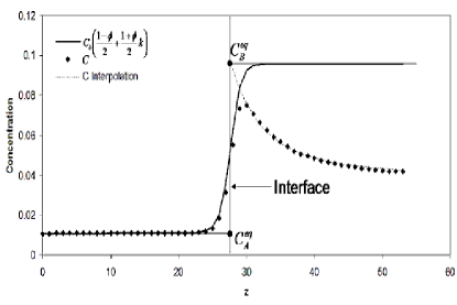
Figure 1: A circular isotropic coherent precipitate is grown in an alloy with initial composition of $C_{o}=0.04$ with a hydrostatic lattice eigenstain of $\epsilon^{*}=0.005$. A cross section of the composition is shown with the corresponding equilibrium composition corrected for strain, $C_{b}\left(\frac{1-\phi}{2}+\frac{1+\phi}{2}k\right)$. The compositions are interpolated to the center of the interface and are found to be in good agreement with the sharp interface boundary condition.

where for this simulation $C_{11}=1011$ and $C_{12}=729$ ($C_{ij}$ is dimensionalized by $\alpha$ ) and the coherent hydrostatic eigenstrain is set to $\epsilon^{*}=0.005$. The convergence constant of the phase field equations is $\lambda=3$. The equilibrium composition is $C_{b}^{eq}=0.1$ with an initial alloy composition of $C_{o}=0.04$ and the solute partition coefficient is set to a value of $k=0.1$. The diffusion coefficients are set equal in both phases thus removing the phase dependency in the diffusion coefficient (ie. $q(\phi)=1$) in equation 7.

The total domain size simulated is $6400W$ on a side with periodic boundary conditions. The phase field and diffusion equations are solved using an explicit time stepping algorithm on an adaptive mesh with a grid spacing of $dx=0.391$ at the lowest level of refinement and a time step of $dt=0.01$. The displacement field is solved by direct Gauss-Seidel iteration, which is found to require ($O(N)$) operations per time step on an adaptive mesh [22].

The precipitate particle is grown and a cross section of the composition field solved by Equation 7 is shown in Figure 1. This figure indicates the corresponding value of the equilibrium interfacial composition as calculated by equation 5. $C_{b}$ is plotted as a function of the phase by interpolating it through the interface to its corresponding precipitate side value by $C_{b}\left(\frac{1-\phi}{2}+\frac{1+\phi}{2}k\right)$. The composition field is interpolated to the interface described by the point where $\phi=0$ both from inside the precipitate bulk and from outside the precipitate in the parent phase. The points are denoted $C_{A}^{eq}$ and $C_{B}^{eq}$ and are found to have excellent agreement with the interpolations to the center of the interface.

IV Approximation of the Strain Field Around a Precipitate with Cubic Elastic Coefficients

In this section the elastic field is analyzed around a circular precipitate where the cubic elastic coefficients are equal in both the precipitate and matrix phases. The anisotropy is entered into the cubic elastic coefficients by introducing a deviation from the isotropic relation in equation 12 as defined here by,

$$C_{44}=\frac{1}{2}(C_{11}-C_{12})+\beta$$ (13)

where $\beta$ is the deviation from the isotropic elastic coefficients. $C_{11}$ and $C_{12}$ remain unchanged. While the analytical solution to the isotropic strain field has been derived for elliptical inclusions under a hydrostatic eigenstrain [6], a solution to an anisotropic precipitate under the same conditions is mathematically cumbersome do deal with [29] and is instead solved here numerically.

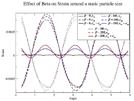
Figure 2: (Colour Online) The strain fields $\epsilon_{xx}$, $\epsilon_{yy}$ and their sum are plotted for two particle radii with $\beta=200$ in units of the model. The effect of the deviation from isotropy ($\beta=0,100,200$) on the trace of the strain tensor ($\epsilon_{xx}+\epsilon_{yy}$) is illustrated by the solid lines.

A circular precipitate in a parent phase with identical elastic coefficients in both phases is considered. The dimensionless elastic coefficients are set to values of $C_{11}=1011$ and $C_{12}=729$ ($C_{ij}$ is dimensionalized by $\alpha$, ie. $\alpha C_{ij}$), the hydrostatic eigenstrain is set to $\epsilon^{*}=0.005$ and the concentration field is made constant (The elasticity here is not influenced by compositional effects and therefore any concentration field will produce similar results). The deviation from elastic isotropy is studied by two controls, the particle radius and the strength of the deviation from isotropic elasticity ($\beta$).

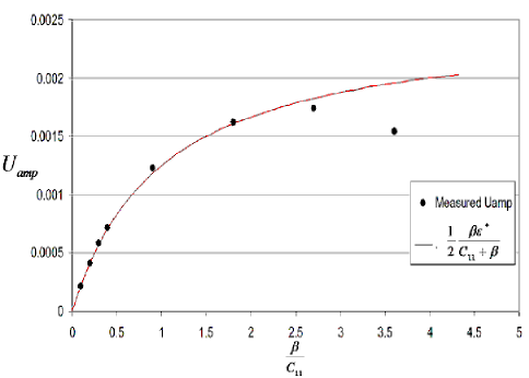
Figure 3: (Colour Online) Measured values of $U_{AMP}$ plotted vs $\frac{\beta}{C_{11}}$ and the fitted prediction of $\frac{1}{2}\frac{\beta\epsilon^{*}}{C_{11}+\beta}$.

The behaviour of the strain trace due to changes in the strength of the elastic anisotropy ($\beta$) is studied by holding the precipitate radius constant while increasing the value of $\beta$. The amplitude of the trace of the strain tensor ($\epsilon_{xx}+\epsilon_{yy})$ is found to have a strong sensitivity to variations in $\beta$. This is illustrated in Figure 2 for $\beta=0,100,200$, where the individual strain components and their sum at the precipitate/matrix interface are plotted as a function of the angle $\theta$, with zero representing the (10) direction. Notice the four fold symmetry of the trace of the strain. Although the strain energy depends strongly on the value of $\beta$, the precipitate radius is found to have little effect on the amplitude of any perturbation to the strain trace.

The $\theta$ dependence of the strain trace can be approximated to lowest order by a single Fourier mode defined by,

$$\epsilon_{xx}+\epsilon_{yy}=U_{AMP}cos(4\theta)$$ (14)

To measure the functional form for the amplitude of the strain trace ($U_{AMP}$), the anisotropic strength ($\beta$) is varied and the amplitude of the strain trace ($U_{AMP}$) is measured for the corresponding waveform at the interface of the precipitate. These measured values are fitted to a functional form, given by the equation,

$$U_{AMP}=\frac{1}{2}\frac{\beta\epsilon^{*}}{C_{11}+\beta}$$ (15)

The functional form of equation 15 shows good agreement for all values of $\beta$ in the regime where $\frac{\beta}{C_{11}}<2$ as shown in figure 3. This range of anisotropies is well within the limits of the relative anisotropic strengths that are studied here.

V Conditions Influencing the Morphology of Precipitates

This section characterizes three distinct controlling influences on the selection of a dominant morphology of precipitated dendrites. These are the anisotropies of the elastic tensor and surface energy and the supersaturation. The effect of each of these parameters are systematically tested by increasing the strength of each parameter while holding the other parameters constant.

In the following phase field simulations, $\lambda=3$ and, as required by the sharp interface analysis [2], the dimensionless diffusion coefficient is set to $D=0.6237\lambda$. The temperature is set such that the equilibrium composition is $C_{b}^{eq}=0.1$ and the partition coefficient used is $k=0.1$. The elastic coefficients were converted to units of the model by the elastic modulating factor $\alpha=6.005\cdot 10^{-9}\frac{m^{3}}{J}$ and in these units the elastic coefficients are set to a value of $C_{11}=1011$ and $C_{12}=729$, where $C_{ij}=\alpha C_{ij}$.

Precipitate structures are grown in a system with periodic boundaries, where the system size is set to $6400Wx6400W$ ($W$ being the interface width, determined along with $\tau$ from the asymptotic analysis used). The precipitates grew to sizes of at most $2000W$ and the solution to the displacement field drops off as $1/R$. This justifies the claim that purely isolated precipitates are studied while using the periodic boundaries. The diffusion coefficients and elastic coefficients have no phase dependence. The grid spacing is set to $dx=0.391W$ and the explicit time step is set to $dt=0.01\tau$.

V.1 Elastic Anisotropy ($\beta$)

The elastic anisotropy emerges from the elastic tensor ($C_{11}$, $C_{12}$ and $C_{44}=\frac{1}{2}(C_{11}-C_{12})+\beta$). The anisotropy of the tensor is varied by holding $C_{11}$, $C_{12}$ constant and varying $C_{44}$ through changes in $\beta$. Figure 4 (a-c) shows the effect of increasing the strength of the elastic anisotropy by increasing $C_{44}$ while holding surface energy anisotropy and supersaturation (controlled via the average composition $C_{o}$) constant. From top to bottom the values of $\beta$ used are $\beta=25,100,400$ respectively. As can be seen in this figure, a small elastic anisotropy causes the surface energy to dominate and the dendrite grows in the $[10]$ direction ( Figure 4 (a) ). When the elastic anisotropy is increased to sufficient strength ( Figure 4 (c) ) the dendrite grows in the $[11]$ direction. When the anisotropies effectively destructively interact the resultant structure leads to an almost isotropic growth morphology ( Figure 4 (b) ).

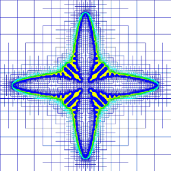
(a) $C_{o}=0.04$,$\beta=25$ and $\epsilon_{4}=0.01$

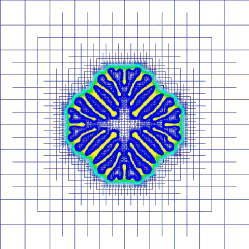
(b) $C_{o}=0.04$,$\beta=100$ and $\epsilon_{4}=0.01$

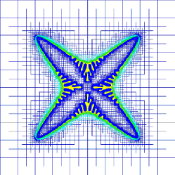
(c) $C_{o}=0.04$,$\beta=400$ and $\epsilon_{4}=0.01$

Figure 4: (Colour Online) Morphologies of growth precipitates vs. variation in the elastic anisotropy in the modulus tensor through an alteration in $\beta$. The composition field is plotted on the adaptive mesh, blue being low concentration and yellow is a higher concentration. The total system size is $6400W$, plotted is an area of $2000W$ on one side. .

V.2 Surface Energy Anisotropy ($\epsilon_{4}$)

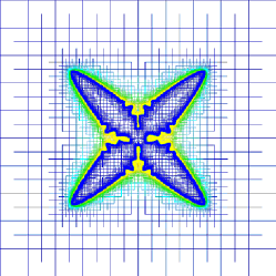
(a) $C_{o}=0.05$,$\beta=400$ and $\epsilon_{4}=0.01$

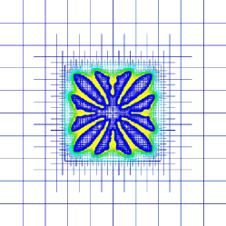
(b) $C_{o}=0.05$,$\beta=400$ and $\epsilon_{4}=0.03$

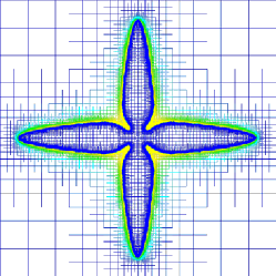
(c) $C_{o}=0.05$,$\beta=400$ and $\epsilon_{4}=0.05$

Figure 5: (Colour Online) Morphologies of growth precipitates for a variation in the surface energy anisotropy by modification of $\epsilon_{4}$. The composition field is plotted on the adaptive mesh, blue being low concentration and yellow is a higher concentration. The total system size is $6400W$, plotted is an area of $2000W$ on one side.

The surface energy anisotropy is entered into the model using the simple form for 4-fold surface energy $\gamma=\gamma_{o}(1-\epsilon_{4}cos(4\theta))$. The effect of surface energy anisotropy is examined by varying $\epsilon_{4}$ and holding both $C_{o}$ (or equivalently the super saturation $\Omega=0.555$) and the elastic anisotropy ($\beta=400$) constant. Figure 5 (a-c) shows the effect of increasing the strength of the surface anisotropy under these conditions. From top to bottom in Figure 5 the values of the $\epsilon_{4}$ used are $\epsilon_{4}=0.01,0.03,0.05$ respectively. Analogously with the effect shown in section V.1, increasing the strength of $\epsilon_{4}$ causes the morphology to transform from a preferential growth along the [11] direction ( Figure 5 (a) ) to that of the [10] direction ( Figure 5 (c) )with a transition region where the precipitate structure is isotropic ( Figure 5 (b) ).

V.3 Supersaturation($\Omega$)

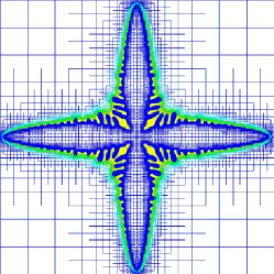
(a) $C_{o}=0.04$,$\beta=200$ and $\epsilon_{4}=0.03$

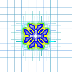
(b) $C_{o}=0.06$,$\beta=200$ and $\epsilon_{4}=0.03$

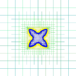
c) $C_{o}=0.08$,$\beta=200$ and $\epsilon_{4}=0.03$

Figure 6: (Colour Online) Morphologies of growth precipitates for a variation in the supersaturation with both anisotropic strengths, $\epsilon_{4}$ and $\beta$, held constant. The composition field is plotted on the adaptive mesh, blue being low concentration and yellow is a higher concentration. The total system size is $6400W$, plotted is an area of $2000W$ on one side.

The supersaturation is varied by changing the initial (i.e. average) alloy composition $C_{o}$. Figure 6 (a-c) shows the effect of decreasing the supersaturation while holding the strength of the surface anisotropy and elastic anisotropy constant. From top to bottom the values of the initial alloy composition used are $C_{o}=0.04,0.06,0.08$ respectively. For large super saturations (Figure 6 (a)) the growth direction is dominated along directions preferred by the surface energy, i.e. the [10] directions. As the supersaturation is decreased a transition from the [10] growth direction to the [11] direction is observed ( Figure 6 (b) and (c) ).

VI Characterization of the Morphological Transition

In this section we discuss a technique by which the dominant precipitate growth direction can be predicted. First, the point at which this transition occurs is defined and measured by examining the envelope of the precipitate tips in $R-\theta$ space. For a given value of the precipitate radius, analysis of the amplitude of the envelope makes it possible to determine the critical surface energy anisotropy ($\epsilon_{4}^{C}$), for a specified elastic anisotropy ($\beta$), where a morphological transition from $[10]$ to $[11]$ growth directions occurs. The elastic strain energy is, however, proportional to the precipitate area (in 2D) and the surface energy contribution varies as the particle perimeter. As such the critical $\epsilon_{4}^{C}$ is also a function of the precipitate size. The particle size dependency of $\epsilon_{4}^{C}$ vs. $\beta$ is then found by balancing the Gibbs-Thomson corrections corresponding to surface energy vs. elastic anisotropy. This critical radius scale is found to be proportional to the Mullins-Sekerka instability radius ($R^{C}$). Finally, a condition relating $\epsilon_{4}^{C}$ as a function of $\beta$ and $R^{C}$ at the transition is proposed.

VI.1 Defining the Transition Point

The transition point that characterizes the controlling mechanism of growth morphology is defined as the point at which all competing anisotropies exactly cancel. Under this condition an isolated precipitate will grow (ideally) as a circle (a sphere in three dimensions) until the interface becomes unstable by the Mullins-Sekerka instability. While in this case the interface will become unstable, the envelope around the particle will continue to grow as a spheroid. It is this envelope that allows the point of transition between anisotropically controlled directions to be characterized.

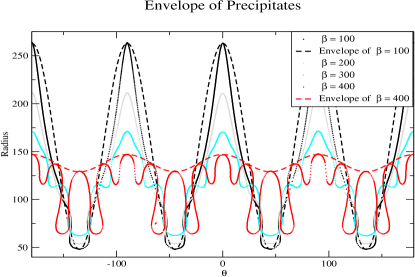
Figure 7: (Colour Online) $R$ - $\theta$ space of 4 precipitates with different $\beta$ values, $\epsilon_{4}=0.03$ and Supersaturation $=0.666$. The dashed lines illustrate the corresponding envelope of the precipitate. As the control values approach a critical point, the envelope amplitude goes to 0.

The concept of the precipitate envelope is illustrated in Figure 7 where the interface for 4 precipitates with values of $\beta=100,200,300,400$, $\epsilon_{4}=0.03$ and $\Omega=0.666$ in $R-\theta$ space are plotted, where $\Omega=\frac{C_{b}^{eq}-C_{o}}{(1-k)C_{b}^{eq}}$. The dashed line shows the envelope surrounding the interface. As the magnitude of $\beta$ approaches the transition point the amplitude of the envelope decreases, approaching zero.

VI.2 Measurement of the Critical Surface Energy Anisotropy - $\epsilon_{4}^{C}$

The critical surface energy anisotropic coefficient (denoted $\epsilon_{4}^{C}$) is defined as the value of $\epsilon_{4}$ at a given supersaturation ($\Omega$) and elastic anisotropy ($\beta$) which results in an envelope amplitude of zero. $\epsilon_{4}^{C}$ is interpolated from the amplitudes of the precipitate envelopes obtained by varying $\epsilon_{4}$ for given values of the supersaturation $\Omega$ and elastic anisotropy $\beta$.

The envelope amplitude is approximated by measuring the difference of the total growth distance from the center of the precipitate along the [10] direction to the growth distance along the [11] direction. The transition point is the interpolated value for $\epsilon_{4}$ such that these amplitudes approach zero. Seven different supersaturations are considered here, where $\epsilon_{4}$ is varied between $0.005$ and $0.05$ and $\beta$ is varied from $100$ to $400$. The envelope amplitudes are measured at arbitrary times, chosen in each case, however, such that the precipitate has outgrown any initial transients.

For each value of $\beta$ at each alloy composition $C_{o}$, the envelope amplitude is plotted vs $\epsilon_{4}$. The inset to Figure 8 illustrates this for an alloy with an average composition of $C_{o}=0.06$, and the deviation from elastic isotropy is characterized for values of $\beta=100,200,300,400$. For each value of $\beta$, the data is fitted linearly and is interpolated to the transition line to extract the critical surface anisotropic value $\epsilon_{4}^{C}(\beta,\Omega)$.

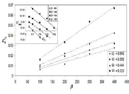
Figure 8: The relationship between $\epsilon_{4}^{C}$ and $\beta$ is extracted by fitting their plots. Shown here are the $\epsilon_{4}^{C}$ vs $\beta$ for $4$ supersaturations, $\Omega=0.666$, $\Omega=0.555$, $\Omega=0.444$, $\Omega=0.333$. Inset: Interpolation of $\epsilon_{4}^{C}$ is extrapolated by fitting measured values for $U_{amp}\rightarrow 0$ for $\Omega=0.444$.

A linear relationship between $\epsilon_{4}^{C}$ and $\beta$ is found for each of the supersaturations studied. These linear relationships are plotted in Figure 8 for the alloy compositions of $C_{o}=0.04,0.05,0.06,0.07$. Figure 8 thus predicts that

$$\epsilon_{4}^{C}=A_{C_{o}}\beta$$ (16)

where the fitting parameter $A_{C_{o}}$ has values of $A_{0.04}=6.84\cdot 10^{-5}$,$A_{0.05}=8.33\cdot 10^{-5}$,$A_{0.06}=10.68\cdot 10^{-5}$ and $A_{0.07}=16.98\cdot 10^{-5}$ for the supersaturations studied.

VI.3 Critical Tip Radii at the Transition Point

The competing anisotropic effects controlling morphology cancel when all correction terms that are dependent on the interface normal angle ($\theta$) in the interfacial equilibrium composition ( $C_{b}^{int}=C_{b}^{eq}-\Delta C_{capillarity}(1+15\epsilon_{4}f(\theta))-\Delta C_{elastic}(1-\epsilon_{e}h(\theta))$ ) exactly cancel. Here $\Delta C_{capillarity}$ and $\Delta C_{elastic}$ are the isotropic corrections to interfacial equilibrium composition and $\epsilon_{4}$ and $\epsilon_{e}$ represent the strength of the surface energy and elastic energy anisotropies. Assuming a linear fourier expansion with a 4-fold symmetry in both $f(\theta)$ and $h(\theta)$ (ie. $cos(4\theta)$) the terms in the interface solute correction can be grouped by order of the fourier expansion.

$$C_{b}^{int}=C_{b}^{eq}-(\Delta C_{capillarity}+\Delta C_{elastic})$$

$$-\left(\epsilon_{surf}-\epsilon_{ele}\right)cos(4\theta)$$ (17)

where $\epsilon_{surf}=15\epsilon_{4}\Delta C_{capillarity}\kappa$ and $\epsilon_{ele}=\epsilon_{e}\Delta C_{elastic}$ are the relative anisotropic strengths of the surface energy correction and the elastic energy correction respectively. The factor of $15$ in the capillarity term comes from the stiffness of the capillarity, $d_{o}(\vec{n})=d_{o}(1+15\epsilon_{4}cos(4\theta))$. The elastic anisotropy strength, $\epsilon_{e}$, is linked to the strength of the elastic anisotropy through $\beta$ and is derived below (see Equation 21).

For an isotropic morphology to emerge the coefficient of $\cos(\theta)$ in Equation 17 is required to vanish, ie.

$$\epsilon_{surf}-\epsilon_{ele}=0$$ (18)

In Equation 17 the capillary term ($\Delta C_{capillary}$) contains a curvature correction, while the elastic term ($\Delta C_{elastic}$) does not. When these terms balance each other a curvature $\kappa$ is selected, which will be associated with a critical radius $R_{trans}^{C}$ (ie. $\kappa_{c}=1/R_{trans}^{C}$). This is determined next.

The capillarity correction is $\Delta C_{capillarity}=(1-k)d_{o}C_{b}^{eq}$, which is used to calculate $\epsilon_{surf}$ as

$$\epsilon_{surf}=15C_{b}^{o}(1-k)d_{o}\epsilon_{4}\kappa$$ (19)

The total elastic correction for cubic coefficients is defined by Equation 5 as $\Delta C_{elastic}=\frac{1}{2}\frac{Z_{1}}{1-k}=\frac{1}{4}\frac{C_{11}+C_{12}}{1-k}\epsilon^{*2}(1-\frac{\epsilon_{xx}+\epsilon_{yy}}{\epsilon^{*}})$. In the absence of elastic anisotropy the strain trace ($\epsilon_{xx}+\epsilon_{yy}$) is zero and therefore

$$\Delta C_{elastic}=\frac{1}{4}\frac{C_{11}+C_{12}}{1-k}\epsilon^{*2}$$ (20)

$\epsilon_{ele}$ is calculated by consideration of the anisotropy in the strain field by substituting Equation 14 for $\epsilon_{xx}+\epsilon_{yy}$, giving

$$1-\frac{\epsilon_{xx}+\epsilon_{yy}}{\epsilon^{*}}=1-\epsilon_{e}cos(4\theta)$$ (21)

where $\epsilon_{e}=\frac{U_{amp}}{\epsilon^{*}}$ and $U_{amp}$ is defined by Equation 15. This results in $\epsilon_{ele}$ becoming

$$\epsilon_{ele}=\frac{1}{8(1-k)}\frac{C_{11}+C_{12}}{C_{11}+\beta}\beta\epsilon^{*2}$$ (22)

Substituting Equations 19 and 22 into Equation 18, the critical radius of curvature required to maintain isotropic conditions is given by,

$$R_{trans}^{C}=120(1-k)^{2}C_{o}^{l}d_{o}\frac{(C_{11}+\beta)}{\epsilon^{*2}(C_{11}+C_{12})}\frac{\epsilon_{4}^{C}}{\beta}$$ (23)

A fit to a selected critical radii is attained by substituting the fitted equation for the critical surface anisotropy coefficient (Equation 16) and by choosing a reference point of $\beta=0$. This results in a relationship for the magnitude of the $\beta=0$ transition radius that depends on concentration through $A_{C_{o}}$ given as,

$$R_{trans}=\frac{120(1-k)^{2}(C_{11})C_{o}^{l}d_{o}}{(C_{11}+C_{12})\epsilon^{*2}}A_{C_{o}}$$ (24)

The next subsection discusses a separate method by which this radius is estimated without the need for measured values of $A_{C_{o}}$.

VI.4 Calculation of the Transition Tip Radius using Linear Stability Approximation

In the previous section a selected precipitate radius is derived based on the interpolated values for the critical surface energy anisotropy. However, this method relates $\epsilon_{4}^{C}$ to $\beta$ only once the value of $A_{C_{o}}$ is measured. A method to approximate the selected radius by theoretical consideration of the Mullins-Sekerka linear stability analysis on an isotropic particle is now shown.

Mullins and Sekerka in 1963 [25, 21] predicted a critical particle size $R^{*}_{k=2}=11R^{*}$ ($R^{*}=\frac{2d_{o}}{\Omega}$, $k$ is the instability mode and $\Omega$ is the supersaturation) after which the particle interface becomes unstable. A particle at the transition point in our study can be considered to behave similarly to an isotropic particle in a supercooled matrix and the tip’s radius of curvature is assumed to be proportional to this critical radius. Here the supersaturation of the precipitate under elastic strain is modified by the elasticity according to $\Omega_{el}=\frac{C_{b}-C_{o}}{(1-k)C_{b}}$, where $C_{b}$ is the equilibrium interface composition modified due to elasticity by Equation 5. This supersaturation is used in the linear stability analysis result to predict a minimum critical radius of,

$$R_{MS}=22\frac{d_{o}}{\Omega_{el}}$$ (25)

A comparison of this instability radius with the fitted radius of equation 24 shows excellent linear agreement as shown in figure 9.

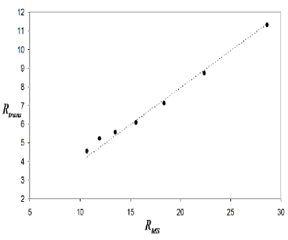
Figure 9: The fitted critical tip radius for isotropic growth, from equation 24, vs the onset Mullins-Sekerka wavelength for seven different supersaturations.

Equation 24 is calculated such that $C_{11}+\beta\rightarrow C_{11}$ in Equation 23. The $\beta$ dependence of $R_{trans}^{C}$ is introduced into Equation 25 through its relationship to $\epsilon_{e}$ by the term $\frac{1}{C_{11}+\beta}$. The final result for the critical selected radius as a function of $\beta$ and $\Omega_{el}$ is

$$R^{MS}_{trans}=\frac{44}{5}\frac{d_{o}}{\Omega_{el}}(1+\frac{\beta}{C_{11}})$$ (26)

VI.5 Calculation of the Critical Transition Point

With the scale of the critical tip radius determined by linear stability theory as a function of supersaturation, the required measurement of the relationship between $\epsilon_{4}^{C}$ and $\beta$ can be eliminated in Equation 23. This is done by substituting the linear stability prediction of the critical radius (Equation 26) into the equation for the selected transition radius (Equation 23). The resulting relationship is solved for the critical surface energy anisotropy pre-factor ($\epsilon_{4}^{C}$). This relationship is

$$\epsilon_{4}^{C}=\frac{11}{150}\frac{C_{11}+C_{12}}{(1-k)^{2}(C_{11}+\beta)C_{o}^{l}\Omega_{el}}\epsilon^{*2}\beta(1+\frac{\beta}{C_{11}})$$ (27)

Equation 27 defines a morphological transition line as a function of supersaturation ($\Omega$), elastic anisotropy ($\beta$) and the anisotropy of the capillarity ($\epsilon_{4}$). The transition lines for $\Omega_{el}=0.606,0.479,0.353,0.226$ are plotted in figure 10. Precipitates grown above the transition line will grow in the [10] directions while growth for conditions below the line will grow along [11] directions. Some morphologies are overplotted above and below the transition line for $\Omega=0.606$ in figure 11 to further illustrate the utility of Equation 27.

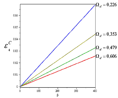
Figure 10: The critical transition points from equation 27. Above the line the precipitates prefer to grow in directions that minimize the surface energy [10], and below the directions which minimize the elastic energy [11]. Transition lines for different $\Omega_{el}$ are plotted. Colour Online.

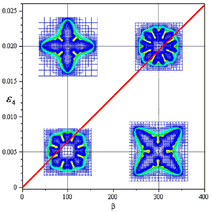
Figure 11: The critical transition line from equation 27. Above the line the precipitates prefer to grow in directions that minimize the surface energy [10], and below the directions which minimize the elastic energy [11]. The curve is plotted vs beta for $C_{o}=0.04$($\Omega_{el}=0.606$). Overplotted are 4 simulations corresponding to different values of $\epsilon_{4}$ and $\beta$. The plotted line represents the value of $\epsilon_{4}^{C}$, the transition point where anisotropies cancel out. Colour Online.

VII Summary

We have introduced a phase-field model for the study of the morphological development of elastically stressed solid state precipitates. We considered particles that have coherent interfaces and are under elastic self stress by a lattice mismatch eigenstrain. We used a new finite difference based adaptive mesh refinement algorithm to solve the phase-field and strain relaxation equations thereby allowing for very rapid solution times. By investigating the effects of supersaturation, elastic anisotropy in the elastic tensor and anisotropy in the capillarity we developed a scaling relationship to predict which anisotropy will be dominant in the morphological evolution of the precipitate. It is interesting note is the effect of supersaturation on the selected precipitate morphology and growth directions.

We would like to thank the National Science and Engineering Research Council of Canada (NSERC) for financial support and SHARC-NET for supercomputing support.

Appendix A Cubic Elastic Free Energy Coefficients

In the generalized elastic portion of the phase field free energy, as described by equation 4 $f_{el}={\it Z_{3}}\left(g_{3}(\phi)\right)^{3}+{\it Z_{2}}\left(g_{3}\left(\phi\right)\right)^{2}+{\it Z_{1}}g_{3}(\phi)+{\it Z_{0}}$, several unknown terms $Z_{3}$, $Z_{2}$, $Z_{1}$ and $Z_{0}$ are introduced. These coeffiecients are dependent on the particular values of the elastic modulus tensor in either of the precipitate or matrix phases. Presented here are the explicit forms for these functions for two sided cubic modula and a hydrostatic elastic eigenstrain of the form,

$$\epsilon^{*}_{ij}=\left|\begin{array}[]{ccc}\epsilon^{*}&0\\ 0&\epsilon^{*}\end{array}\right|.$$

The zeroth order component($Z_{0}$) has no dependence on the phase at all and is calculated to be

$$Z_{0}=\frac{1}{4}(C1_{11}+C2_{11})(\epsilon_{xx}-\frac{\epsilon^{*}}{2})^{2}$$

$$+\frac{1}{4}(C1_{11}+C2_{11})(\epsilon_{yy}-\frac{\epsilon^{*}}{2})^{2}$$

$$+\frac{1}{2}(C1_{12}+C2_{12})(\epsilon_{xx}-\frac{\epsilon^{*}}{2})(\epsilon_{yy}-\frac{\epsilon^{*}}{2})$$

$$+(C1_{44}+C2_{44})\epsilon_{xy}^{2}$$ (28)

This pre-factor has no dependence of phase (nor concentration) and therefore it does not appear in either the phase mobility equation (equation 6) or the chemical diffusion equation (Equation 7) since the growth kinetics are dependent on differences of energy. It does however appear in the static elasticity equation (Equation 8).

The first order component is the most prominent term in the model equations and is calculated to be

$$Z_{1}=\frac{1}{8}(3(C1_{11}+C1_{12})+C2_{11}+C2_{12})\epsilon^{*2}$$

$$-\frac{1}{2}(C1_{11}+C1_{12})(\epsilon_{xx}+\epsilon_{yy})\epsilon^{*}$$

$$+\frac{1}{4}(C1_{11}-C2_{11})(\epsilon_{xx}^{2}+\epsilon_{yy}^{2})$$

$$+\frac{1}{2}(C1_{12}-C2_{12})\epsilon_{xx}\epsilon_{yy}$$

$$+(C1_{44}-C2_{44})\epsilon_{xy}^{2}$$ (29)

The second order coefficient to the elastic energy in terms of the phase is calculated to be

$$Z_{2}=\frac{1}{8}(3(C1_{11}+C1_{12})-(C2_{11}+C2_{12}))\epsilon^{*2}$$

$$+\frac{1}{4}(C2_{11}+C2_{12}-C1_{11}-C1_{12})(\epsilon_{xx}+\epsilon_{yy})\epsilon^{*}$$ (30)

and in the presence of equal elastic coefficients this term becomes a constant.

The third order component is calculated to be

$$Z_{3}=\frac{1}{8}(C1_{11}-C2_{11}+C1_{12}-C2_{12})\epsilon^{*2}$$ (31)

and has no dependence on the dynamic strain field. In the presence of equal elastic coefficients this term vanishes completely.

References

- [1] Athreya B, Goldenfeld N, Dantzig J, Greenwood M, and Provatas N. Physical Review E, 76:056706, 2007.
- [2] Echebarria B, Folch R, Karma A, and Plapp M. Physical Review E, 70:061604, 2004.
- [3] Morin B, Elder K R, Sutton M, and Grant M. Phys Rev Lett, 75:2156, 1995.
- [4] W.J. Boettinger, J.A. Warren, C. Beckermann, and A. Karma. Annu Rev. Mater. Res., 32:163, 2002.
- [5] Tong C, Greenwood M, and Provatas N. Physical Review B, 77:064112, 2008.
- [6] Eshelby J D. Proc Roy Soc London A, 241:376, 1957.
- [7] Yeon D, Cha P, Kim J, Grant M, and Yoon J. Modelling Simul. Mater. Sci. Eng., 13:031609, 2005.
- [8] Kessler DA, Koplik J, and Levine H. Adv Phys, 37:255, 1988.
- [9] Ben-Jacob E, Goldenfeld N, Langer JS, and Schon G. Phys Rev A, 29:330, 1984.
- [10] Meiron D I. Phys Rev A, 33:2704, 1986.
- [11] Steinbach I and Apel M. Physica D - Nonlinear Phenomena, 217:153, 2006.
- [12] Hoyt J J, Asta M, and Karma A. Matls. Sci. Eng., 41:121, 2003.
- [13] Jou H J, Leo P H, and Lowengrub J S. J Comp Phys, 131:109, 1997.
- [14] Laraia V J, Johnson W C, and Voorhees P W. J Mater Res, 3:257, 1988.
- [15] Malcolm JA and Purdy GR. Trans Metall Soc AIME, 239:1391, 1967.
- [16] Zhu J.Z., Wang T, Ardell AJ, Zhou SH, Liu ZK, and Chen LQ. Acta Mater, 52:2837, 2004.
- [17] Aguenaou K, Muller J, and Grant M. Philos Mag B, 78:103, 1998.
- [18] Kassner K, Misbah C, Muller J, Kappey J, and Kohlert P. J. Cryst. Growth, 225:289, 2001.
- [19] Kassner K, Misbah C, Muller J, Kappey J, and Kohlert P. Phys Rev E, 63:036117, 2001.
- [20] A. Karma and W.-J. Rappel. Phys. Rev. E, 53:3017, 1996.
- [21] J.S. Langer. Rev. Mod. Phys., 52:1, 1980.
- [22] Greenwood M. PhD Thesis - In Submission, 2008.
- [23] Haataja M, Muller J, Rutenberg A D, and Grant M. Phys Rev B, 65:035401, 2001.
- [24] M.Haataja, J.Mahon, N.Provatas, and Leonard. , 2004.
- [25] W. W. Mullins and R. F. Sekerka. J. Appl. Phys., 34:323, 1963.
- [26] Provatas N, Greenwood M, Athreya B, Goldenfeld N, and Dantzig J. International Journal of Modern Physics, 19:4525, 2005.
- [27] Provatas N, Wang Q, Haataja, and Grant M. Physical Review Letters, 91:155502, 2003.
- [28] N. Provatas, N. Goldenfeld, J. Dantzig, J.C. LaCombe, A. Lupulescu, M.B. Koss, M.E. Glicksman, and R. Almgren. Phys. Rev. Let., 82:4496, 1999.
- [29] Ru C Q. Acta Mechanica, 160:219, 2003.
- [30] Hazhimali T, Karma A Gonzales F, and Rappaz M. Nature Materials, 5:660, 2006.
- [31] Wang Y U, Jin Y M, and Khachaturyan A G. Appl Phys Lett, 80:4513, 2002.
- [32] Wang Y U, Jin Y M, and Khachaturyan A G. J Appl Phys, 92:1351, 2002.
- [33] Vaithyanathan V, Wolverton C, and Chen L.Q. Acta Mat, 52:2973, 2004.
- [34] Husain S W, Ahmed M S, and Qamar I. Metall. Mater. Trans. A, 30A:1529, 1999.
- [35] Voorhees P W, McFadden G B, and Johnson W C. Acta Metall Mater, 40:1979, 1992.
- [36] Dong-Hee Yeon, Pil-Ryung Cha, Ji-Hee Kim, Martin Grant, and Jong-Kyu Yoon. Model and Simul in Mat Sci and Eng, 13:299, 2005.
- [37] Yoo Y.S. Scr Mater, 53:81, 2005.