Osmotically driven flows in microchannels separated by a semipermeable membrane

Abstract

We perform experimental investigations of osmotically driven flows in artificial microchannels by studying the dynamics and structure of the front of a sugar solution traveling in $200\,\mu$m wide and $50-200\,\mu$m deep microchannels. We find that the sugar front travels with constant speed, and that this speed is proportional to the concentration of the sugar solution and inversely proportional to the depth of the channel. We propose a theoretical model, which, in the limit of low axial flow resistance, predicts that the sugar front indeed should travel with a constant velocity. The model also predicts an inverse relationship between the depth of the channel and the speed and a linear relation between the sugar concentration and the speed. We thus find good agreement between the experimental results and the predictions of the model. Our motivation for studying osmotically driven flows is that they are believed to be responsible for the translocation of sugar in plants through the phloem sieve element cells. Also, we suggest that osmotic elements can act as integrated pumps with no movable parts in lab-on-a-chip systems.

I Introduction

Osmotically driven flows are believed to be responsible for the translocation of sugar in plants, a process that takes place in the phloem sieve element cells Taiz and Zeiger (2002). These cells form a micro-fluidic network which spans the entire length of the plant measuring from 10 $\mu$m in diameter in small plants to 100 $\mu$m in diameter in large trees Taiz and Zeiger (2002). The mechanism driving these flows is believed to be the osmotic pressures that build up relative to the neighboring water-filled tissue in response to loading and unloading of sugar into and out of the phloem cells in different parts of the plant Taiz and Zeiger (2002). This mechanism, collectively called the pressure-flow hypothesis, is much more efficient than diffusion, since the osmotic pressure difference caused by a difference in sugar concentration creates a bulk flow directed from large concentrations to small concentrations, in accordance with the basic needs of the plant.

Experimental verification of flow rates in living plants is difficult Knoblauch and van Bel (1998), and the experimental evidence on artificial systems backing the pressure-flow hypothesis is scarce and consists solely of results obtained with centimetric sized setups Eschrich et al. (1972); Lang (1973); Jensen et al. (Submitted, 2008). However, many theoretical and numerical studies of the sugar translocation in plants have used the pressure-flow hypothesis Thompson and Holbrook (2003a, b); Hölttä (2006) with good results. To verify that these results are indeed valid, we believe that it is of fundamental importance to conduct a systematic survey of osmotically driven flows at the micrometer scale. Finally, osmotic flows in microchannels can potentially act as micropumps with no movable parts in much the same way as the osmotic pills developed by Shire Laboratories and pioneered by F. Theeuwes Theeuwes (1975). Also, there is a direct analogy between osmotically driven flows powered by concentration gradients, and electroosmotically driven flows in electrolytes Brask et al. (2005); Gregersen et al. (2007) powered by electrical potential gradients.

II Experimental setup

II.1 Chip design and fabrication

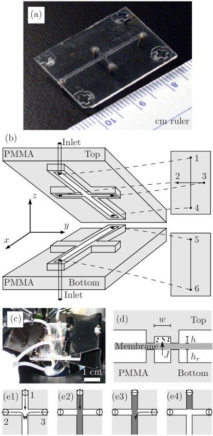
Figure 1: (a) Picture of the top part (upside down) of the chip showing the elevated channel and the four brass inlet tubes (pointing down). The crosses in the four corners were used for alignment. (b) Schematics of the two PMMA layers (gray) showing the elevated channels (white) facing each other. All six inlet positions (black dots) are marked, but for clarity only two brass tubes are shown. (c) Picture of the setup assembled. (d) Schematic cross-section closeup of the two PMMA layers (gray) clamped together with the semipermeable membrane (dark gray) in between. The sugar in the upper channel (black dots) and the water influx $J$ from the lower channel (arrow) are also marked. (e1)-(e4) Valve settings (circles) and cross-flow flushing procedure (arrows) for creating a sharp front in the top channel between the sugar/dye solution (dark gray) and the pure water (white). See details in the text.

To study osmotically driven flows in microchannels, we have designed and fabricated a microfluidic system consisting of two layers of 1.5 mm thick polymethyl methacrylate (PMMA) separated by a semipermeable membrane (Spectra/Por Biotech Cellulose Ester dialysis membrane, MWCO 3.5 kDa, thickness $\sim 40\,\mu$m), as shown in Fig. 1(a)-(d). Channels of length 27 mm, width 200 $\mu$m and depth $50-200\,\mu$m were milled in the two PMMA layers by use of a MiniMill/Pro3 milling machine Geschke (2004); Bundgaard et al. (2007). The top channel contains partly the sugar solution, and partly pure water, while the bottom channel always contains only pure water. To facilitate the production of a steep concentration gradient by cross-flows, a 200 $\mu$m wide cross-channel was milled in the upper PMMA layer perpendicular to and bi-secting the main channel. Inlets were produced by drilling $800$ $\mu$m diameter holes through the wafer and inserting brass tubes into these. By removing the surrounding material, the channel walls in both the top and bottom layers acquired a height of $100\,\mu$m and a width of $150\,\mu$m. After assembly, the two PMMA layers were positioned such that the main channels in either layer were facing each other. Thus, when clamping the two layers together using two $30\,$mm paper clamps, the membrane acted as a seal, stopping any undesired leaks from the channels as long as the applied pressure did not exceed approximately 1 bar.

II.2 Measurement setup and procedures

Table 1: List of parameters in alphabetic order after the symbol.

Parameter	Symbol	Value and/or unit
Initial concentration	$c_{0}$	mol/L
Diffusion constant	$D$	m2/s
Height of channel	$h$	$50,100,200$ $\mu$m
Height of reservoir	$h_{r}$	$200$ $\mu$m
Flux across membrane	$J$	m/s
Length of channel	$L$	27 mm
Membrane permeability	$L_{p}$	$1.8\,$ pm/(Pa s)
Diffusion length	$l_{D}$	m
Münch number	$M$
Hydrostatic pressure	$p$	Pa
Péclet number, local	Pé
Péclet number, global	Pég
Gas constant	$R$	$8310\,$Pa L/(K mol)
Position of sugar front	$s$
Absolute temperature	$T$	K
Time	$t$	s
$x$-velocity of sugar front	$U$	m/s
Mean $x$-velocity of sugar front	$u$	m/s
Volume behind sugar front	$V$	m3
Width of channel	$w$	200 $\mu$m
Width of sugar front	$w_{f}$	m
Cartesian coordinates	$x,y,z$	m
Osmotic coefficients:
Dextran ($T=293\,$K)	$\alpha$	41, see Ref. Jensen et al. (Submitted, 2008)
Sucrose ($T=293\,$K)	$\alpha$	1, see Ref. Michel (1972)
Viscosity	$\eta$	Pa s
Position of sugar front	$\lambda$	m
Position of initial sugar front	$\lambda_{0}$	13.5 mm
Osmotic pressure	$\Pi$	Pa

In our setup, the osmotic pressure pushes water from the lower channel, through the membrane, and into the sugar-rich part of the upper channel. This displaces the solution along the upper channel thus generating a flow there. To measure this flow inside the upper channel, particle and dye tracking were used. In both cases inlets 1, 2, 3 and 5 (see Fig. 1) were connected via silicone tubing (inner diameter 0.5 mm) to disposable syringes. Syringes 2, 3 and 5 was filled with demineralised water and syringe 1 was filled with a solution of sugar (sucrose or dextran (mol. weight: 17.5 kDa, Sigma-Aldrigde, type D4624)) and 5 $\%$ volume red dye (Flachsmann Scandinavia, Red Fruit Dye, type 123000) in the dye tracking experiments and 0.05 $\%$ volume sulfate modified $1$ $\mu$m polystyrene beads (Sigma Aldrigde, L9650-1ML) in the particle tracking experiments. Inlets 4 and 6 were connected to the same water bath to minimize the hydrostatic pressure difference between the two sides of the membrane.

When conducting both dye tracking and particle tracking experiments, the initialization procedure shown in Fig. 1(e1)-(e4) was used: First (e1), inlet valves 1, 2 and 3 were opened and all channels were flushed thoroughly with pure water (white) to remove any air bubbles and other impurities. Second (e2), after closing inlets 2 and 3 a sugar solution (dark gray) was injected through inlet 1 filling the main channel in the upper layer. Third (e3), inlet 1 was closed and water was carefully pumped through inlet 2 to produce a sharp concentration front at the cross, as shown in Fig. 1(e4) and 2(b).

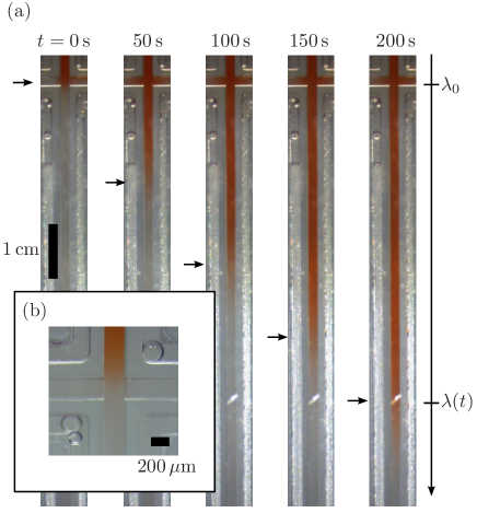
Figure 2: (a): Images showing the sugar front moving in the $200\,\mu$m$\times 200\,\mu$m channel. The time between each image is 50 s. The arrows indicate the position of the sugar front as it moves down along the channel. (b): Closeup of the cross junction just after a sharp sugar/water interface has been created.

II.2.1 Sugar front motion recorded by dye tracking

The motion of the sugar front in the upper channel was recorded by taking pictures of the channel in 10 s intervals using a Leica MZ 16 microscope. This yielded images as those displayed in Fig. 2(a), clearly showing a front (marked by arrows) of the sugar/dye solution moving along the channel. To obtain the position $\lambda(t)$ of the sugar front as a function of time $t$, the distance from the initial front position $\lambda_{0}$ to the current position $\lambda(t)$ was measured using ImageJ software. The position of the sugar front was taken to be at the end of the highly saturated dark region. In this way, the position of the front could be measured at each time step with an accuracy of $\pm$200 $\mu$m. As verified in earlier works Eschrich et al. (1972); Jensen et al. (Submitted, 2008), we assumed that the sugar and dye traveled together, which is reasonable since the Péclet number is $P\acute{e}\sim 10$ (see Section IV). We only applied the dye tracking method on the $200$ $\mu$m deep channel, since the $100$ $\mu$m and $50$ $\mu$m deep channels were too shallow for sufficient scattering of red light by the solution to get a clear view of the front.

II.2.2 Sugar front motion recorded by use of particle tracking

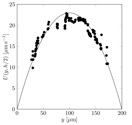
Figure 3: Velocity profile $U(y,h/2)$ obtained in the center plane across the $200\,\mu$m$\times 200\,\mu$m channel. The solid black line is a fit to Eq. (2).

The flow velocity inside the upper channel was recorded by tracking the motion of $1$ $\mu$m beads in the water $3$ mm ahead of the initial sugar front position. Images were recorded every $200-1000$ ms using a Unibrain Fire-i400 1394 digital camera attached to a Nikon Diaphot microscope with the focal plane at $h/2$. From the images we extracted velocity profiles such as the one shown in Fig. 3. At the point of observation well ahead of the front, the flow behaves as if it were pressure driven. In that case the laminar flow profile $U$ in the rectangular straight top channel of height $h$, width $w$, and length $L$ is given by the expression Bruus (2008)

$$U(y,z)=\frac{4h^{2}\Delta p}{\pi^{3}\eta L}\sum_{n,\text{odd}}^{\infty}\frac{1}{n^{3}}\left[1-\frac{\cosh\left(n\pi\frac{y}{h}\right)}{\cosh\left(n\pi\frac{w}{2h}\right)}\right]\sin\left(n\pi\frac{z}{h}\right).$$ (1)

At the center of the channel, $z=h/2$, this simplifies to

$$U(y,h/2)=\frac{4h^{2}\Delta p}{\pi^{3}\eta L}\sum_{n,\text{odd}}^{\infty}\frac{(-1)^{n}}{n^{3}}\left[1-\frac{\cosh\left(n\pi\frac{y}{h}\right)}{\cosh\left(n\pi\frac{w}{2h}\right)}\right].$$ (2)

To determine the pre-factor, we fit Eq. (2) to our data points obtained by particle tracking. The average velocity $u$ inside the channel is then

$$u=\frac{h^{2}\Delta p}{12\eta L}\left[1-\sum_{n,\text{odd}}\frac{1}{n^{5}}\frac{192}{\pi^{5}}\frac{h}{w}\tanh\left(n\pi\frac{w}{2h}\right)\right].$$ (3)

III Experimental results

III.1 Dye tracking

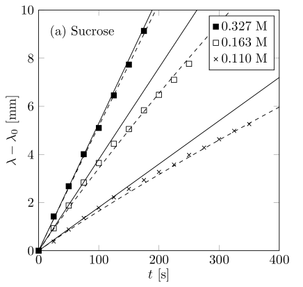
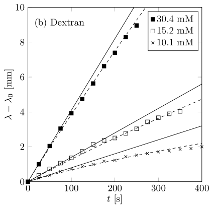
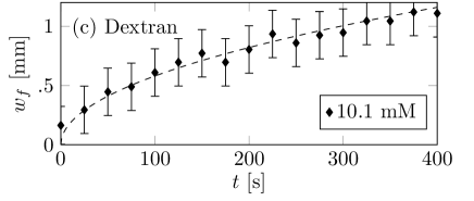
Figure 4: Measured position $\lambda$ of the sugar front as a function of time $t$ in the $200\,\mu$m$\times 200\,\mu$m channel for various concentrations of (a) sucrose and (b) dextran. The solid black lines are linear fits for $0\;$s$\,<\,t\,<100\,$s. The dashed lines are fits to Eq. (16). (c) The width $w_{f}$ of the sugar front as a function of time for the 10.1 mM dextran experiment. The dashed black line is a fit to $\left(2Dt\right)^{1/2}$ with $D=1.7\times 10^{-9}\,$m${}^{2}\,$s^-1.

Figure 4 shows the position of the sugar front in the $200$ $\mu$m deep channel as a function of time obtained by dye tracking. The data sets correspond to different concentrations of sucrose and dextran as indicated in the legends. Initially, the sugar front moves with constant speed, but then it gradually decreases, more so for low than high concentrations. The solid black lines are linear fits for the first 100 s giving the initial velocity of the front. In Fig. 4(c) the width of the sugar front for the 10.1 mM dextran experiment is shown along with a fit to $\left(2Dt\right)^{1/2}$ showing that the sugar front broadens by molecular diffusion.

III.2 Particle tracking

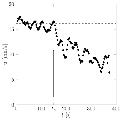
Figure 5: The average flow velocity $u$ in the 200 $\mu$m deep channel as a function of time $t$ measured 3 mm ahead of the initial front position. At $t_{c}\simeq 150\,$s the sugar front begins to reach the observation point, and the velocity decreases rapidly. For $t>t_{c}$, the velocity was not determined accurately.

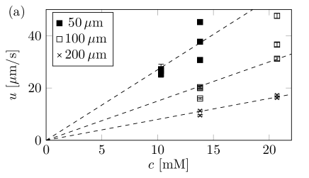
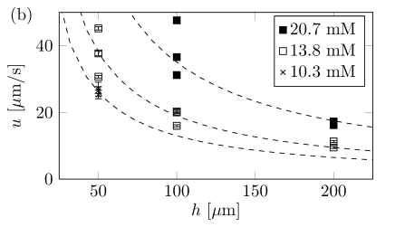
Figure 6: Front velocity $u$ obtained by particle tracking. (a) The velocity $u$ plotted against dextran concentration $c_{0}$. The dashed lines are fits to $c$ provided as guides to the eye. (b) The velocity $u$ plotted against channel depth $h$. The dashed lines are fits to $1/h$ provided as guides to the eye.

Figure 5 shows the velocity as a function of time obtained by particle tracking in a $200\,\mu$m$\times 200\,\mu$m channel. For the first $150$ s the velocity is approximately constant after which it starts decreasing as the sugar front passes the point of observation. We interpret the mean value of the initial plateau of the velocity graph as the speed of the sugar front. Figs. 6(a) and (b) shows the velocity of the sugar front as a function of dextran concentration and of channel depth obtained in this way.

IV Theoretical analysis

When modeling the flow inside the channel, we use an approach similar to that of Eschrich et al. Eschrich et al. (1972). They introduced a 1D model with no axial flow resistance and zero diffusivity in a setting very similar to ours. To formalize this, we consider the two most important non-dimensional numbers in the experiments: the Münch number $M$ Jensen et al. (Submitted, 2008) and the Péclet number $P\acute{e}$ Bruus (2008). These numbers characterize the ratio of axial to membrane flow resistance and axially convective to diffusive fluxes respectively. In our experiments

$$M=\frac{\eta L^{2}L_{p}}{h^{3}}\sim 10^{-6},$$ (4)

and

$$P\acute{e}=\frac{w_{f}u}{D}\sim 10.$$ (5)

Here $\eta$ is the viscosity (typically $1.5$ mPa s), $w_{f}$ is the front width (typically $500$ $\mu$m), and $D$ the molecular diffusivity of sugar (typically $10^{-10}$ m²s^-1 for sucrose and the dye and $10^{-11}$ m²s^-1 for dextran)

IV.1 Equation of motion

Since $M\ll 1$ and $Pe\gg 1$, we shall neglect the axial flow resistance and the diffusion of the sugar in our analysis. In this way, let $\lambda(t)$ denote the position of the sugar/dye front in the upper channel, and let $V$ denote the volume behind the front. The flux $J$ of water across the membrane from the lower to the upper channel, see Fig. 1(d), is given by

$$J=L_{p}\left(\Delta p+\Delta\Pi\right)\simeq L_{p}\alpha RTc,$$ (6)

where $L_{p}$ is the membrane permeability, $\Delta p$ the hydrostatic and $\Delta\Pi$ the osmotic pressure difference across the membrane. In our experiments $\Delta p=0$, and from the van ’t Hoff relation follows $\Delta\Pi\simeq\alpha RTc$, where $\alpha$ is the osmotic coefficient, $R$ is the gas constant, $T$ is the absolute temperature, and $c$ is the concentration of sugar molecules. Since the concentration is independent of $x$ behind the front and zero ahead of it, $J$ is also independent of $x$. By the conservation of sugar this allows us to write the concentration as

$$c(x,t)=\begin{cases}c_{0}\frac{\lambda_{0}}{\lambda(t)}&x\leq\lambda(t),\\ 0&x\geq\lambda(t).\\ \end{cases}$$ (7)

Moreover, the rate of change of the expanding volume $V$ behind the front can be related to $J$ as

$$\frac{\mathrm{d}V}{\mathrm{d}t} = w\int_{0}^{L}J(x)dx$$ (8)

$$= wL_{p}\alpha RTc_{0}\frac{\lambda_{0}}{\lambda(t)}\int_{0}^{\lambda(t)}\mathrm{d}x$$

$$= w\lambda_{0}L_{p}\alpha RTc_{0}.$$

However, we also have that

$$\frac{\mathrm{d}V}{\mathrm{d}t}=hw\frac{\mathrm{d}\lambda(t)}{\mathrm{d}t},$$ (9)

which implies together with Eq. (8) that

$$\lambda(t)=\lambda_{0}+\frac{\lambda_{0}}{h}L_{p}\alpha RTc_{0}t=\lambda_{0}+ut,$$ (10)

where the velocity $u$ of the front is given by

$$u=\frac{\lambda_{0}}{h}L_{p}\alpha RTc_{0}.$$ (11)

IV.2 Corrections to the equation of motion

In the previous section, we considered the motion of a sharp sugar front, as given by the stepwise concentration profile in Eq. (7), and found that this moved with constant velocity. However, as can be seen in Fig. 4 the front velocity gradually decreases. To explain this, we observe that in Fig. 2(a) there exist a region of growing size separating the sugar-filled region from the region of pure water. This intermediate region is caused by diffusion and hence denoted the diffusion region. The end point of the sugar region is denoted $\lambda$, while the width of the diffusion region, which is growing in time, is denoted $l_{D}$. Consequently, the concentration profile can be approximated by the following simple three-region model,

$$c(x,t)=\begin{cases}c_{t},&0\leq x\leq\lambda,\\[5.69054pt] c_{t}\left(1-\frac{x-\lambda}{l_{D}}\right),&\lambda\leq x\leq\lambda+l_{D},\\[5.69054pt] 0,&\lambda+l_{D}\leq x\leq L.\\ \end{cases}$$ (12)

Here $l_{D}=(2Dt)^{1/2}$ and $c_{t}=c_{0}\frac{\lambda_{0}}{\lambda+l_{D}/2}$ from conservation of sugar. Using Eqs. (8) and (9) the time derivative of $\lambda$ becomes

$$\frac{\mathrm{d}\lambda}{\mathrm{d}t}=\frac{L_{p}\alpha RTc_{0}\lambda_{0}}{h}\frac{\lambda}{\lambda+l_{D}}.$$ (13)

Rescaling using $\lambda=s\lambda_{0}$ and $t=\tau\frac{\lambda_{0}}{u}$, we get that

$$\frac{\mathrm{d}s}{\mathrm{d}\tau}=\frac{s}{s+\left(\frac{\tau}{P\acute{e}_{g}}\right)^{1/2}},$$ (14)

where we have introduced the global Péclet number

$$P\acute{e}_{g}=\frac{2\lambda_{0}^{2}L_{p}\alpha RTc_{0}}{Dh}=\frac{2\lambda_{0}}{D}u.$$ (15)

Given the experimental conditions, $P\acute{e}_{g}$ is typically of the order $10^{1}-10^{2}$. Thus, for $\left(\frac{\tau}{P\acute{e}_{g}}\right)^{1/2}\ll 1$, Eq. (14) can be solved by an expansion,

$$s=s_{0}+\tau\left(1-\frac{2}{3s_{0}}\left(\frac{\tau}{P\acute{e}_{g}}\right)^{1/2}+\mathcal{O}\left[\left(\frac{\tau}{P\acute{e}_{g}}\right)\right]\right).$$ (16)

The dashed lines in Figs. 4(a) and (b) are fits to Eq. (16), with values of $D$ between $2\times 10^{-7}\,$m${}^{2}\,$s^-1 and $4\times 10^{-9}\,$m${}^{2}\,$s^-1, showing good qualitative agreement between theory and experiment. However, these values of $D$ are 1 to 100 times larger than that obtained in Fig. 4(c) ($1.7\times 10^{-9}\,$m${}^{2}\,$s^-1) indicating a quantitative discrepancy between the experimental data and our model. We suspect that this is due to some accelerated diffusion mechanism occurring at the front, such as Taylor dispersion Taylor (1953); Lee et al. (2008). To resolve this issue, experiments of higher accuracy are required as well as direct tracking of the sugar without using a dye.

V Discussion

V.1 Comparison of theory and experiment

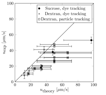
Figure 7: The experimental values of $u$ plotted against the results from Eq. (11).

To compare the experimental data with theory, we have in Fig. 7 plotted the empirically obtained velocities $u_{\rm exp}$ against those predicted by Eq. (11). For nearly all the dextran and sucrose experiments we see a good agreement between experiment and theory, although Eq. (11) systematically overestimates the expected velocities.

We interpret the quantitative disagreement as an indication of a decreasing sugar concentration in the top channel due to diffusion of sugar into the membrane as well as the presence of a low-concentration boundary layer near the membrane, a so-called unstirred layer Pedley (1983).

V.2 Osmotic pumps in lab-on-a-chip systems

Depending on the specific application, flows in lab-on-a-chip systems are conventionally driven by either syringe pumps or by using more advanced techniques such as electronically controlled pressure devices, electro-osmotic pumps Ajdari (2000), evaporation pumps Noblin et al. (2008), or capillary pumps Boudait et al. (2005). Most of these techniques involves the integration of either movable parts or complicated electronics into the lab-on-a-chip device. As an application of our results, we suggest the use of osmotic pumps in lab-on-a-chip systems. This could be done by integrating in the device a region where the channel is in contact through a membrane with a large reservoir containing an osmotically active agent. By using a sufficiently large reservoir, say $1\,$cm³, and a $100\,\mu$m$\times 100\,\mu$m channel with a flow rate of $100\,\mu$m/s it would take more than $10$ days to reduce the reservoir concentration by $50$% and thus decreasing the pumping rate by 50%. We emphasize that such osmotic pumping would be completely steady, even at very low flow rates.

VI Conclusions

We have studied osmotically driven, transient flows in 200 $\mu$m wide and $50-200$ $\mu$m deep microchannels separated by a semipermeable membrane. These flows are generated by the influx of water from the lower channel, through the membrane, into the large sugar concentration placed in one end of the top channel. We have observed that the sugar front in the top channel travels with constant speed, and that this speed is proportional to the concentration of the sugar solution and inversely proportional to the depth of the channel. We propose a theoretical model, which, in the limit of low axial flow resistance, predicts that the sugar front should travel with a constant velocity. The model also predicts an inverse relationship between the depth of the channel and the speed and a linear relation between the sugar concentration and the speed. We compare theory and experiment with good agreement, although the detailed mechanism behind the deceleration of the flow is still unknown. Finally, we suggest that osmotic elements can potentially act as pumps with no movable parts in lab-on-a-chip systems.

VII Acknowledgements

It is a pleasure to thank Emmanuelle Rio, Christophe Clanet, Frederik Bundgaard, Jan Kafka and Oliver Geschke for assistance and advice on chip design and manufacturing. We also thank Alexander Schulz, Michele Holbrook, Maciej Zwieniecki and Howard Stone for many useful discussions of the biological and phycial aspects of osmotically driven flows. This work was supported by the Danish National Research Foundation, Grant No. 74 and by the Materials Research Science and Engineering Center at Harvard University.

References

- Taiz and Zeiger (2002) L. Taiz and E. Zeiger, Plant Physiology (Sinauer Associates, Inc., 2002), 3rd ed.
- Knoblauch and van Bel (1998) M. Knoblauch and A. J. E. van Bel, The Plant Cell 10, 35 (1998).
- Eschrich et al. (1972) W. Eschrich, R. F. Evert, and J. H. Young, Planta (Berl.) 107, 279 (1972).
- Lang (1973) A. Lang, Journal of Experimental Botany 24, 896 (1973).
- Jensen et al. (Submitted, 2008) K. Jensen, E. Rio, R. Hansen, C. Clanet, and T. Bohr, Journal of Fluid Mechanics (Submitted, 2008), eprint arXiv:0810.4021v1.
- Thompson and Holbrook (2003a) M. V. Thompson and N. M. Holbrook, J Theo Biol 220, 419 (2003a).
- Thompson and Holbrook (2003b) M. V. Thompson and N. M. Holbrook, Plant, Cell and Environment 26, 1561 (2003b).
- Hölttä (2006) T. Hölttä, Trees - Structure and Function 20, 67 (2006).
- Theeuwes (1975) F. Theeuwes, J. Pharm. Sci. 64, 1987 (1975).
- Brask et al. (2005) A. Brask, J. Kutter, and H. Bruus, Lab Chip 5, 730 (2005).
- Gregersen et al. (2007) M. Gregersen, L. Olesen, A. Brask, M. Hansen, and H. Bruus, Phys. Rev. E 76, 056305 (2007).
- Geschke (2004) O. Geschke, Microsystem Engineering of Lab-on-a-Chip Devices (Wiley-VCH, 2004).
- Bundgaard et al. (2007) F. Bundgaard, G. Perozziello, and O. Geschke, Proceedings of the Institution of Mechanical Engineers Series C 220, 1625 (2007).
- Michel (1972) B. E. Michel, Plant Physiol. 50, 196 (1972).
- Bruus (2008) H. Bruus, Theoretical Microfluidics (Oxford University Press, 2008).
- Taylor (1953) G. I. Taylor, Proc. Roy. Soc. A 291, 186 (1953).
- Lee et al. (2008) J. Lee, E. Kulla, A. Chauhan, and A. Tripathi, Phys. Fluids 20, 093601 (2008).
- Pedley (1983) T. J. Pedley, Quarterly Review of Biophysics 16, 115 (1983).
- Ajdari (2000) A. Ajdari, Phys. Rev. E 61, R45 (2000).
- Noblin et al. (2008) X. Noblin, L. Mahadevan, I. A. Coomaraswamy, D. A. Weitz, N. M. Holbrook, and M. A. Zwieniecki, PNAS 105, 9140 (2008).
- Boudait et al. (2005) S. Boudait, O. Hansen, H. Bruus, C. Berendsen, N. Bau-Madsen, P. Thomsen, A. Wolff, and J. Jonsmann, Lab Chip 5, 827 (2005).