Encoding information into precipitation structures

Abstract

Material design at submicron scales would be profoundly affected if the formation of precipitation patterns could be easily controlled. It would allow the direct building of bulk structures, in contrast to traditional techniques which consist of removing material in order to create patterns. Here, we discuss an extension of our recent proposal of using electrical currents to control precipitation bands which emerge in the wake of reaction fronts in ${\rm A^{+}+B^{-}\to C}$ reaction-diffusion processes. Our main result, based on simulating the reaction-diffusion-precipitation equations, is that the dynamics of the charged agents can be guided by an appropriately designed time-dependent electric current so that, in addition to the control of the band spacing, the width of the precipitation bands can also be tuned. This makes straightforward the encoding of information into precipitation patterns and, as an amusing example, we demonstrate the feasibility by showing how to encode a musical rhythm.

• Keywords: Pattern formation (Theory), Chemical kinetics, Coarsening processes, Nonlinear dynamics, Kinetic growth processes (Theory)

1 Introduction

Information encoding and material design involves the creation of patterns which, in practice, often means that structures must be produced in a homogeneous media. At submicron range which is the target for downscaling of electronic devices, the control over the desired patterns becomes difficult and, furthermore, the expenses of traditional top-down methods (such as e.g. lithography where material is removed in order to create structures) grow steeply. A possible way out of the difficulties is the so called bottom-up design where one aims at forming structures directly in the bulk. Nature, of course, provides us with illuminating examples of three-dimensional pattern formation at all scales [1, 2]. Among them, there is a much studied class of reaction-diffusion processes yielding precipitation patterns [3], and these processes – suitably planned and controlled – are promising candidates for bottom-up designs [4, 5]. Indeed, there has been a series of attempts to control the emerging patterns by appropriately chosen geometry [6] and boundary conditions [5], or by a combined tuning of the initial and boundary conditions [7, 8]. Unfortunately, the above methods of control are not practical enough, and more flexible approaches are required.

Recently, we introduced a novel method of pattern control [9] based on the use of electric currents for regulating the dynamics of the reaction zones. We showed both theoretically and experimentally that, by controlling the reaction zones, the positions of precipitation bands were predesignable. Here we further develop the theory of the new method and show that, in addition to the control of the spacings of the precipitation bands, it is possible to control the widths of the bands, as well. Thus an extra degree of freedom appears which can be used to encode information. We demonstrate the utility of this extra freedom by encoding rhythmic patterns into precipitation structures.

In order to describe the new features of the control by electric currents, we begin by a brief description of the properties of the all important reaction zones which provide the main input to the precipitation process in the wake of the zone (Sec.2). Next, the effect of time dependent electric currents is described and the mathematical details needed for the simulations of the process are explained (Sec.3). Finally the idea of how to control the width of the precipitation band is introduced and examples of information encoded into the widths are presented (Sec.4).

2 Understanding natural precipitation patterns

The basic idea for the pattern control comes from the observation that precipitation patterns are often formed in the wake of moving reaction fronts [2, 3]. The motion of the front and its reaction dynamics determines where and when the concentration of reaction product crosses a threshold thus inducing precipitation. Consequently, and this is the essence of our proposal, control over the precipitation pattern can be realized by regulating the properties of the reaction fronts. Guiding reaction fronts and tuning the reaction rates in them, however, does not appear to be an easy task. In order to explain how it can be done, we turn to the concrete example of Liesegang patterns [3, 10]. They have been studied for more than a century and a wealth of information has been collected about the properties of the front dynamics underlying this pattern formation.

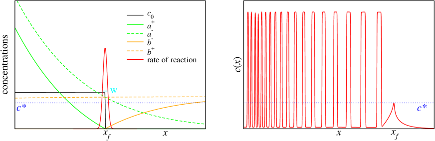
Figure 1: Left panel: Concentration profiles near the reaction zone. Concentrations of the reacting ions ($a^{+},b^{-}$), of the counter ions ($a^{-},b^{+}$), and of the reaction product $c_{0}$ left in the wake of the front are plotted. The reaction zone defined as the region where the rate of $C$ production is significantly different from zero moves diffusively ($x_{f}\sim\sqrt{t}$) and remains well localized during the process. Right panel: Moment of the creation of a band in the phase separation process – the concentration $c$ reaches the threshold value $c^{*}$ at the position of the front, $x_{f}$.

2.1 Properties of a diffusive reaction front

Liesegang patterns are characteristic examples of precipitation structures formed in the wake of moving reaction fronts [11]. The main ingredients are two electrolytes $A\equiv(A^{+},A^{-})$ and $B\equiv(B^{+},B^{-})$ which react with reaction rate $k$ according to the reaction scheme $A^{+}+B^{-}\stackrel{{\scriptstyle k}}{{\rightarrow}}C$. The reaction product $C$ may participate in further reactions but, in the simplest case considered here, it just undergoes a phase separation process resulting in an insoluble precipitate provided the local concentration is above some threshold [12]. In a typical experiment, the electrolytes are initially separated with the inner electrolyte $B$ homogeneously dissolved in a gel column while the outer electrolyte $A$ is kept in an aqueous solution. At time $t=0$, the outer electrolyte brought into contact with the end of the gel column and, since the initial concentration, $a_{0}$, of $A$ is chosen to be much higher than that of $B$ (typically $a_{0}/b_{0}\approx 100$), $A$ invades the gel and a reaction front emerges which advances along the column. The motion of this front and the amount of reaction product $C$ left behind the front are clearly important factors since they determine the input for the precipitation processes.

The main features of the reaction front (see left panel of Fig. 1) are well known [13, 14] and can be summarized in the following three points:

(i)   The front moves diffusively. Its position $x_{f}$ is given by $x_{f}(t)=\sqrt{2D_{f}t}$ where the diffusion coefficient $D_{f}$ is determined by the initial concentrations ($a_{0}$, $b_{0}$) and by the diffusion coefficients of the reagents.

(ii) The front is localized. Although the width w of the front is slowly increasing with time $(\hbox{w}\sim t^{1/6})$, it is always much smaller than the diffusive lengthscales $(\sim t^{1/2})$ present in the problem. Furthermore, the width becomes negligible for fast reactions $(\hbox{w}\sim 1/k^{1/3})$.

(iii) The concentration $c_{0}$ of the reaction product, $C$, left in the wake of the front is constant with a value depending on the initial concentrations and on the diffusion constants of the reagents.

Clearly, all these properties are important: (i) tells the location of the front, (ii) ensures that the position of the front $x_{f}(t)$ is precisely given, and (iii) provides the amount of $C$ produced at the position specified in (i).

2.2 Phase separation in the wake of the reaction front

Once the spatial production of $C$-s is specified by (i)-(iii), the next step of the pattern formation is the phase separation of the $C$-s. It takes place only if their local concentration $c$ is above some precipitation threshold, $c>c^{*}$. The precipitation pattern itself is then the result of a complex interplay between the production of $C$-s and the ensuing phase separation dynamics in the wake of the front. Namely, the experimental parameters ($a_{0}$ and $b_{0}$) are chosen such that $c_{0}>c^{*}$ and, consequently, the front produces a precipitation band at the very beginning. This band attracts the newly produced $C$-s from the nearby, diffusively advancing front, thus the concentration $c$ in the front decreases below $c^{*}$. As the front moves far enough, the depletion effect of the band diminishes and the $c>c^{*}$ condition is satisfied again in the front, thus leading to the formation of a new band. A quasiperiodic reiteration of the above process yields the Liesegang patterns (see right panel of Fig. 1). Depending on the details of the phase separation dynamics, the position of the $n$-th band $x_{n}$ may vary, but there are three well established laws that govern the structure of the Liesegang bands:

(a) Time law [15]: The position of the $n$-th band $x_{n}$ (measured from the initial interface of the reagents) is given by $x_{n}=\sqrt{2D_{f}t_{n}}$, where $t_{n}$ is the time of creation of the band.

(b) Spacing law [16]: The positions of the bands form a geometric series $x_{n}\sim(1+p)^{n}$ with a spacing coefficient $p>0$, such that distances between successive bands increase with the band index $n$.

(c) Width law [17]: The width of the $n$-th band $w_{n}$ is proportional to its position: $w_{n}\sim x_{n}$.

The above laws can be derived [12] by using the Cahn-Hilliard equation [18] for describing of the phase-separation process. This approach also allows to demonstrate that the band positions can be controlled by $a_{0}$ or $b_{0}$ since $p$ in the spacing law depends on these quantities ($p\sim 1/a_{0}$ is the so called Matalon-Pacter law [19]). Unfortunately, the possible changes are rather limited since the band positions invariably form a geometric series.

3 Description of the control tool

3.1 Main idea - controlling the motion of the reagents by electric current

Equipped with the understanding of both the front motion and the precipitation processes, we can start to think of possible control mechanisms. There are basically two ways to change the structure of the pattern characterized by the spacing law (b) and the width law (c). First, one can try to change the functional form of the time law (a). This can be done by using various geometries or patterns in the initial state [5, 6, 7, 20], by employing guiding temperature- or pH fields [8], or by considering systems where the diffusion of the reacting species is anomalous [21, 22]. Unfortunately, these methods are rather unwieldy and are not flexible enough to easily create arbitrary patterns.

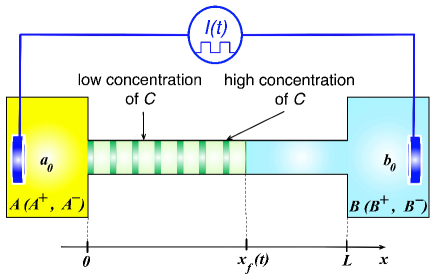
Figure 2: Experimental setup for producing Liesegang precipitation patterns as described in Sec. 2.1. The controlling agent is the generator providing electric current $I(t)$ with a prescribed time-dependence (figure is taken from [9]).

The second method keeps the time law unchanged and aims at controlling the creation time $t_{n}$ of the $n$-th band. Recalling that $t_{n}$ is the instant when the concentration of $C$-s crosses the threshold value $c^{*}$, one recognizes that $t_{n}$ can be controlled by regulating the concentration $c_{0}(x)$ at the front. Recently, it was shown both theoretically and experimentally that the above method can be made to work by sending a time-dependent electric current through the system [9]. The schematic setup for control is shown in Fig.2 and, at a phenomenological level, its working can be understood rather easily. Indeed, consider an imposed current which drives the reacting ions towards the reaction zone (we shall refer to this current as forward current). It is clear that the forward current enhances the production of $C$-s in the reaction zone. Reversing the direction of current (backward current), on the other, hand works against the reaction and results in a lower production of $C$-s. Thus, provided the position of the front is known [i.e. $x_{n}(t)$ is available from the time-law], the times $t_{n}$ of crossing of the threshold concentration and, consequently, the positions of the band $x_{n}(t_{n})$ can be controlled by an appropriately chosen current. Since managing the electric current is not an experimental difficulty, the above method provides us a flexible technique for the creation of complex precipitation patterns.

3.2 Mathematical description of the process

For a more quantitative description of the control-by-current method, we shall use a mean field model that has been developed in a series of papers during the last decade [9, 12, 23, 24]. The first part of the model addresses the irreversible $A^{+}+B^{-}\to C$ reaction-diffusion process for totally dissociated electrolytes $A\equiv(A^{+},A^{-})$ and $B\equiv(B^{+},B^{-})$ that are initially separated in space. The evolution equations for the concentration profile of the ions $a^{\pm}(x,t)$ and $b^{\pm}(x,t)$ are obtained by assuming electroneutrality on the relevant time and lengthscales [23] and, for the case of monovalent ions with equal diffusion coefficients, the equations are as follows [9]

$$\partial_{t}a^{+} = D\partial^{2}_{x}a^{+}-j(t)\,\partial_{x}(a^{+}/\Sigma)-ka^{+}b^{-}$$ (1)

$$\partial_{t}b^{-} = D\partial^{2}_{x}b^{-}+j(t)\,\partial_{x}(b^{-}/\Sigma)\,-ka^{+}b^{-}$$ (2)

$$\partial_{t}a^{-} = D\partial^{2}_{x}a^{-}+j(t)\,\partial_{x}(a^{-}/\Sigma)$$ (3)

$$\partial_{t}b^{+} = D\partial^{2}_{x}b^{+}-j(t)\,\partial_{x}(b^{+}/\Sigma)\,.$$ (4)

Here $D$ is the diffusion coefficient of the ions, $j(t)=I(t)/{\cal A}$ is the externally controlled electric current-density flowing through the tube of cross section ${\cal A}$, and $\Sigma=q(a^{+}+a^{-}+b^{+}+b^{-})$ with $q$ being the unit of charge. The reaction rate $k$ is taken to be large resulting in a reaction zone of negligible width. Note that this assumption is compatible with the typical reactions used in experimental setups producing Liesegang structures.

The second part of the model explains the pattern formation through the separation of the reaction product $C$ into a high- and low-concentration phases. The evolution of the concentration $c(x,t)$ is obtained from the Cahn-Hilliard equation with the addition of a source term corresponding to the rate of the production of $C$-s ($ka^{+}b^{-}$) [12, 24]. The free energy driving the phase separation is assumed to have minima at some low ($c_{l}$) and high ($c_{h}$) concentrations of $C$ and, furthermore, it is assumed to have the Landau-Ginzburg form in the shifted and rescaled concentration variable $m=(2c-c_{h}-c_{l})/(c_{h}-c_{l})$. In terms of $m$, the equation describing the phase-separation dynamics takes the form [12]

$$\partial_{t}m=-\lambda\Delta(m-m^{3}+\sigma\Delta m)+S(x,t)\;.$$ (5)

Here $S(x,t)=2ka^{+}b^{-}/(c_{h}-c_{l})$ is the source term coming from equations (1–4). The two parameters $\lambda$ and $\sigma$ are fitting parameter at this stage, they can be chosen so as to reproduce the correct experimental time- and lengthscales [25, 24].

Equations (1-5) are a closed set of equations for the concentrations of the electrolytes ($a^{\pm}$, $b^{\pm}$) and of the reaction product $c$. Together with the specification of the initial- and the boundary conditions, they provide the mathematical formulation of the problem. Below we shall consider numerical solutions of these equations which were obtained by the classical fourth-order Runge-Kutta method.

3.3 Simulation results - properties of the front in the presence of a current

In order to obtain a more detailed understanding of the front dynamics, we studied the numerical solution of eqs. (1) with initial conditions of separated electrolytes [$a^{\pm}(x<0,t=0)=a_{0}$, $a^{\pm}(x>0,t=0)=0$, $b^{\pm}(x<0,t=0)=0$, $b^{\pm}(x>0,t=0)=b_{0}$], and monitored both the position of the front $x_{f}(t)$ and the rate of production $S=kab$ of the $C$-s (a brief account of these simulations has appeared in [9]). The physical parameters in the equations were chosen to be close to the experimentally relevant values ($a_{0}/b_{0}=100$, $D=1.22\cdot 10^{-9}\;\mbox{m}^{2}/\mbox{s}$, $\sigma=10^{-8}\;\mbox{m}^{2}$, $\lambda=0.17\cdot 10^{-9}\;\mbox{m}^{2}/\mbox{s}$) and we considered following scenarios for the current. The no current case was used to reproduce the known front properties (i-iii). Constant forward and backward currents of amplitude $|j|=10\;\mbox{A}/\mbox{m}^{2}$ were simulated to check whether the time law holds on the experimentally relevant timescales. Finally, we studied the most interesting case of an alternating current of constant absolute value ($|j|=10\;\mbox{A}/\mbox{m}^{2}$) with the sign of it changing in a square wave pattern at times $\tau n^{2}$, with $n=0,1,2,\ldots$, and $\tau$ fixing the timescale of the protocol.

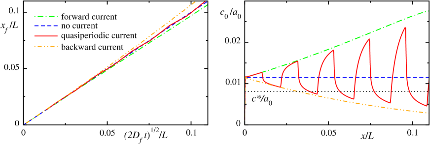
Figure 3: Left panel: The position of the reaction front (measured in units of the length $L$ of the gel column) versus diffusion length in the absence of a current, displayed for constant forward or backward current, and for a quasiperiodic current (changed at times $\tau n^{2}$). Right panel: Concentrations of the reaction product in the wake of the front for the cases considered on the left panel [9].

The results are shown on Fig.3. The left panel displays the front motion and shows that in all cases the diffusive nature of the front is hardly changed, i.e. the time law (a) remains valid. On the other hand, as can be seen on the right panel of Fig.3, the $C$-production at the front is strongly influenced by the character of the applied current. Backward current leads to a decrease of the concentration of $C$-s left behind the front, and $c_{0}(x)$ reaches values below the phase separation threshold $c_{0}(x)<c^{*}$ thus eliminating the possibility of precipitation. In contrast, the forward current increases the $C$-production steeply and brings the system quickly into the unstable regime thus inducing precipitation. It follows then that, in the case of a quasiperiodic current, the phase separation can be triggered and timed by switching on the forward field.

4 Pattern design

4.1 Controlling the spacing and the width of the bands

Once the front dynamics, summarized in Fig.3, is understood, one can invent appropriate current dynamics that results e.g. in equidistant band patterns [9]. The wavelength $d$ of the periodic pattern can be predesigned by switching on the forward currents at times $t_{n}=(2n)^{2}\tau$, where $n=0,1,2,\ldots$ and $\tau=d^{2}/8D_{f}$. If the desired period $d$ is smaller than half the local wavelength of the Liesegang pattern which would be present without the current (see Fig.1), then spurious bands may appear due to a natural increase of the concentration of $C$-s. This can be avoided, however, by switching on the backward current when the front is halfway between $x_{n}$ and $x_{n+1}$, i.e., at times $(2n+1)^{2}\tau$.

One can also create more complex patterns both experimentally and theoretically [9]. When creating patterns of several wavelengths, variable widths of the bands may also become an important part of the patterns. The issue of the width control, treated below, is the novel aspect of the present paper.

Let us begin by finding an estimate of the width of the equidistant bands having a period $d=\sqrt{8D_{f}\tau}$. From simulations we know that even in the presence of current, the position of the front is well approximated by $x_{f}(t)=\sqrt{2D_{f}t}$ where $D_{f}$ is given by [13]:

$$D_{f}=2D\left\{\mbox{erf}^{-1}\left[\frac{a_{0}/b_{0}-1}{a_{0}/b_{0}+1}\right]\right\}^{2}\;.$$ (6)

For a typical ratio of the initial concentrations of A and B, $a_{0}/b_{0}=100$, this yields $D_{f}=5.43D$, where $D$ is the diffusion constant of the ions.

An important point now is that simulations of the equidistant case [i.e. when the forward currents is switched on at times $t_{n}=(2n)^{2}\tau$] reveal (see Fig.4) that, although the $C$-production varies strongly within a period, the average concentration is practically equal to the zero current case. This means that, for the estimation of the width, we can replace the complicated function $c_{0}(x)$ by the result of the homogeneous production of $C$-s [14]:

$$c_{0}(x) \approx c_{0}=a_{0}\frac{1+b_{0}/a_{0}}{2\sqrt{\pi}}e^{-D_{f}/(2D)}\sqrt{\frac{2D}{D_{f}}}\;.$$ (7)

For $a_{0}/b_{0}=100$ this yields $c_{0}/a_{0}\approx 1.145\times 10^{-2}$.

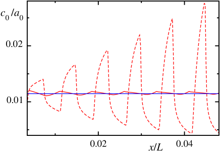
Figure 4: $C$-concentration in the wake of the front for the equidistant pattern (red dashed line) and its average over a region of distance $d$ (red solid line) in comparison with the no-current case (blue line).

Using now the conservation of $C$-s, namely that the amount of $C$-s produced in a period ($d\,c_{0}$) is distributed into the high- and low-concentration regions of length $w$ and $d-w$, the width of the bands, $w$, is calculated as

$$w = \frac{c_{0}-c_{l}}{c_{h}-c_{l}}d=\frac{c_{0}-c_{l}}{c_{h}-c_{l}}\sqrt{8D_{f}\tau}\;,$$ (8)

and we find that the width depends on $\tau$ in the same way as the period. The width also depends on the diffusion constant of the front, $D_{f}$ which, in turn, depends on the ratios of initial concentrations $a_{0}/b_{0}$ as well as on the diffusion coefficients of the electrolytes. Most easily, however, the width can tuned by the initial concentration of $A$, $a_{0}$ which is proportional to $c_{0}$.

In Fig.5 one can see the numerical verification of the above approximations for the width and the wavelength of the periodic pattern. The smaller the value of $\tau$ the better is the estimate, since for large values of $\tau$ we enter a regime where the deviations from the time-law (a) become significant.

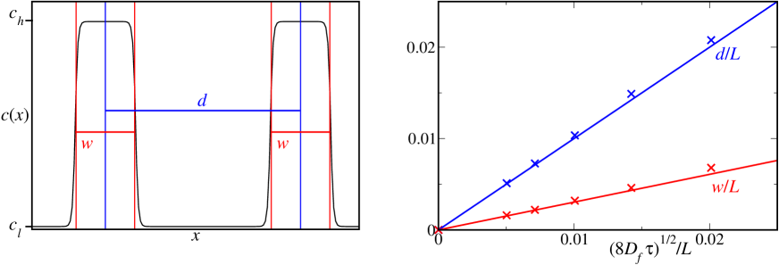
Figure 5: Left panel: Definition of the width $w$ and the period $d$ of the equidistant pattern. Right panel: Dependence of the numerically obtained widths (red cross) and periods (blue cross) on $\tau$ in comparison with the theoretical prediction (solid lines).

4.2 Encoding information into precipitation structures

Since spacing and width can be controlled by properly designed current, more complex structures should be realizable. The pattern shown in Fig. 6 has been created using a slightly generalized method of control described above for the periodic pattern. The underlying pattern in Fig. 6 is an equidistant pattern but the width of certain bands is increased. This has been achieved by a longer time interval for the forward field for the wide bands. More precisely, in order to make the width of the $n$-th band larger, the switching protocol is changed: instead of switching on the backward current at time $(2n+1)^{2}\tau$, it is switched on at time $((2n+f)^{2}\tau$ such that the band appears approximately a factor $f$ larger. Similarly it is also possible to increase the spaces between the bands by increasing the time duration of the backward current. In Fig. 7 we demonstrate this by creating a structure (the Morse code of the famous number 42 [26]) where a current dynamics had to be designed which yields simultaneous control of the spacing and the width of the bands.

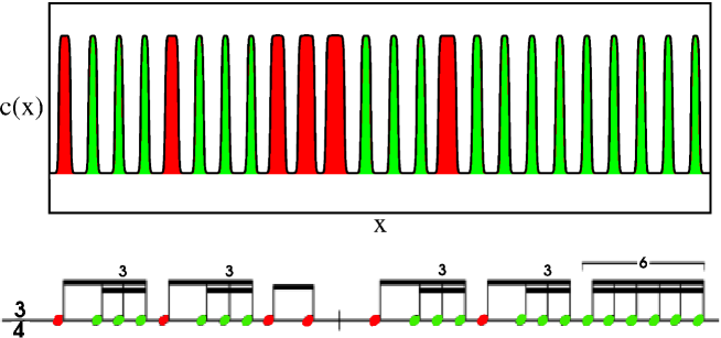
Figure 6: Musical rhythm written into Liesegang bands. The upper panel shows the concentration-profile of narrow and wide bands (the first four bands are cut out of the picture as well as the final ones since they don’t belong to the implementation of the rhythm). This is compared in the lower panel to the Bolero rhythm composed by Ravel [27] .

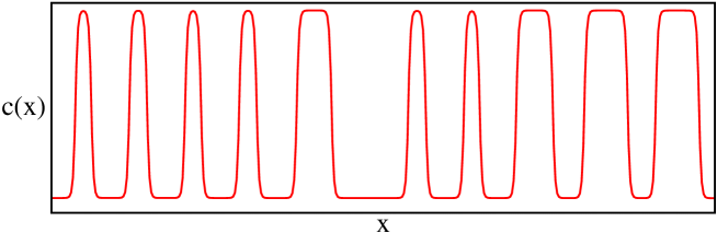
Figure 7: Concentration profile, $c(x)$ for a numerical test of the combined width and space control. In the simulation the number “42” is written into precipitation bands based on the Morse alphabet: 4 (…._) 2 (..___). The dots are implemented by narrow bands, the underscore by a wide band approximately a factor $f=2$ larger, and the characters are separated by spaces, widened by the same factor $f$.

5 Conclusions and outlook

We have developed further the techniques of the engineering of precipitation structures using electric currents. It was shown that an appropriately designed time-dependent current allows to control not only the band-spacing but also the width of the bands in one-dimensional structures. This permits the encoding of information by controlling either only the the width (as exemplified by the Bolero rhythm) or by combining the width and space control (as was shown on the example of the famous number 42).

A naturally arising question concerns the limits of the approach when trying to downscale the structures. As far as the timescales are considered, since the diffusion coefficients of the participating agents are of order $10^{-9}$ $\mbox{m}^{2}$/s, imposed currents on the time scale of $\tau=0.1s$ provide control on lengthscales of $10\mu$. Thus scaling the dynamics of the current does not pose an experimental problem.

The real problem with downscaling is the width of the bands. The minimum width is clearly related to the width of the reaction front which is not negligible on the scale of microns and, depending on the reagents, can be even at the scale of $mm$-s [28]. It should be noted however that spontaneous pattern formation on the nanoscale level has been observed [29], and these type of systems might be appropriate for the pattern control by imposed electric currents. Another problem with the width of the bands is that the thermal fluctuations in the concentrations of the reagents combined with those of the gel make the reaction front uneven and, depending on the surface tension of the created bands, they may lead to a roughening of the band on a scale that is comparable to the width. Clearly, advances in downscaling can be achieved only if models are developed which can treat all the above problems.

Finally, we note that combining the proposed technique with the already existing indirect control strategies such as the choice of geometry and initial conditions opens up a wide spectrum of possible structure design. So far the feasibility of the approach has only been shown for a few types of predesigned one-dimensional patterns. A straightforward extention would be the creation of rings or spheres with a predesigned internal structure. Further, the extention of the current-control technique to stamping methods [5] on the mesoscopic level could be used to create even more complex pattern designs which may become useful in engineering applications.

References

References

- [1] Shinbrot T and Muzzio F J, Noise to order, 2001 Nature 410 251-258
- [2] For a review see Cross M C and Hohenberg P C, Pattern formation outside of equilibrium, 1994 Rev. Mod. Phys. 65 851-1112
- [3] Henisch H K, Periodic precipitation, 1991 Pergamon Press, New York
- [4] Lu W and Lieber C M, Nanoelectronics from the bottom up, 2007 Nat. Mater. 6 841-850
- [5] Bensemann I T, Fialkowski M and Grzybowski B A, Wet Stamping of Microscale Periodic Precipitation Patterns, 2005 J. Phys. Chem. B 109 2774
- [6] Giraldo O, Brock S L, Marquez M, Suib S L, Hillhouse H and Tsapatsis M, Spontaneous formation of inorganic helices, 2000 Nature 405 38-38-2778
- [7] Lebedeva M I, Vlachos D G and Tsapatsis M, Bifurcation Analysis of Liesegang Ring Pattern Formation, 2004 Phys. Rev. Lett. 92 088301-1-4
- [8] Antal T, Bena I, Droz M, Martens K and Rácz Z, Guiding fields for phase separation: Controlling Liesegang patterns, 2007 Phys. Rev. E 76 046203-1-9
- [9] Bena I, Droz M, Lagzi I, Martens K, Rácz Z and Volford A, Designer Patterns: Flexible Control of Precipitation through Electric Currents, 2008 Phys. Rev. Lett. 101 075701
- [10] Liesegang R E, Ueber einige Eigenschaften von Gallerten, 1896 Naturwiss. Wochenschr. 11 353-362
- [11] Dee G T, Patterns produced by precipitation at a moving reaction front,1986 Phys. Rev. Lett. 57 275-278
- [12] Antal T, Droz M, Magnin J and Rácz Z, Formation of Liesegang patterns: A spinodal decomposition scenario, 1999 Phys. Rev. Lett. 83 2880-2883
- [13] Gálfi L and Rácz Z, Properties of the reaction front in an type reaction-diffusion process, 1988 Phys. Rev. A 38 3151-3154
- [14] Antal T, Droz M, Magnin J, Rácz Z and Zrinyi M, Derivation of the Matalon-Packter law for Liesegang patterns, 1998 J. Chem. Phys. 109 9479-9486
- [15] Morse H W and Pierce G W, Diffusion and Supersaturation in Gelatine, 1903 PAAAS 38 625-647
- [16] Jablczynski K, La formation rythmique des précipités: Les anneaux de Liesegang, 1923 Bull. Soc. Chim. France 33 1592-1603
- [17] Müller S C, Kai S and Ross J, Periodic precipitation patterns in the presence of concentration gradients. 1. Dependence on ion product and concentration difference, 1982 J. Phys. Chem. 86 4078-4087
- [18] Cahn J W and Hilliard J E, Free Energy of a Nonuniform System. I. Interfacial Free Energy, J. Chem. Phys. 1958 28, 258-267; Cahn J W, On spinodal decomposition, 1961 Acta Metall. 9 795-801
- [19] Matalon R and Packter A, The Liesegang phenomenon I. Sol protection and diffusion, 1955 J. Colloid Sci. 10 46-62; A. Packter, The Liesegang phenomenon. IV: Reprecitation from ammoniapeptized sols, 1955 Kolloid Z. 142 109-117
- [20] Bena I, Droz M, Martens K and Rácz Z, Reaction-diffusion fronts with inhomogeneous initial conditions, 2007 J. Phys.: Condens. Matter 19 065103
- [21] Yuste S B, Acedo L and Lindenberg K, Reaction front in an reaction-subdiffusion process, 2004 Phys. Rev. E 69 036126
- [22] Rongy L, Trevelyan P M J and De Wit A, Dynamics of Reaction Fronts in the Presence of Bouyancy-Driven Convection, 2008 Phys. Rev. Lett. 101 084503
- [23] Bena I, Coppex F, Droz M and Rácz Z, Front motion in an type reaction-diffusion process: Effects of an electric field, 2005 J. Chem. Phys. 122 024512-1-11
- [24] Bena I, Droz M and Rácz Z, Formation of Liesegang patterns in the presence of an electric field, 2005 J. Chem. Phys. 122 204502-1-9
- [25] Rácz Z, Formation of Liesegang Patterns, 1999 Physica A 274 50-59
- [26] Adams D, The Hitchhiker’s Guide to the Galaxy, 2002 Ballantine Books, New York
- [27] The wide bands emerging at later stages are wider because because we enter a regime where the approximation of the homogeneous production of ’s is no longer valid due to the long duration of the forward fields (see Fig. 1).
- [28] Koo Y-E L and Kopelman R, Space- and time-resolved diffusion-limited binary reaction kinetics in capillaries: Experimental observation of segregation, anomalous exponents, and depletion zone, 1991 J. Stat. Phys. 65 893
- [29] Mohr C, Dubiel M and Hofmeister H, Formation of silver particles and periodic precipitate layers in silicate glass induced by thermally assisted hydrogen permeation, 2001 J. Phys. Condensed Matter 13 525