Entanglement Dynamics in Two-Qubit Open System Interacting with a Squeezed Thermal Bath via Quantum Nondemolition interaction

Abstract

We analyze the dynamics of entanglement in a two-qubit system interacting with an initially squeezed thermal environment via a quantum nondemolition system-reservoir interaction, with the system and reservoir assumed to be initially separable. We compare and contrast the decoherence of the two-qubit system in the case where the qubits are mutually close-by (‘collective regime’) or distant (‘localized regime’) with respect to the spatial variation of the environment. Sudden death of entanglement (as quantified by concurrence) is shown to occur in the localized case rather than in the collective case, where entanglement tends to ‘ring down’. A consequence of the QND character of the interaction is that the time-evolved fidelity of a Bell state never falls below $1/\sqrt{2}$, a fact that is useful for quantum communication applications like a quantum repeater. Using a novel quantification of mixed state entanglement, we show that there are noise regimes where even though entanglement vanishes, the state is still available for applications like NMR quantum computation, because of the presence of a pseudo-pure component.

I Introduction

Open quantum systems are ubiquitous in the sense that any system can be thought of as being surrounded by its environment (reservoir or bath) which influences its dynamics. They provide a natural route for discussing damping and dephasing. One of the first testing grounds for open system ideas was in quantum optics wl73 . Its application to other areas gained momentum from the works of Caldeira and Leggett cl83 , and Zurek wz93 , among others. The total Hamiltonian is $H=H_{S}+H_{R}+H_{SR}$ , where $S$ stands for the system, $R$ for the reservoir and $SR$ for the system-reservoir interaction. The evolution of the system of interest $S$ is studied taking into account the effect of its environment $R$, through the $SR$ interaction term, making the resulting dynamics non-unitary. Depending upon the system-reservoir ($S-R$) interaction, open systems can be broadly classified into two categories, viz., quantum non-demolition (QND), which we consider here, or dissipative (cf. for example Ref. ingold ). A particular type of quantum nondemolition (QND) $S-R$ interaction is given by a class of energy-preserving measurements in which dephasing occurs without damping the system, i.e., where $[H_{S},H_{SR}]=0$ while the dissipative systems correspond to the case where $[H_{S},H_{SR}]\neq 0$ resulting in decoherence along with dissipation bg07 .

A class of observables that may be measured repeatedly with arbitrary precision, with the influence of the measurement apparatus on the system being confined strictly to the conjugate observables, is called QND or back-action evasive observables bvt80 ; bk92 ; wm94 ; zu84 . Such a measurement scheme was originally introduced in the context of the detection of gravitational waves ct80 ; bo96 . The energy preserving measurements, referred to above, form an important class of such a general QND measurement scheme.

The interest in the relevance of open system ideas to quantum information has increased in recent times because of the impressive progress made, and the potential for future progress (cf. for example Ref. erika ), on the experimental front in the manipulation of quantum states of matter towards quantum information processing and quantum communication. Myatt et al. myatt and Turchette et al. turch have performed a series of experiments in which they induced decoherence and decay by coupling the atom (their system-$S$) to engineered reservoirs, in which the coupling to, and the state of, the environment are controllable. An experiment reported in Ref. jb03 demonstrated and completely characterized a QND scheme for making a nondeterministic measurement of a single photon nondestructively using only linear optics and photo-detection of ancillary modes, to induce a strong nonlinearity at the single photon level. The dynamics of decoherence in continuous atom-optical QND measurements has been studied in vo98 .

Quantum entanglement is the inherent property of a system to exhibit correlations, the physical basis being the non-local nature of quantum mechanics bell , and hence is a property that is exclusively quantum in nature. Entanglement plays a central role in quantum information theory nc , in quantum computation as in the Shor algorithm shor , and quantum error correction css . A number of methods have been proposed for creating entanglement involving trapped atoms beige ; fy00 ; sm02 .

An important issue is to study how quantum entanglement is affected by noise, which can be thought of as a manifestation of an open system effect bp02 . A recent experimental investigation of the dynamics of entanglement with a continuous monitoring of the environment, i.e., via a realization of quantum trajectories car93 , has been made in am07 . Here we study the effect of noise on the entanglement generated between two spatially separated qubits, by means of their interaction with the bath, which is taken to be in an initial squeezed-thermal state bg07 ; sqgen . This is of relevance to evaluate the performance of two-qubit gates in practical quantum information processing systems. The two qubits are intially uncorrelated. With the advent of time entanglement builds up between them via their interaction with the bath but eventually gets destroyed because of the quantum to classical transition mediated by the noise. In this paper we study the effect of noise generated by a QND $S-R$ interaction. The issue of a dissipative noise is taken up in a separate work.

Since we are dealing here with a two qubit system which very rapidly evolves into a mixed state, a study of entanglement would necessarily involve a measure of entanglement for mixed states. Entanglement of a bipartite system bz08 in a pure state is unambigious and well defined. However, mixed state entanglement (MSE) is not so well defined. Thus, although a number of criteria such as entanglement of formation bd96 ; ww98 ; mc05 and negativity fw89 exist, there is a realization bd96 that a single quantity is inadequate to describe MSE. This was the principal motivation for the development of a new prescription of MSE br08 in which it is characterized not by a number, but as a probability density function (PDF). This generalization provides an exhaustive and geometrical characterization of entanglement : by exploring the entanglement content in the various subspaces spanning the two-qubit Hilbert space. The known prescriptions such as concurrence and negativity emerge as particular elements in the set of parameters that characterize the probability density function. We will study entanglement in the two-qubit system using concurrence as well as the probability density function.

The plan of the paper is as follows. In Sections II and III, we develop our open system model for the multi-qubit dynamics under the influence of a QND $S-R$ interaction. Section II develops the general dynamics for a multi-qubit system, where the qubits are spatially separated and initially uncorrelated, and the bath is in a general squeezed-thermal state. Section III specializes these considerations to the case of two qubits. In Section IV, we point out some interesting symmetries obeyed by the two-qubit dynamics. Section V makes a brief application of the model to practical quantum communication, in particular, in the realization of a quantum repeater chb96 ; bdcz98 . In Section VI, we give a brief description of the recently developed entanglement measure of MSE br08 . Section VII deals with the entanglement analysis of the two-qubit open system using the PDF as a measure of entanglement. We also dwell upon the usual measure of MSE, concurrence. We deal with the scenarios where the two qubits effectively interact via localized $S-R$ interactions, called the localized (independent) decoherence model, as also when they interact collectively with the bath, called the collective decoherence model. The usefulness of the PDF measure of entanglement is that it allows us to demonstrate the existence of noise regimes where even though entanglement vanishes, the state is still available for applications like NMR quantum computation, because of the presence of a pseudo-pure component. In Section VIII, as an application of the PDF, we make a brief discussion of the temperature dependent effective dynamics obeyed by the two-qubit open system in the collective decoherence regime. In Section IX, we make our conclusions.

II Multi -Qubit QND interaction with a Squeezed Thermal Bath

We consider the Hamiltonian, describing the QND interaction of $L$ qubits with the bath as rj02 ; bg07 ; bgg07

$$H = H_{S}+H_{R}+H_{SR}$$ (1)

$$= \sum\limits_{n=1}^{L}\hbar\varepsilon_{n}J^{n}_{z}+\sum\limits_{k}\hbar\omega_{k}b^{\dagger}_{k}b_{k}+\sum\limits_{n,k}\hbar J^{n}_{z}(g^{n}_{k}b^{\dagger}_{k}+g^{n*}_{k}b_{k}).$$

Here $H_{S}$, $H_{R}$ and $H_{SR}$ stand for the Hamiltonians of the system, reservoir and system-reservoir interaction, respectively. $b^{\dagger}_{k}$, $b_{k}$ denote the creation and annihilation operators for the reservoir oscillator of frequency $\omega_{k}$, $g^{n}_{k}$ stands for the coupling constant (assumed to be position dependent) for the interaction of the oscillator field with the qubit system and are taken to be

$$g^{n}_{k}=g_{k}e^{-ik.r_{n}},$$ (2)

where $r_{n}$ is the qubit position. Since $[H_{S},H_{SR}]=0$, the Hamiltonian (1) is of QND type. In the parlance of quantum information theory, the noise generated is called the phase damping noise gp06 ; bg07 .

The position dependence of the coupling of the qubits to the bath (2) helps to bring out the effect of entanglement between qubits through the qubit separation: $r_{mn}\equiv r_{m}-r_{n}$. This allows for a discussion of the dynamics in two regimes: (A). localized decoherence where $k.r_{mn}\sim\frac{r_{mn}}{\lambda}\geq 1$ and (B). collective decoherence where $k.r_{mn}\sim\frac{r_{mn}}{\lambda}\rightarrow 0$. The case (B) of collective decoherence would arise when the qubits are close enough for them to experience the same environment, or when the bath has a long correlation length (set by the effective wavelength $\lambda$) compared to the interqubit separation $r_{mn}$ rj02 . Our aim is to study the reduced dynamics of the qubit system. As in the case of a single qubit QND interaction with bath bg07 ; bgg07 , the density matrix is evaluated in the system eigenbasis $|i_{n}\rangle=|\pm\frac{1}{2}\rangle$ (the possible eigenstates of $J^{n}_{z}$ with eigenvalues $j_{n}=\pm\frac{1}{2}$). The system-plus-reservoir composite is closed and hence obeys a unitary evolution given, in the interaction picture, by

$$\rho(t)=U_{I}(t)\rho(0)U^{\dagger}_{I}(t),$$ (3)

where

$$U_{I}(t)={\cal T}e^{-(i/\hbar)\int_{0}^{t}dt^{\prime}H_{I}(t^{\prime})},$$ (4)

with $H_{I}(t)=e^{i(H_{S}+H_{R})t/\hbar}H_{SR}e^{-i(H_{S}+H_{R})t/\hbar}$, and ${\cal T}$ denotes time ordering. Also

$$\rho(0)=\rho^{s}(0)\rho_{R}(0),$$ (5)

i.e., we assume separable initial conditions. Here

$$\rho^{s}(0)=\rho^{s}_{1}(0)\otimes\rho^{s}_{2}(0)\cdots\otimes\rho^{s}_{L}(0),$$ (6)

is the initial state of the qubit system and the subscripts denote the individual qubits. In Eq. (5), $\rho_{R}(0)$ is the initial density matrix of the reservoir which we take to be a broadband squeezed thermal bath bg07 ; bgg07 ; gp06 given by

$$\rho_{R}(0)=S(\alpha,\Phi)\rho_{th}S^{\dagger}(\alpha,\Phi),$$ (7)

where

$$\rho_{th}=\prod_{k}\left[1-e^{-\beta\hbar\omega_{k}}\right]e^{-\beta\hbar\omega_{k}b^{\dagger}_{k}b_{k}}$$ (8)

is the density matrix of the thermal bath at temperature $T$, with $\beta\equiv 1/(k_{B}T)$, $k_{B}$ being the Boltzmann constant, and

$$S(\alpha_{k},\Phi_{k})=\exp\left[\alpha_{k}\left({b^{2}_{k}\over 2}e^{-2i\Phi_{k}}-{b^{\dagger 2}_{k}\over 2}e^{2i\Phi_{k}}\right)\right]$$ (9)

is the squeezing operator with $\alpha_{k}$, $\Phi_{k}$ being the squeezing parameters cs85 .

In order to obtain the reduced dynamics of the system , we trace over the reservoir variables. The matrix elements of the reduced density matrix in the system eigenbasis are obtained for the localized and collective decoherence models as:

II.1 Localized decoherence model

$$\rho^{s}_{\{i_{n},j_{n}\}}(t)=\exp[i\{\Theta_{\{i_{n},j_{n}\}}^{\rm{lc}}(t)-\Lambda_{\{i_{n},j_{n}\}}^{\rm{lc}}(t)\}]\exp[-\Gamma^{\rm{lc}}_{\{i_{n},j_{n}\}(\rm{sq})}(t)]\rho^{s}_{\{i_{n},j_{n}\}}(0).$$ (10)

Here $\rho^{s}_{\{i_{n},j_{n}\}}(t)$ stands for $\langle i_{L},i_{L-1},...,i_{1}|{\rm Tr}_{R}{\rho^{s}(t)}|j_{L},j_{L-1},...,j_{1}\rangle$ and the symbol ${\{i_{n},j_{n}\}}$ stands collectively for ${i_{1},j_{1};i_{2},j_{2};...;i_{L},j_{L}}$. The superscript lc is to indicate that these expressions are for the localized decoherence model and the subscript sq indicates that the bath starts in a squeezed thermal initial state. As seen from the expressions given below, $\Theta_{\{i_{n},j_{n}\}}^{\rm{lc}}$ and $\Lambda_{\{i_{n},j_{n}\}}^{\rm{lc}}$ are independent of the bath initial conditions and are given in the continuum limit (assuming a quasi-continuous bath spectrum) by

$$\Theta_{\{i_{n},j_{n}\}}^{\rm{lc}}(t)=2\int\limits^{\infty}_{0}d\omega I(\omega)S(\omega,t)\sum^{L}_{\stackrel{{\scriptstyle m=1,n=2}}{{(m\neq n)}}}(i_{m}i_{n}-j_{m}j_{n})\cos(\omega t_{s}),$$ (11)

$$\Lambda_{\{i_{n},j_{n}\}}^{\rm{lc}}(t)=2\int\limits^{\infty}_{0}d\omega I(\omega)C(\omega,t)\sum^{L}_{(m\neq n)}i_{m}j_{n}\sin(\omega t_{s}).$$ (12)

In the above equations, $I(\omega)$ is the bath spectral density given in terms of the system (qubits) and bath coupling constant as $I(\omega)=\sum\limits_{k}\delta(\omega-\omega_{k})g^{2}_{k}$, which for the Ohmic case considered here has the form

$$I(\omega)={\gamma_{0}\over\pi}\omega e^{-\omega/\omega_{c}},$$ (13)

where $\gamma_{0}$ and $\omega_{c}$ are two bath parameters. Also

$$S(\omega,t)=\frac{\omega t-\sin(\omega t)}{\omega^{2}},$$ (14)

and

$$C(\omega,t)=\frac{1-\cos(\omega t)}{\omega^{2}}.$$ (15)

In Eqs. (11) and (12), $\omega t_{s}\equiv k.r_{mn}$ rj02 , where $t_{s}$ is the transit time introduced in order to express the system-bath coupling in the frequency domain. $\Gamma^{lc}_{sq}(t)$ in Eq. (10) is given as

$$\Gamma^{\rm{lc}}_{\{i_{n},j_{n}\}(\rm{sq})}(t) = \int\limits^{\infty}_{0}d\omega I(\omega)\coth(\frac{\beta\hbar\omega}{2})$$ (16)

$$\times \left[\cosh(2\alpha)C(\omega,t)\Big{\{}\sum^{L}_{m=1}(i_{m}-j_{m})^{2}+2\sum^{L}_{\stackrel{{\scriptstyle m=1,n=2}}{{(m\neq n)}}}(i_{m}-j_{m})(i_{n}-j_{n})\cos(\omega t_{s})\Big{\}}\right.$$

$$- \left.\frac{2}{\omega^{2}}\sin^{2}(\frac{\omega t}{2})\sinh(2\alpha)\Big{\{}\cos(\omega(t-2a))[\sum^{L}_{m=1}(i_{m}-j_{m})^{2}\cos(\omega t_{corr1})\right.$$

$$+ \left.2\sum^{L}_{\stackrel{{\scriptstyle m=1,n=2}}{{(m\neq n)}}}(i_{m}-j_{m})(i_{n}-j_{n})\cos(\omega t_{corr2})]+\sin(\omega(t-2a))[\sum^{L}_{m=1}(i_{m}-j_{m})^{2}\sin(\omega t_{corr1})\right.$$

$$+ \left.2\sum^{L}_{\stackrel{{\scriptstyle m=1,n=2}}{{(m\neq n)}}}(i_{m}-j_{m})(i_{n}-j_{n})\sin(\omega t_{corr2})]\Big{\}}\right],$$

where we have defined two new time scales $\omega t_{corr1}\equiv 2k.r_{m}$ and $\omega t_{corr2}\equiv k.(r_{n}+r_{m})$ which are due to the non-stationary effects introduced by the squeezed thermal bath. Here we have for simplicity taken the squeezed bath parameters as

$$\cosh\left(2\alpha(\omega)\right) = \cosh(2\alpha),~{}~{}\sinh\left(2\alpha(\omega)\right)=\sinh(2\alpha),$$

$$\Phi(\omega) = a\omega,$$ (17)

where $a$ is a constant depending upon the squeezed bath.

II.2 Collective decoherence model

The reduced density matrix is given by

$$\rho^{s}_{\{i_{n},j_{n}\}}(t)=\exp[i\{\Theta_{\{i_{n},j_{n}\}}^{\rm{col}}(t)-\Lambda_{\{i_{n},j_{n}\}}^{\rm{col}}(t)\}]\exp[-\Gamma^{\rm{col}}_{\{i_{n},j_{n}\}(\rm{sq})}(t)]\rho^{s}_{\{i_{n},j_{n}\}}(0).$$ (18)

The superscript $\rm{col}$ is to indicate that these expressions are for the collective decoherence model and the subscript $\rm{sq}$ indicates that the bath starts in a squeezed thermal initial state. As in the case of localized decoherence, $\Theta^{\rm{col}}$ and $\Lambda^{\rm{col}}$ are independent of the bath initial conditions and are given in the continuum limit (assuming a quasi-continuous bath spectrum) by

$$\Theta^{\rm{col}}(t)=\int\limits^{\infty}_{0}d\omega I(\omega)S(\omega,t)\left[(\sum^{L}_{m=1}i_{m})^{2}-(\sum^{L}_{m=1}j_{m})^{2}\right],$$ (19)

$$\Lambda^{\rm{col}}(t)=0.$$ (20)

The bath spectral density $I(\omega)$ is as in Eq. (13). In Eq. (18), $\Gamma^{\rm{col}}_{\{i_{n},j_{n}\}(\rm{sq})}(t)$ is

$$\Gamma^{\rm{col}}_{\{i_{n},j_{n}\}(\rm{sq})}(t) = \int\limits^{\infty}_{0}d\omega I(\omega)\coth(\frac{\beta\hbar\omega}{2})\left[\cosh(2\alpha)C(\omega,t)[\sum^{L}_{m=1}(i_{m}-j_{m})]^{2}\right.$$ (21)

$$- \left.\frac{2}{\omega^{2}}\sin^{2}(\frac{\omega t}{2})\sinh(2\alpha)\Big{\{}\cos(\omega(t-2a))[\sum^{L}_{m=1}(i_{m}-j_{m})^{2}\cos(\omega t_{corr1})\right.$$

$$+ \left.2\sum^{L}_{\stackrel{{\scriptstyle m=1,n=2}}{{(m\neq n)}}}(i_{m}-j_{m})(i_{n}-j_{n})\cos(\omega t_{corr2})]+\sin(\omega(t-2a))[\sum^{L}_{m=1}(i_{m}-j_{m})^{2}\sin(\omega t_{corr1})\right.$$

$$+ \left.2\sum^{L}_{\stackrel{{\scriptstyle m=1,n=2}}{{(m\neq n)}}}(i_{m}-j_{m})(i_{n}-j_{n})\sin(\omega t_{corr2})]\Big{\}}\right],$$

All the other terms are as defined above. On comparing Eq. (21) with (16), we find that the terms proportional to $\sinh(2\alpha)$, arising from the non-stationarity of the squeezed bath, are same while the terms proportional to $\cosh(2\alpha)$ differ from each other. For the collective decoherence model, $\omega t_{s}\equiv k.r_{mn}\equiv 0$, but the two time-scales coming from the non-stationary components of the squeezed thermal bath, i.e., $\omega t_{corr1}\equiv 2k.r_{m}$ and $\omega t_{corr2}\equiv k.(r_{n}+r_{m})$ are both non-zero, indicative of correlations induced between the qubits by the bath squeezing. For the case of zero bath squeezing, both the Eqs. (21) and (16) reduce to their corresponding values for the case of a thermal bath rj02 .

III Two qubit interaction

Here we specialize the general considerations of the previous section to the case of two qubits.

III.1 Localized decoherence model

The reduced density matrix is a specialization of Eq. (10) to the case of two qubits, say a and b. Here $\rho^{s}_{\{i_{n},j_{n}\}}(t)$ would be $\rho^{s}_{\{i_{a},j_{b}\}}(t)$ which represents $\langle i_{a},i_{b}|{\rm Tr}_{R}{\rho^{s}(t)}|j_{a},j_{b}\rangle$, where the states $|i_{a}\rangle$ or $|i_{b}\rangle$ have eigenvalues $\pm\frac{1}{2}$. We will collectively represent the two-particle index $ab$ by a single 4-level index according to the following scheme:

$$-\frac{1}{2},-\frac{1}{2}\equiv 0,~{}~{}-\frac{1}{2},\frac{1}{2}\equiv 1,~{}~{}\frac{1}{2},-\frac{1}{2}\equiv 2,~{}~{}\frac{1}{2},\frac{1}{2}\equiv 3.$$

Thus there will be sixteen elements of the density matrix, which we enumerate below. They are seen to satisfy the symmetries

$$\rho^{s}_{32}(t)=\rho^{\ast s}_{23}(t)=\rho^{s}_{01}(t)=\rho^{\ast s}_{10}(t),$$ (22)

where $\ast$ in the superscript indicates complex conjugation, and of course the first and last equality follow from the hermiticity of the density operator. In the Eqs. (22), $\Theta_{\{i_{n},j_{n}\}}^{\rm{lc}}(t)$, $\Lambda_{\{i_{n},j_{n}\}}^{\rm{lc}}(t)$ can be obtained from the Eqs. (11), (12), respectively, and $\Gamma^{\rm{lc}}_{\{i_{n},j_{n}\}(\rm{sq})}(t)$ from Eq. (16) and are given by

$$\Theta^{\rm{lc}}_{32}(t)=\Theta^{\rm{lc}}_{01}(t)=\int\limits^{\infty}_{0}d\omega I(\omega)S(\omega,t)\cos(\omega t_{s}),$$ (23)

$$\Lambda^{\rm{lc}}_{32}(t)=\Lambda^{\rm{lc}}_{01}(t)=-\int\limits^{\infty}_{0}d\omega I(\omega)C(\omega,t)\sin(\omega t_{s}),$$ (24)

$$\Theta^{\rm{lc}}_{23}(t)=\Theta^{\rm{lc}}_{10}(t)=-\Theta^{\rm{lc}}_{32}(t)=-\Theta^{\rm{lc}}_{01}(t),$$ (25)

$$\Lambda^{\rm{lc}}_{23}(t)=\Lambda^{\rm{lc}}_{10}(t)=-\Lambda^{\rm{lc}}_{32}(t)=-\Lambda^{\rm{lc}}_{01}(t),$$ (26)

and

$$\Gamma^{\rm{lc}}_{\rm{sq}}(t) = \int\limits^{\infty}_{0}d\omega I(\omega)\coth(\frac{\beta\hbar\omega}{2})\left[\cosh(2\alpha)C(\omega,t)-\frac{2}{\omega^{2}}\sin^{2}(\frac{\omega t}{2})\sinh(2\alpha)\Big{\{}\cos(\omega(t-2a))\cos(\omega t_{corr1}^{(1)})\right.$$ (27)

$$+ \left.\sin(\omega(t-2a))\sin(\omega t_{corr1}^{(1)})\Big{\}}\right],$$

for all the above combinations. In the above equations, $\omega t_{s}$ stands for $k\cdot r_{ab}$ while $\omega t_{corr1}^{(1)}\equiv 2k\cdot r_{b}$. Interestingly, for the above cases, the correlation time $\omega t_{corr2}\equiv k.(r_{a}+r_{b})$ is absent. It can be seen that

$$\rho^{s}_{aa}(t) = \rho^{s}_{aa}(0),~{}~{}~{}~{}(a=0,1,2,3),$$ (28)

from which follows that the population remains unchanged. This is a consequence of QND nature of the $S-R$ interaction. Also,

$$\rho^{s}_{21}(t)=\rho^{\ast s}_{12}(t)=\rho^{s}_{12}(t),$$

$$\rho^{s}_{30}(t)=\rho^{\ast s}_{03}(t)=\rho^{s}_{03}(t),$$ (29)

i.e., these components are purely real. In Eqs. (29), $\Theta^{\rm{lc}}(t)$, $\Lambda^{\rm{lc}}(t)$ and $\Gamma^{\rm{lc}}_{\rm{sq}}(t)$ are given by

$$\Theta^{\rm{lc}}(t)=0=\Lambda^{\rm{lc}}(t),$$ (30)

and

$$\Gamma^{\rm{lc}}_{{\rm sq},30}(t) = \Gamma^{\rm{lc}}_{{\rm sq},03}(t)=$$ (31)

$$= \int\limits^{\infty}_{0}d\omega I(\omega)\coth(\frac{\beta\hbar\omega}{2})\left[2\cosh(2\alpha)C(\omega,t)[1+\cos(\omega t_{s})]-\frac{2}{\omega^{2}}\sin^{2}(\frac{\omega t}{2})\sinh(2\alpha)\right.$$

$$\times \left.\Big{\{}\cos(\omega(t-2a))[\cos(2k\cdot r_{a})+\cos(2k\cdot r_{b})+2\cos(k\cdot[r_{a}+r_{b}])]\right.$$

$$+ \left.\sin(\omega(t-2a))[\sin(2k\cdot r_{a})+\sin(2k\cdot r_{b})+2\sin(k\cdot[r_{a}+r_{b}])]\Big{\}}\right],$$

$$\Gamma^{\rm{lc}}_{\rm{sq},21}(t) = \Gamma^{\rm{lc}}_{\rm{sq},12}(t)$$ (32)

$$= \int\limits^{\infty}_{0}d\omega I(\omega)\coth(\frac{\beta\hbar\omega}{2})\left[2\cosh(2\alpha)C(\omega,t)[1-\cos(\omega t_{s})]-\frac{2}{\omega^{2}}\sin^{2}(\frac{\omega t}{2})\sinh(2\alpha)\right.$$

$$\times \left.\Big{\{}\cos(\omega(t-2a))[\cos(2k\cdot r_{a})+\cos(2k\cdot r_{b})-2\cos(k\cdot[r_{a}+r_{b}])]\right.$$

$$+ \left.\sin(\omega(t-2a))[\sin(2k\cdot r_{a})+\sin(2k\cdot r_{b})-2\sin(k\cdot[r_{a}+r_{b}])]\Big{\}}\right].$$

Thus we see that the Eqs. (31), (32), depend on both $2k\cdot r_{a}$ and $2k\cdot r_{b}$, and $\omega t_{corr2}$ which is as defined above. Further,

$$\rho^{s}_{31}(t)=\rho^{\ast s}_{13}(t)=\rho^{s}_{02}(t)=\rho^{\ast s}_{20}(t),$$ (33)

where $\ast$ in the superscript indicates complex conjugation. In Eqs. (33), $\Theta^{\rm{lc}}(t)$, $\Lambda^{\rm{lc}}(t)$ are

$$\Theta^{\rm{lc}}_{31}(t)=\Theta^{\rm{lc}}_{02}(t)=\int\limits^{\infty}_{0}d\omega I(\omega)S(\omega,t)\cos(\omega t_{s}),$$ (34)

$$\Lambda^{\rm{lc}}_{31}(t)=\Lambda^{\rm{lc}}_{02}(t)=\int\limits^{\infty}_{0}d\omega I(\omega)C(\omega,t)\sin(\omega t_{s}),$$ (35)

$$\Theta^{\rm{lc}}_{13}(t)=\Theta^{\rm{lc}}_{20}(t)=-\Theta^{\rm{lc}}_{31}(t)=-\Theta^{\rm{lc}}_{02}(t),$$ (36)

$$\Lambda^{\rm{lc}}_{13}(t)=\Lambda^{\rm{lc}}_{20}(t)=-\Lambda^{\rm{lc}}_{31}(t)=-\Lambda^{\rm{lc}}_{02}(t),$$ (37)

and

$$\Gamma^{\rm{lc}}_{\rm{sq}}(t) = \int\limits^{\infty}_{0}d\omega I(\omega)\coth(\frac{\beta\hbar\omega}{2})\left[\cosh(2\alpha)C(\omega,t)-\frac{2}{\omega^{2}}\sin^{2}(\frac{\omega t}{2})\sinh(2\alpha)\Big{\{}\cos(\omega(t-2a))\cos(\omega t_{corr1}^{(2)})\right.$$ (38)

$$+ \left.\sin(\omega(t-2a))\sin(\omega t_{corr1}^{(2)})\Big{\}}\right],$$

for all the above combinations. In the above equations, $\omega t_{s}$ stands for $k\cdot r_{ab}$ while $\omega t_{corr1}^{(2)}\equiv 2k\cdot r_{a}$. Interestingly, for the above cases, the correlation time $\omega t_{corr2}\equiv k.(r_{a}+r_{b})$ is absent. The Eqs. (22), (28), (29) and (33) cover all the density matrices for the two-qubit localized decoherence model. It can be shown from these results that with the increase in temperature, as also evolution time $t$ and bath squeezing $\alpha$, the system becomes more mixed and hence looses its purity.

III.2 Collective decoherence model

The reduced density matrix is a specialization of Eq. (18) to the case of two qubits, say a and b. The notations are as before.

$$\rho^{s}_{32}(t)=\rho^{\ast s}_{23}(t)=\rho^{s}_{01}(t)=\rho^{\ast s}_{10}(t),$$ (39)

where $\ast$ in the superscript indicates complex conjugation. In the Eqs. (39), $\Theta^{\rm{col}}(t)$, $\Lambda^{\rm{col}}(t)$ ($=0$) are obtained from the Eqs. (19), (20), respectively and $\Gamma^{\rm{col}}_{\rm{sq}}(t)$ from Eq. (21). They are given by

$$\Theta^{\rm{in}}_{32}(t)=\Theta^{\rm in}_{01}(t)=\int\limits^{\infty}_{0}d\omega I(\omega)S(\omega,t),$$ (40)

$$\Theta^{\rm{col}}_{23}(t)=\Theta^{\rm{col}}_{10}(t)=-\Theta^{\rm{col}}_{32}(t)=-\Theta^{\rm{col}}_{01}(t),$$ (41)

and $\Gamma^{\rm{col}}_{\rm{sq}}(t)$ is as in Eq. (27) for all the cases in Eq. (39), with $\omega t_{corr1}$ and $\omega t_{corr2}$ as defined there. As before,

$$\rho^{s}_{aa}(t) = \rho^{s}_{aa}(0),~{}~{}~{}~{}(a=0,1,2,3).$$ (42)

This is indicative of QND nature of the $S-R$ interaction which preserves the population. Also,

$$\rho^{s}_{21}(t)=\rho^{\ast s}_{12}(t)=\rho^{s}_{12}(t),$$

$$\rho^{s}_{30}(t)=\rho^{\ast s}_{03}(t)=\rho^{s}_{03}(t).$$ (43)

In the Eqs. (43), $\Theta^{\rm{col}}(t)$, $\Lambda^{\rm{col}}(t)$ and $\Gamma^{\rm{col}}_{\rm{sq}}(t)$ are given by

$$\Theta^{\rm{col}}(t)=0=\Lambda^{\rm{col}}(t),$$ (44)

and

$$\Gamma^{\rm{col}}_{\rm{sq},30}(t) = \Gamma^{\rm{col}}_{\rm{sq},03}(t)$$ (45)

$$= \int\limits^{\infty}_{0}d\omega I(\omega)\coth(\frac{\beta\hbar\omega}{2})\left[4\cosh(2\alpha)C(\omega,t)-\frac{2}{\omega^{2}}\sin^{2}(\frac{\omega t}{2})\sinh(2\alpha)\right.$$

$$\times \left.\Big{\{}\cos(\omega(t-2a))[\cos(2k\cdot r_{a})+\cos(2k\cdot r_{b})+2\cos(k\cdot[r_{a}+r_{b}])]\right.$$

$$+ \left.\sin(\omega(t-2a))[\sin(2k\cdot r_{a})+\sin(2k\cdot r_{b})+2\sin(k\cdot[r_{a}+r_{b}])]\Big{\}}\right],$$

$$\Gamma^{\rm{col}}_{\rm{sq},21}(t) = \Gamma^{\rm{col}}_{\rm{sq},12}(t)$$ (46)

$$= -2\int\limits^{\infty}_{0}\frac{d\omega}{\omega^{2}}I(\omega)\coth(\frac{\beta\hbar\omega}{2})\sin^{2}(\frac{\omega t}{2})\sinh(2\alpha)$$

$$\times \left[\cos(\omega(t-2a))[\cos(2k\cdot r_{a})+\cos(2k\cdot r_{b})-2\cos(k\cdot[r_{a}+r_{b}])]\right.$$

$$+ \left.\sin(\omega(t-2a))[\sin(2k\cdot r_{a})+\sin(2k\cdot r_{b})-2\sin(k\cdot[r_{a}+r_{b}])]\right].$$

It is interesting to note from Eqs. (43), (44) and (46), that for the case of a purely thermal bath with zero bath squeezing, $\Gamma^{\rm{col}}_{\rm{sq},21}(t)=\Gamma^{\rm{col}}_{\rm{sq},12}(t)=0$, thereby implying that for these cases, the corresponding density matrix elements do not decay even though they are interacting with the bath. Also, since in a QND $S-R$ interaction, the diagonal terms $\rho_{1,1}$ and $\rho_{2,2}$ do not change, this implies that any state $\alpha|1\rangle+\beta|2\rangle$ in the subspace span $\{|1\rangle,|2\rangle\}$ remains invariant, thereby leading to a decoherence-free subspace. Further,

$$\rho^{s}_{31}(t)=\rho^{\ast s}_{13}(t)=\rho^{s}_{02}(t)=\rho^{\ast s}_{20}(t),$$ (47)

where $\ast$ in the superscript indicates complex conjugation. In Eq. (47), $\Theta^{\rm{col}}(t)$, $\Lambda^{\rm{col}}(t)$ $(=0)$ are

$$\Theta^{\rm{col}}_{31}(t)=\Theta^{\rm col}_{02}(t)=\int\limits^{\infty}_{0}d\omega I(\omega)S(\omega,t),$$ (48)

$$\Theta^{\rm{col}}_{13}(t)=\Theta^{\rm{col}}_{20}(t)=-\Theta^{\rm{col}}_{31}(t)=-\Theta^{\rm{col}}_{02}(t),$$ (49)

and $\Gamma^{\rm{col}}_{\rm{sq}}(t)$ is as in Eq. (27), with $2k\cdot r_{b}\rightarrow 2k\cdot r_{a}$. The Eqs. (39), (42), (43) and (47) cover all the density matrices for the two-qubit collective decoherence model. As with the localized case, it can be seen that with the increase in temperature, as also evolution time $t$ and bath squeezing $\alpha$, the system becomes more mixed and hence looses its purity.

IV Symmetries in the dynamical system

In this section we consider the two qubit evolution, developed in the previous section from the point of view of some fundamental symmetries. This enables us to view the dynamics from a fresh perspective and is also interesting from its own point of view.

Employing the two-particle index notation used in the previous section, we find that the transformation connecting the initial and final density operations can be given by the following operation

$$\rho_{ab}(t)={\cal L}_{ab}(t)\rho_{ab}(0).$$ (50)

The non-trivial aspect of the dynamics that this relation represents is that here ${\cal L}$ represents, not a matrix, but a two-dimensional array, and the multiplication is done element-wise.

The most general array ${\cal L}$ that satisfies this property, following only from the hermiticity of $\rho(0)$ and $\rho(t)$ is:

$${\cal L}=\left(\begin{array}[]{cccc}1&c_{1}&c_{2}&c_{3}\\ c_{1}^{*}&1&c_{4}&c_{5}\\ c_{2}^{*}&c_{4}^{*}&1&c_{6}\\ c_{3}^{*}&c_{5}^{*}&c_{6}^{*}&1\end{array}\right)$$ (51)

However, further constraints on the structure of ${\cal L}$ appear because the dynamical evolution due to QND interaction respects spin-flip symmetry (see Eq. (56) below), which is for example (given for clarity, in the single-qubit notation):

$${\cal L}_{\frac{1}{2},-\frac{1}{2};\frac{1}{2},\frac{1}{2}}={\cal L}_{-\frac{1}{2},\frac{1}{2};-\frac{1}{2},-\frac{1}{2}}.$$ (52)

This has the effect that $c_{3}$ and $c_{4}$ are real, which we denote by $r_{1}$ and $r_{2}$ respectively. Further $c_{2}=c_{5}^{*}$ and $c_{1}=c_{6}^{*}$. These are seen by noting that:

$$c_{3} \equiv {\cal L}_{e,g}={\cal L}^{*}_{g,e}={\cal L}_{g,e}={\cal L}^{*}_{e,g}\equiv c_{3}^{*},$$

$$c_{4} \equiv {\cal L}_{s,a}={\cal L}^{*}_{a,s}={\cal L}_{a,s}={\cal L}^{*}_{s,a}\equiv c_{4}^{*},$$

$$c_{2} \equiv {\cal L}_{e,a}={\cal L}^{*}_{a,e}={\cal L}_{g,s}={\cal L}^{*}_{s,g}\equiv c_{5}^{*},$$

$$c_{1} \equiv {\cal L}_{e,s}={\cal L}^{*}_{s,e}={\cal L}_{g,a}={\cal L}^{*}_{a,g}\equiv c_{6}^{*},$$ (53)

where the first and third equalities in each equation follow from hermiticity. Accordingly, Eq. (51) can be rewritten as:

$${\cal L}=\left(\begin{array}[]{cccc}1&c_{1}&c_{2}&r_{1}\\ c_{1}^{*}&1&r_{2}&c_{2}^{*}\\ c_{2}^{*}&r_{2}&1&c_{1}^{*}\\ r_{1}&c_{2}&c_{1}&1\end{array}\right),$$ (54)

Consider the operator $\hat{\cal L}$ corresponding to ${\cal L}_{j,k}$, defined by:

$$\hat{\cal L}=\sum_{j,k}{\cal L}_{j,k}|j\rangle\langle k|,~{}~{}~{}~{}(j,k=0,1,2,3).$$ (55)

The spin-flip symmetry can be represented by

$$\Sigma\hat{\cal L}\Sigma^{\dagger}=\hat{\cal L},~{}~{}~{}~{}\Sigma=\sigma_{x}\otimes\sigma_{x}.$$ (56)

Since $\Sigma=(-i\sigma_{x})\otimes(i\sigma_{x})$, the above spin-flip symmetry may be described as a rotational symmetry, with angle $\pi/2$ (resp. $3\pi/2$) in the first (resp. second) qubit coordinate about the $x$-axis.

V An application to quantum communication: quantum repeaters

We now make an application of the two-qubit reduced dynamics obtained from QND system-reservoir interaction to a quantum repeater bdcz98 , used for quantum communication over long distances. The efficiency of quantum communication over long distances is reduced due to the effect of noise, which can be considered as a natural open system effect. For distances much longer than the coherence length of a noisy quantum channel, the fidelity of transmission is usually so low that standard purification methods are not applicable. In a quantum repeater set-up, the channel is divided into shorter segments that are purified separately and then connected by the method of entanglement swapping, which is the quantum teleportation qtele of entanglement. This method can be much more efficient than schemes based on quantum error correction, as it makes explicit use of two-way classical communication. The quantum repeater system allows entanglement purification over arbitrary long channels and tolerates errors on the percent level. It requires a polynomial overhead in time, and an overhead in local resources that grows only logarithmically with the length of the channel.

Here we consider the effect of noise, introduced by imperfect local operations that constitute the protocols of entanglement swapping and purification chb96 , on such a compound channel, and how it can be kept below a certain threshold. The noise process studied is the one obtained from the two-qubit reduced dynamics via a QND interaction, instead of the depolarizing noise considered in bdcz98 . A detailed study of the effect of the two-qubit noise on the performance of a quantum repeater is underway and will be reported elsewhere. Here we treat this problem in a simplified fashion, and study the applicability and efficiency of entanglement purification protocols in the situation of imperfect local operations.

A quantum repeater involves the two tasks of entanglement swapping, involving Bell-state measurements, and entanglement purification, involving CNOT gates. The Bell-state measurement may be equivalently replaced by a CNOT followed by a projective single-qubit measurement. In entanglement swapping, two distant parties initially not sharing entanglement with each other, but sharing entanglement separately with a third party, become entangled by virtue of a multi-partite measurement by the third party on the latter’s two halves of entanglement. Entanglement purification involves two parties employing local operations and classical communication (LOCC) to improve the fidelity $F$ of Einstein-Podolsky-Rosen (EPR) pairs they share, with respect to a maximally entangled state. The local operations involve two-qubit gates such as the CNOT operation, followed by single qubit measurement, and a possible discarding of an EPR pair. Provided $F>0.5$, and at the cost of losing shared (impure) entanglement, the two parties can increase the fidelity of the remaining shared entanglement to

$$F^{\prime}=\frac{F^{2}+[(1-F)/3]^{2}}{F^{2}+[2F(1-F)/3]+(5/9)(1-F)^{2}},$$ (57)

where $F$ and $F^{\prime}$ are, respectively, the input and output fidelities (with respect to a Bell state) of the entanglement purification protocol proposed by Bennett et al. chb96 .

We consider two repeaters in a realistic situation where they are well separated and hence lie in the localized regime of our model. If they initially share a Bell state $|\psi\rangle\equiv(1/\sqrt{2})(|00\rangle-|11\rangle)\equiv(1/\sqrt{2})(|g\rangle-|e\rangle)$, a QND interaction will asymptotically drive the state to the maximally mixed state with support in span$\{|g\rangle,|e\rangle\}$, i.e., $\rho_{r}\equiv(1/2)(|g\rangle\langle g|+|e\rangle\langle e|)$. The asymptotic fidelity is given by $F=\sqrt{\langle\psi|\rho_{r}|\psi\rangle}=\frac{1}{\sqrt{2}}\approx 0.707$, a pattern evident from Figure 1. A similar result of course can be given for the other Bell states. Since this value exceeds 0.5, pairs of qubits that start out in a maximally entangled state can always be distilled via the quantum repeater scheme. In all the figures in this article, we consider the initial state to be an equal superposition state, which can be obtained by applying $H\otimes H$ on the state $|0\rangle\equiv|-\frac{1}{2},-\frac{1}{2}\rangle$, where $H$ is the Hadamard transformation. The figure shows that environmental squeezing, like temperature, impairs fidelity, and can thus not be used to counter thermal effects. This concurrent behavior of squeezing and temperature for QND type of interactions is mirrored also in phase diffusion bgg07 and the evolution of geometric phase gp06 .

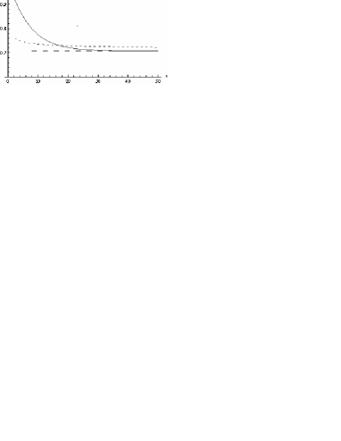
Figure 1: Fidelity (with respect to the Bell state $|00\rangle-|11\rangle$) as a function of time for a two-qubit system interacting with its environment via a QND interaction. The bold curve corresponds to a finite temperature and no squeezing ($T=4,\alpha=0$); the small-dashed curve corresponds to zero temperature but finite squeezing ($T=0,\alpha=2$); the large-dashed curve corresponds to finite temperature and squeezing ($T=4,\alpha=2$). For sufficiently large time, the fidelity approaches $1/\sqrt{2}\approx 0.707$.

VI Characterization of Mixed State Entanglement through a Probability Density Function

As mentioned in the introduction, it is important to determine the entanglement in the two qubit system, if it is to be of utility in quantum information processing. There is, however, no straightforward way of determining the entanglement when the system is in a mixed state since, as is well known, entanglement, as an observable, cannot be represented by a linear hermitian operator. Indeed, it is impossible to capture the information on the entanglement in a mixed state by a single parameter bd96 , notwithstanding the fact that useful benchmarks such as concurrence and negativity exist . Thus , for instance, negativity and concurrence are not relative monotones.

For this reason, we employ a recently proposed description of MSE via a probability density function. We also determine the concurrence (negativity for a state can never exceed its concurrence), and show it along with the PDF, for comparison, and to display the extent to which it captures the information on the entanglement in the state.

Here we briefly recapitulate the characterization of mixed state entanglement (MSE) through a PDF as developed in br08 . The basic idea is to express the PDF of entanglement of a given system density matrix (in this case, a two-qubit) in terms of a weighted sum over the PDF’s of projection operators spanning the full Hilbert space of the system density matrix. Consider first a system in a state which is a projection operator of dimension $d$. The pure states correspond to $d=1$, and the completely mixed states to $d=4$. The PDF of a system in a state which is a projection operator $\rho=\frac{1}{M}\Pi_{M}$ of rank $M$ is defined as:

$${\cal P}_{\Pi_{M}}({\cal E})=\frac{\int d{\cal H}_{\Pi_{M}}\delta({\cal E}_{\psi}-{\cal E})}{\int d{\cal H}_{\Pi_{M}}},$$ (58)

where $\int d{\cal H}_{\Pi_{M}}$ is the volume measure for ${\cal H}_{\Pi_{M}}$, which is the subspace spanned by $\Pi_{M}$. The volume measure is determined by the invariant Haar measure associated with the group of automorphisms of $\int d{\cal H}_{\Pi_{M}}$, modulo the stabilizer group of the reference state generating ${\cal H}_{\Pi_{M}}$. Thus for a one dimensional projection operator, representing a pure state, the group of automorphisms consists of only the identity element and the PDF is simply given by the Dirac delta. Indeed, if $\rho=\Pi_{1}\equiv|\psi\rangle\langle\psi|$, the PDF has the form ${\cal P}_{\rho}({\cal E})=\delta({\cal E}-{\cal E}_{\psi})$ thereby resulting in the description of pure state entanglement, as expected, by a single number. The entanglement density of a system in a general mixed state $\rho$ is given by resolving it in terms of nested projection operators with appropriate weights as

$$\rho = (\lambda_{1}-\lambda_{2})\Pi_{1}+(\lambda_{2}-\lambda_{3})\Pi_{2}+.......(\lambda_{N-1}-\lambda_{N})\Pi_{N-1}+\lambda_{N}\Pi_{N}$$ (59)

$$\equiv \sum_{M=1}^{N}\Lambda_{M}\Pi_{M},$$

where the projections are $\Pi_{M}=\sum_{j=1}^{M}|\psi_{j}\rangle\langle\psi_{j}|$, with $M=1,2,...,N$ and the eigenvalues $\lambda_{1}\geq\lambda_{2}\geq....$, i.e., the eigenvalues are arranged in a non-increasing fashion. Thus the PDF for the entanglement of $\rho$ is given by

$${\cal P}_{\rho}({\cal E})=\sum_{M=1}^{N}\omega_{M}{\cal P}_{\Pi_{M}}({\cal E}),$$ (60)

where the weights of the respective projections ${\cal P}_{\Pi_{M}}({\cal E})$ are given by $\omega_{M}=\Lambda_{M}/\lambda_{1}$. For a two qubit system, the density matrix would be represented as a nested sum over four projection operators, $\Pi_{1}$, $\Pi_{2}$, $\Pi_{3}$, $\Pi_{4}$ corresponding to one, two, three and four dimensional projections, respectively, with $\Pi_{1}$ corresponding to a pure state and $\Pi_{4}$ corresponding to a a uniformly mixed state, is a multiple of the identity operator. The most interesting structure is present in $\Pi_{2}$, the two-dimensional projection, which is characterized by three parameters, viz. ${\cal E}_{cusp}$, the entanglement at which the PDF diverges, ${\cal E}_{max}$, the maximum entanglement allowed and ${\cal P}_{2}({\cal E}_{max})$, the PDF corresponding to ${\cal E}_{max}$. The three dimensional projection $\Pi_{3}$ is characterized by the parameter ${\cal E}_{\perp}$, which parametrizes a discontunity in the entanglement density function curve. By virtue of the convexity of the sum over the nested projections (59), it can be seen that the concurrence of any state $\rho$ is given by the inequality ${\cal C}_{\rho}\leq(\lambda_{1}-\lambda_{2}){\cal C}_{\Pi_{1}}+(\lambda_{2}-\lambda_{3}){\cal C}_{\Pi_{2}}$. Thus while the concurrence for a three and four dimensional projection is identically zero, through the PDF one is able to make a statement about the entanglement content of states which span these spaces. Also, as pointed out in br08 , in the case of NMR quantum computation, concurrence and negativity are zero, whereas the PDF is able to elucidate the role of entanglement utilized by the NMR operations. These features as well as the fact that the PDF (60) enables us to study entanglement of a physical state by exploiting the richness inherent in the subspaces spanned by the system Hilbert space makes the PDF an attractive statistical and geometric characterization of entanglement. We provide an explicit illustration of this in the next section.

VII Entanglement analysis

In this section, we will study the development of entanglement in the two qubit system, both for the localized as well as the collective decoherence model. Recall that concurrence ww98 is defined as

$${\cal C}=\max(0,\sqrt{\lambda_{1}}-\sqrt{\lambda_{2}}-\sqrt{\lambda_{3}}-\sqrt{\lambda_{4}}),$$ (61)

where ${\lambda_{i}}$ are the eigenvalues of the matrix

$$R=\rho\tilde{\rho},$$ (62)

with $\tilde{\rho}=\sigma_{y}\otimes\sigma_{y}\rho^{*}\sigma_{y}\otimes\sigma_{y}$ and $\sigma_{y}$ is the usual Pauli matrix. ${\cal C}$ is zero for unentangled states and one for maximally entangled states. In the above expression, it is implicitly assumed that $\rho$ is expressed in a seperable basis.

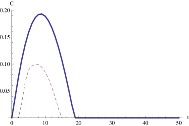
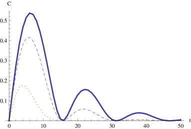
Figure 2: Concurrence ${\cal C}$ (61) as a function of time of evolution $t$ at $T=5.0$ and bath squeezing parameter $\alpha$ (17) equal to $0$, $0.5$, $1.0$, corresponding to the bold, dashed and dotted curves, respectively. Figure (a) refers to the localized decoherence model and (b) the collective decoherence model.

In figure (2 (a)), we plot the concurrence (61) with respect to time for the case of the localized decoherence model, while figure (2 (b)) depicts the temporal behavior of concurrence for the collective decoherence model, for different bath squeezing parameters. In all figures in this article, $kr_{12}$ is set equal to 1.1 for the localized decoherence model and 0.05 for the collective model. It is clearly seen from the figures that the two qubit system is initially unentangled, but with time there is a build up of entanglement between them as a result of their interaction with the bath. Also the entanglement builds up more quickly in the collective decoherence model when compared to the localized model. This is expected as the effective interaction between the two qubits is stronger in the collective case. Another interesting feature that can be inferred from figure (2 (a)) is the phenomena of entanglement birth and death ye09 in the localized decoherence model. Figure (2 (b)) exhibits entanglement death followed by revival, in the collective decoherence model. It is clear from the figures that bath squeezing retards the dynamical generation of entanglement. However, interestingly, it is observed that the disentanglement time is the same for different bath squeezing parameters, as in figure (2 (b)), while it varies for the independent decoherence model, figure (2 (a)). This indicates a kind of robustness of the phenomena of disentanglement with respect to bath squeezing, in the collective regime.

There have been a number of investigations in the phenomena of entanglement sudden death and revival. In ye06 a study of entanglement sudden death and revival was made between two isolated atoms each in its own lossless Jaynes-Cummings cavity, while in ye07 the evolution of entanglement was studied via information exchange between subsystems rather than decoherence. Thus these studies revealed features of the dynamics of entanglement generation in the absence of decoherence. In another study ft06 was revealed the interesting effect that irreversible spontaneous decay, due to interaction with a vacuum bath, can have on the revival of entanglement between two qubits with the collective decoherence regime being most conducive to the revival of entanglement. Even though this work involved a dissipative system-bath interaction, this conclusion is supported here, for QND interactions, as the generation of entanglement is seen to be much more effective in the collective regime when compared to the independent one. The effect of non-Markovian influences, due to a dissipative interaction, on the dynamics of entanglement between two qubits was studied in bc08 for the localized decoherence model and in mp08 for the collective regime. Here our study concentrates on QND interactions and localized as well as collective regimes are treated under a common footing.

Now we take up the issue of entanglement from the perspective of the PDF as in Eq. (60). In figures (3 (a)) and (b), we plot the weights $\omega_{1}$, $\omega_{2}$, $\omega_{3}$ and $\omega_{4}$ (60) of the entanglement densities of the projection operators of the various subspaces which span the two qubit Hilbert space with respect to $T$ for the localized and collective decoherence models, respectively. As can be seen from both the figures , with increase in temperature $T$, the weight $\omega_{1}$, depicting the pure state component monotonically decreases, while the other weights start from zero at $T=0$ and increase. Eventually, the weight $\omega_{4}$ depicting a maximally mixed state would be expected to dominate, though for the parameter range used in the plots, this feature is not seen. This feature of the dynamics of the reduced two-qubit system, specially in the case of the collective decoherence model, has an interesting application which will be discussed in detail in Section VIII where it will be seen to obey an effective temperature dependent Hamiltonian, bringing out the persistence of entanglement even at finite temperatures. In the case of the collective decoherence model, the weights $\omega_{2}$ and $\omega_{3}$ have a greater growth than that for the localized decoherence model, depicting the greater entanglement development in the collective model as is also borne out by the concurrence plots in figure (2).

Figure 3: The weights (60) as a function of $T$, with an evolution time $t=5$ and bath squeezing parameter $\alpha$ (17) equal to $0.2$. Figure (a) refers to the localized decoherence model and (b) the collective decoherence model. In both the figures, the bold curve corresponds to the weight $\omega_{1}$, while the large-dashed, small-dashed and dotted curves correspond to the weights $\omega_{2}$, $\omega_{3}$ and $\omega_{4}$, respectively.

As explained in Section VI, the characterization of MSE for a two qubit system via the PDF involves the distribution functions of four projection operators, $\Pi_{1}$, $\Pi_{2}$, $\Pi_{3}$, $\Pi_{4}$ corresponding to one, two, three and four dimensional projections, respectively. These will be represented here as ${\cal P}_{1}({\cal E})$, ${\cal P}_{2}({\cal E})$, ${\cal P}_{3}({\cal E})$ and ${\cal P}_{4}({\cal E})$, respectively. Also, as discussed above, ${\cal P}_{4}({\cal E})$ would be universal for the two qubit density matrices and would involve the Haar measure on $SU(4)$ br08 ; tbs02 .

Consideration of the ${\cal P}_{2}({\cal E})$ and ${\cal P}_{3}({\cal E})$ density functions for some representative states of the two qubit system, both for the localized as well as collective decoherence models, enables us to compare the entanglement in the respective subspaces of the system Hilbert space. The details of these density functions for different parameters, pertaining to the two-qubit reduced dynamics, have been presented in entqnd09 .

Figures (4 (a)) and (b) give the full density function ${\cal P}(\cal E)$ for the localized and collective decoherence models, respectively, with a bath evolution time $t=10.0$ and $T=50.0$. For these conditions, the value of concurrence (61) is 0, which would indicate a complete breakdown of entanglement. This would be expected as with the increase in the bath temperature $T$, the effect of entanglement would be destroyed quickly. This is partially borne out by the fact that for this case ${\cal C}_{\Pi_{2}}=0$. However, as seen from figure (4 (b)), the PDF for the full density function still exhibits a rich entanglement structure, coming principally from the contributions from the one and three dimensional projections. In contrast, figure (4 (a)), for the localized decoherence model, exhibits the Haar measure on $SU(4)$ and thus represents a maximally mixed state.

Figures (5) represents the full density function ${\cal P}(\cal E)$ for the localized decoherence model with an evolution time $t=10.0$, $T=20.0$ and bath squeezing parameter $\alpha$ equal to $0.2$, figure (a), and equal to $0$ in figure (b). This case is interesting since it is analogous to that discussed in br08 for NMR quantum computation where concurrence would be zero, and the excess of entangled states over the unpolarized background (exhibited by the uniform distribution coming from the density function $\Pi_{4}$, related to the fourth dimensional projection) is exploited as a resource allowing for non-trivial gate operations, thus depicting pseudopure states over the four dimensional background, with the excess being the “deviation density matrix”. A comparison of the two figures shows that the generation of entanglement is greater for the case of zero bath squeezing, as in figure (b), when compared to the case of finite bath squeezing, figure (a).

Figure 4: The full density function ${\cal P}({\cal E})$ (60) with respect to the entanglement ${\cal E}$ for an evolution time $t=10.0$, $T=50.0$ and bath squeezing parameter $\alpha$ equal to $0.2$. Figure (a) refers to the localized decoherence model and (b) to the collective decoherence model.

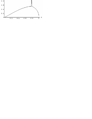
Figure 5: The full density function ${\cal P}({\cal E})$ (60) with respect to the entanglement ${\cal E}$ for the localized decoherence model with an evolution time $t=10.0$, $T=20.0$ and bath squeezing parameter $\alpha$ equal to $0.2$ (figure (a)) and $0$ (figure (b)).

VIII Effective temperature dependent dynamics in the collective decoherence model: a brief discussion

In a QND $S-R$ interaction, the reduced density matrix of the system does not approach a unique distribution asymptotically bg07 . It turns out that the PDF for the full density function (for the collective decoherence model) exhibits a rich entanglement structure, coming principally from the contributions from the one and three dimensional projections which carry equal weights. This feature is seen to persist for higher temperatures and evolution times, for the collective decoherence model, with the weights of the subspaces spanned by the four projection operators of the PDF remaining intact. From this emerges the fact that for the collective decoherence model, studied here, as the effect of the bath on the system increases, the PDF instead of becoming uniform, as expected, gets distributed between the subspaces spanned by the one and three dimensional projection operators suggesting a tendency of the system to resist randomization. We may ask if the description of the mixed state entanglement in terms of the probability density function which we employ here can throw, as a nontrivial application, light on the effective dynamics of the two qubit system. It has been seen in earlier studies that such a state of affairs would be encountered if the effect of the bath is not a counterpart of the collision term (in a Boltzmann equation), but is more like a Vlasov term, causing long range mean field contributions ce94 . We analyse our system in detail below.

Indeed, from the numerical results, it is not difficult to see that the effect of the bath can be mapped to a $T$ dependent effective hamiltonian whose energy eigenvalues scale with temperature. The eigenstates are given by the standard Bell states with the ground state being $|B_{1}\rangle=\frac{1}{\sqrt{2}}(|01\rangle+|10\rangle)$ while the orthogonal singlet state ($|B_{4}\rangle=\frac{1}{\sqrt{2}}(|01\rangle-|10\rangle)$) is the highest energy state, and is practically decoupled (with no population). The next excited state is degenerate, with two Bell states ($|B_{2}\rangle=\frac{1}{\sqrt{2}}(|00\rangle-|11\rangle)$, $|B_{3}\rangle=\frac{1}{\sqrt{2}}(|00\rangle+|11\rangle)$) spanning the two dimensional subspace. Thus it follows that the effective temperature dependent hamiltonian is given by

$$H_{\rm eff}=\sum^{4}_{i=1}E_{i}(\beta)|B_{i}\rangle\langle B_{i}|,$$

where $|B_{1}\rangle$, $|B_{2}\rangle\langle B_{2}|+|B_{3}\rangle\langle B_{3}|=|00\rangle\langle 00|+|11\rangle\langle 11|$ and $|B_{4}\rangle$ are the Bell states, as defined above, with eigenvalues $\lambda_{1}=0.5$, $\lambda_{2}=\lambda_{3}=0.25$ and $\lambda_{4}\approx 0$, respectively. Since the Bell states are completely entangled, the effective hamiltonian has no linear terms in the qubit polarizations and has the form

$$H_{eff}\sim\frac{\ln(2)}{2\beta}(1-(-\sigma_{x}^{(1)}\sigma_{x}^{(2)}+\sigma_{y}^{(1)}\sigma_{y}^{(2)}-\sigma_{z}^{(1)}\sigma_{z}^{(2)}))+\frac{\ln(4)}{\beta}(\frac{1}{2}+2\sigma_{z}^{(1)}\sigma_{z}^{(2)}),$$ (63)

in writing which the singlet term has been dropped, as it is energetically very far separated from the other three levels. The above analysis places in perspective the surprising result that although the system is evolving, through the effective Hamiltonian, the entanglement density function remains practically restricted to the 3-dimensional subspace, with a large contribution from a Bell state, as the signal with the 3-dimensional background acting as noise. The restriction of the effective dynamics from four to three levels is also seen in the case of two qubit evolution via a dissipative $S-R$ interaction with a thermal bath initially at $T=0$ ft02 , for the collective decoherence model. However, there the reason for it is simply given by the fact that for the above conditions, the coupling term connecting one of the levels to the others goes to zero, thereby reducing the dynamics to that between three levels.

An interesting analog of the discussion in this Section comes in the work presented in hn03 . There it was shown by the authors that for the scenario where there exists a system consisting of three subsystems with the first and the third interacting with each other via their interactions with the mediating second subsystem, a signature of entanglement between the first and the third subsystems is the degeneracy in the ground state of the system. Here we have a similar situation with the two qubits interacting with a bath which in turn mediates the inter-qubit interaction. From our effective Hamiltonian $H_{eff}$, we see that the first excited state (not the ground state), spanned by the Bell states $|B_{2}\rangle$ and $|B_{3}\rangle$, is degenerate and the system exhibits a strong entanglement even at finite temperatures. Another work by the same authors on02 , studied the persistence of mixed state entanglement at finite $T$. This would be important as quantum effects can be expected to dominate in regions where entanglement is nonzero. They considered the transverse Ising model and studied the two-site entanglement, using concurrence as the entanglement measure, and found appreciable entanglement in the system at finite $T$ above the ground state energy gap, one of their motivations being the influence of nearby critical points to the finite $T$ entanglement. The persistence of entanglement in a two-qubit system interacting with the bath via a purely dephasing interaction (QND) would suggest a broad applicability of these concepts, thereby highlighting the interconnection of ideas of quantum information to quantum statistical mechanics.

IX Conclusions

In this article, we have analyzed in detail the dynamics of entanglement in a two-qubit system interacting with its environment via a purely dephasing QND $S-R$ interaction. The system and reservoir are initially assumed to be separable with the reservoir being in an initial squeezed thermal state. Since the resulting dynamics becomes mixed, in order to analyze the ensuing entanglement, we have made use of a recently introduced measure of mixed state entanglement via a PDF. This enables us to give a statistical and geometrical characterization of entanglement.

After developing the general dynamics of $N$ qubits interacting with their bath (reservoir) via a QND $S-R$ interaction, we specialized to the two-qubit case for applications. Due to the position dependent coupling of the qubits with the bath, the dynamics could be naturally divided into a localized and collective decoherence regime, where in the collective decoherence regime, the qubits are close enough to feel the bath collectively. We analyzed the open system dynamics of the two qubits, both for the localized as well as the collective regimes and saw that in the collective regime, there emerges the possibility of a decoherence-free subspace for the case of zero bath squeezing. Interestingly, the dynamics was found to obey a non-trivial spin-flip symmetry operation. The existence of the nontrivial spin-flip symmetry would explain the emergence of a decoherence-free subspace (DFS) dfs , thereby providing a concrete instance of a DFS. We made an application of the two-qubit system to a simplified model of a quantum repeater, which can be adapted for quantum communication over long distances.

We then made an analysis of the two-qubit entanglement for different bath parameters. We analyzed both concurrence as well as the PDF by finding the entanglement content of the various subspaces that span the two-qubit Hilbert space. The analysis of concurrence revealed the interesting feature of so called entanglement birth and death in the localized decoherence model, while the collective model saw a subsequent revival of entanglement. Reservoir squeezing was seen to hinder the generation of entanglement, though the process of disentanglement, as seen from concurrence, was robust, in the collective regime, against the effects of squeezed bath. Although the PDF agrees qualitatively in its predictions with concurrence, it is able to extract more information out of the system as a result of its statistical-geometrical nature. Thus we were able to consider an example analogous to NMR quantum computation, wherein the concurrence would be zero, and the excess of entangled states over the unpolarized background is exploited as a resource allowing for non-trivial quantum information processing. For the collective decoherence model the PDF for the full density function exhibits a rich entanglement structure, coming principally from the contributions from the one and three dimensional projections which carry equal weights thereby suggesting a tendency of the system to resist randomization. This feature is seen to persist even for higher temperatures and evolution times with the weights of the subspaces spanned by the four projection operators of the PDF remaining intact. The probability density description of entanglement sheds light on the underlying dynamics thereby enabling us to give an effective $T$ dependent dynamics in the collective decoherence regime. A comparison of this with some related works suggests the applicability of quantum information theoretic ideas to quantum statistical mechanical systems.

- (1) W. H. Louisell, Quantum Statistical Properties of Radiation (John Wiley and Sons, 1973).
- (2) A. O. Caldeira and A. J. Leggett, Physica A 121, 587 (1983).
- (3) W. H. Zurek, Phys. Today 44, 36 (1991); Prog. Theor. Phys. 87, 281 (1993).
- (4) G. L. Ingold, arXiv:0208026.
- (5) S. Banerjee and R. Ghosh, J. Phys. A: Math. Theo. 40, 13735 (2007); eprint quant-ph/0703054.
- (6) V. B. Braginsky, Yu. I. Vorontsov and K. S. Thorne, Science 209, 547 (1980).
- (7) V. B. Braginsky and F. Ya. Khalili, in Quantum Measurements, edited by K. S. Thorne (Cambridge University Press, Cambridge, 1992).
- (8) D. F. Walls and G. J. Milburn, Quantum Optics (Springer, Berlin, 1994).
- (9) W. H. Zurek, in The Wave-Particle Dualism, edited by S. Diner, D. Fargue, G. Lochak and F. Selleri (D. Reidel Publishing Company, Dordrecht, 1984).
- (10) C .M. Caves, K. D. Thorne, R. W. P. Drever, V. D. Sandberg and M. Zimmerman, Rev. Mod. Phys. 52, 341 (1980).
- (11) M. F. Bocko and R. Onofrio, Rev. Mod. Phys. 68, 755 (1996).
- (12) E. Andersson and D. K. L. Oi, Phys. Rev. A 77, 0520104 (2008).
- (13) C. J. Myatt, B. E. King, Q. A. Turchette, C. A. Sackett, et al., Nature 403, 269 (2000).
- (14) Q. A. Turchette, C. J. Myatt, B. E. King, C. A. Sackett, et al., Phys. Rev. A 62, 053807 (2000).
- (15) G. J. Pryde, J. L. O’Brien, A. G. White, et al., Phys. Rev. Lett. 92, 190402 (2004); J. L. O’Brien, G. J. Pryde, A. G. White, et. al., Nature 426, 264 (2003).
- (16) R. Onofrio and L. Viola, Phys. Rev. A 58, 69 (1998).
- (17) J. S. Bell, Physics 1, 195 (1964).
- (18) M. Nielsen and I. Chuang, Quantum Computation and Quantum Information (Cambridge University Press, Cambridge, 2000).
- (19) P. Shor, SIAM Journal of Computing 26, 1484 (1997); L. K. Grover, Phys. Rev. Lett. 79, 325 (1997).
- (20) S. Calderbank and P. Shor, Phys. Rev. A̱ 54, 1098 (1996); A. Steane, Proc. Roy. Soc., London, Ser. A 452, 2551 (1996).
- (21) A. Beige, D. Braun, B. Tregenna and P. L. Knight, Phys. Rev. Lett. 85, 1762 (2000).
- (22) M. Fleischhauer, S. F. Yelin and M. D. Lukin, Opt. Commun. 179, 395 (2000).
- (23) S. Schneider and G. J. Milburn, Phys. Rev. A 65, 042107 (2002).
- (24) H.-P. Breuer and F. Petruccione, The Theory of Open Quantum Systems (Oxford University Press 2002).
- (25) H. Carmichael, An Open Systems Approach to Quantum Optics (Springer 1993).
- (26) M. P. Almeida, F. de Melo, M. Hor-Meyll, A. Salles, et al., Science 316, 579 (2007); A. Salles, F. Melo, M. P. Almeida, M. Hor-Meyll, et al., arXiv:0804.4556.
- (27) R. Srikanth and S. Banerjee, Phys. Rev. A 77, 012318 (2008); arXiv:0707.0059.
- (28) I. Bengtsson and K. Zyczkowski, Geometry of Quantum States: An Introduction to Quantum Entanglement (Cambridge University Press, Cambridge, 2006).
- (29) C. H. Bennett, D. P. DiVincenzo, J. A. Smolin and W. K. Wootters, Phys. Rev. A 54, 3824 (1996).
- (30) W. K. Wootters, Phys. Rev. Lett. 80, 2245 (1998).
- (31) F. Mintert, A. R. R. Carvalho, M. Kus and A. Buchleitner, Phys. Reports 415, 207 (2005).
- (32) R. F. Werner, Phys. Rev. A 40, 4277 (1989).
- (33) S. Bhardwaj and V. Ravishankar, Phys. Rev. A 77, 022322 (2008).
- (34) H.-J. Briegel, W. Dür, J. I. Cirac and P. Zoller, Phys. Rev. Lett. 81, 5932 (1998); W. Dür, H.-J. Briegel, J. I. Cirac, and P. Zoller, Phys. Rev. A 59, 169 (1999).
- (35) C. H. Bennett, G. Brassard, S. Popescu, B. Schumacher et al., Phys. Rev. Lett. 76,722 (1996).
- (36) J. H. Reina, L. Quiroga and N. F. Johnson, Phys. Rev. A 65, 032326 (2002).
- (37) S. Banerjee, J. Ghosh and R. Ghosh, Phys. Rev. A 75, 062106 (2007); eprint quant-ph/0703055.
- (38) S. Banerjee and R. Srikanth, Eur. Phys. J. D 46 335 (2008); eprint quant-ph/0611161.
- (39) C. M. Caves and B. L. Schumacher, Phys. Rev. A 31, 3068 (1985); B. L. Schumacher and C. M. Caves, Phys. Rev. A 31, 3093 (1985).
- (40) C. H. Bennett, G. Brassard, C. Crépeau, R. Josza, A. Peres and W. K. Wootters, Phys. Rev. Lett. 70, 1895 (1993).
- (41) T. Yu and J. H. Eberly, Science 323, 598 (2009).
- (42) M. Yonac, T. Yu and J. H. Eberly, J. Phys. B: At. Mol. Opt. Phys. 39, S621 (2006).
- (43) M. Yonac, T. Yu and J. H. Eberly, J. Phys. B: At. Mol. Opt. Phys. 40, S45 (2007).
- (44) Z. Ficek and R. Tanas, Phys. Rev. A 74, 024304 (2006).
- (45) B. Bellomo, R. Lo Franco and G. Compagno, Phys. Rev. A 77, 032342 (2008).
- (46) S. Maniscalco, F. Francica, R. L. Zaffino, N. L. Gullo and F. Plastina, Phys. Rev. Lett. 100, 090503 (2008).
- (47) T. E. Tilma, M. Byrd and E. C. G. Sudarshan, J. Phys. A: Math. Gen. 35, 9255 (2002).
- (48) S. Banerjee, V. Ravishankar and R. Srikanth, arXiv:0810.5034.
- (49) E. Carlen, R. Esposito, J. L. Lebowitz, R. Marra and A. Rokhlenko, Preprint (1994) (unpublished).
- (50) Z. Ficek and R. Tanaś, Physics Reports, 372, 369 (2002).
- (51) H. L. Haselgrove, M. A. Nielsen and T. J. Osborne, arXiv:quant-ph/0308083.
- (52) T. J. Osborne and M. A. Nielsen, arXiv:quant-ph/0202162.
- (53) P. Zanardi and M. Rasetti, Phys. Rev. Lett. 79, 3306 (1998); L. M. Duan and G. C. Guo, Phys. Rev. A 57, 737 (1998); D. A. Lidar, I. L. Chuang and K. B. Whaley, Phys. Rev. Lett. 89, 2594 (1998); D. A. Lidar and K. B. Whaley, Irreversible Quantum Dynamics, F. Benatti and R. Floreanini (eds.) Springer Lecture Notes in Physics 622 (Berlin 2003).