PHANTOM COSMOLOGY BASED ON PT SYMMETRY

Abstract

We consider the PT symmetric flat Friedmann model of two scalar fields with positive kinetic terms. While the potential of one (“normal”) field is taken real, that of the other field is complex. We study a complex classical solution of the system of the two Klein-Gordon equations together with the Friedmann equation. The solution for the normal field is real while the solution for the second field is purely imaginary, realizing classically the “phantom” behavior. The energy density and pressure are real and the corresponding geometry is well-defined. The Lagrangian for the linear perturbations has the correct potential signs for both the fields, so that the problem of stability does not arise. The background dynamics is determined by an effective action including two real fields one normal and one “phantom”. Remarkably, the phantom phase in the cosmological evolution is transient and the Big Rip never occurs. Our model is contrasted to well-known quintom models, which also include one normal and one phantom fields.

1 Introduction

Complex (non-Hermitian) Hamiltonians with PT symmetry have been vigorously investigated in quantum mechanics and quantum field theory[1]. A possibility of applications to quantum cosmology has been pointed out in Ref. PT-cosm. In the present contribution we mainly focus attention on complex field theory. We explore the use of a particular complex scalar field Lagrangian, whose solutions of the classical equations of motion provide us with real physical observables and well-defined geometric characteristics.

The interest of our approach is related to its focusing on the intersection between two important fields of research: PT symmetric quantum theory and the cosmology of dark energy models.

As is well known the discovery of cosmic acceleration[4] has stimulated an intensive study of models of dark energy[5] responsible for the origin of this phenomenon. Dark energy is characterized by a negative pressure whose relation to the energy density $w=p/\varepsilon$ is less than $-1/3$. Moreover, if this relation happens to be less than $-1$ such kind of dark energy is called “phantom” dark energy[6]. The condition $w>-1$ is called the dominant energy condition. The breakdown of this condition implies the so called super-acceleration of cosmological evolution, which in some models culminates approaching a new type of cosmological singularity called Big Rip[7]. While the cosmological constant ($w=-1$) is still a possible candidate for the role of dark energy, there are observations giving indications in favor of the models where the equation of state parameter $w$ not only changes with time, but would be less than $-1$ no[8]. A standard way to introduce the phantom energy is to consider a scalar field with the negative sign of the kinetic energy term, usually called “phantom” scalar field. However such a model has been reasonably criticized insofar as it is unstable with respect to linear perturbations[9]. Constraints on phantom particles have been discussed in Ref. crit1.

In the present paper we propose a cosmological model inspired by PT symmetric theory[1], choosing potentials so that the equations of motion have classical phantom solutions for homogeneous and isotropic universe. Meanwhile quantum fluctuations have positive energy density and this ensures the stability around a classical background configuration. Thus our study is inspired by samples of potentials providing the real energy spectrum bounded from below[1, 11, 12, 13, 14].

The PT symmetric approach to the extension of quantum physics consists in the weakening of the requirement of Hermiticity, while keeping all the physical observables real. It was shown that the axioms of quantum theory are maintained if the complex extension preserves (C)PT symmetry[14]. There have also been some attempts to apply the PT symmetric formalism to cosmology[2, 3]. We do not enter into the discussion about the equivalence between the PT symmetric theories and Hermitian theories with non-local Hamiltonians. The reader is refereed to review papers in Refs. Bender-review,mostaf.

We consider the complex extension of matter Lagrangians requiring the reality of all the physically measurable quantities and the well-definiteness of geometrical characteristics. We would like to underline here, that we work with real space-time manifolds. The attempts to use complex manifolds for studying the problem of dark energy in cosmology were undertaken in Refs. complex-man.

We start with the flat Friedmann model of two scalar fields with positive kinetic terms. The potential of the model is additive. One term of the potential is real, while the other is complex and PT symmetric. We find a classical complex solution of the system of the two Klein-Gordon equations together with the Friedmann equation. The solution for one field is real (the “normal” field) while the solution for the other field is purely imaginary, realizing classically the “phantom” behavior. Moreover, the effective Lagrangian for the linear perturbations has the correct potential signs for both the fields, so that the problem of stability does not arise. However, the background (homogeneous Friedmann) dynamics is determined by an effective action including two real fields one normal and one phantom. As a byproduct, we notice that the phantom phase in the cosmological evolution is inevitably transient. The number of phantom divide line (PDL) crossings, (i.e. events such that the ratio $w$ between pressure and energy density passes through the value $-1$) can be only even and the Big Rip never occurs. The avoidance of Big Rip singularity constitutes an essential difference between our model and well-known quintom models, including one normal and one phantom fields[17]. The other differences will be discussed in more detail later.

The paper is organized as follows: in Sec. 2 we describe the cosmological model we want to analyze, together with a brief explanation of PT symmetric quantum mechanics; in Sec. 3 we present the results of the qualitative analysis and of the numerical simulations for the dynamical system under consideration; conclusion and perspectives are presented in the last section.

2 Phantom and stability

We shall study the flat Friedmann cosmological model described by the metric

$$ds^{2}=dt^{2}-a^{2}(t)dl^{2},$$

where $a(t)$ is the cosmological radius of the universe. The dynamics of the cosmological evolution is characterized by the Hubble variable

$$h\equiv\frac{\dot{a}}{a},$$

which satisfies the Friedmann equation

$$h^{2}=\varepsilon,$$ (1)

where $\varepsilon$ is the energy density of the matter populating the universe.

We consider the matter represented by scalar fields with complex potentials. Namely, we shall try to find a complex potential possessing the solutions of classical equations of motion which guarantee the reality of all observables. Such an approach is inspired by the quantum theory of the PT symmetric non-Hermitian Hamiltonians, whose spectrum is real and bounded from below. Thus, it is natural for us to look for Lagrangians which have consistent counterparts in the quantum theory.

Let’s elucidate how the phantom-like classical dynamics arises in such Lagrangians and for this purpose choose the one-dimensional PT symmetric potential of anharmonic oscillator $V^{(2+\epsilon)}(q)=\lambda q^{2}(iq)^{\epsilon},\ 0<\epsilon\leq 2$ which has been proven[1, 11, 12, 14] to possess a real energy spectrum bounded from below. For illustration, we restrict ourselves with $\epsilon=2,V^{(4)}(q)=-\lambda q^{4}$. The classical dynamics for real coordinates $q(t)$ offers the infinite motion with increasing speed and energy or, in the quantum mechanical language, indicates the absence of bound states and unboundness of energy from below. However, just there is a more consistent solution which, at the quantum level, provides the real discrete energy spectrum, certainly, bounded from below. It has been proven, first, by means of path integral[11] and, further on, by means of the theory of ordinary differential equations[18]. In fact, this classically “crazy” potential on a curve in the complex coordinate plane generates the same energy spectrum as a two-dimensional quantum anharmonic oscillator $V^{(4)}(\vec{q})=\lambda(q_{1}^{4}+q_{2}^{4})/4$ with real coordinates $q_{1,2}$ in the sector of zero angular momentum[11]. Although the superficially unstable anharmonic oscillator is well defined on the essentially complex coordinate contour any calculation in the style of perturbation theory (among them the semiclassical expansion) proceeds along the contour with a fixed complex part (corresponding to a ”classical” solution) and varying unboundly in real direction. In particular, the classical trajectory for $V^{(4)}(q)$ with keeping real the kinetic, $(\dot{q})^{2}$ and potential, $-\lambda q^{4}(t)$ energies (as required by its incorporation into a cosmological scenario) can be chosen imaginary,

$$q=i\xi,\quad\ddot{\xi}=-2\lambda\xi^{3},\quad\dot{\xi}^{2}=C-\lambda\xi^{4},\quad C>0$$

which obviously represents a bounded, finite motion with $|\xi|\leq(C/\lambda)^{1/4}$. Such a motion supports the quasi-classical treatment of bound states with the help of Bohr’s quantization. Evidently, the leading, second variation of the Lagrangian around this solution, $q(t)=i\xi(t)+\delta q(t)$ gives a positive definite energy,

$${\cal L}^{(2)}=p(t)\delta\dot{q}(t)-H,\ H=\frac{1}{4}p^{2}(t)+12\xi^{2}(t)(\delta q(t))^{2}$$

realizing the perturbative stability of this anharmonic oscillator in the vicinity of imaginary classical trajectory. It again reflects the existence of positive discrete spectrum for this type of anharmonicity. However the classical kinetic energy $-\dot{\xi}^{2}$ is negative, i.e. it is phantom-like.

In a more general, Quantum Field Theory setting let us consider a non-Hermitian (complex) Lagrangian of a scalar field

$$L=\frac{1}{2}\partial_{\mu}\phi\partial^{\mu}\phi^{*}-V(\phi,\phi^{*}),$$ (2)

with the corresponding action,

$$S(\phi,\phi^{*},g)=\int\,d^{4}x\sqrt{-|\!|g|\!|}(L+\frac{1}{6}R(g)),$$ (3)

where $|\!|g|\!|$ stands for the determinant of a metric $g^{\mu\nu}$ and $R(g)$ is the scalar curvature term and the Newton gravitational constant is normalized to $3/8\pi$ to simplify the Friedmann equations further on.

We employ potentials $V(\Phi,\Phi^{*})$ satisfying the invariance condition

$$(V(\Phi,\Phi^{*}))^{*}=V(\Phi^{*},\Phi),$$ (4)

while the condition

$$(V(\Phi,\Phi^{*}))^{*}=V(\Phi,\Phi^{*}),$$ (5)

is not satisfied. This condition represents a generalized requirement of $(C)PT$ symmetry.

Let’s define two real fields,

$$\phi\equiv\frac{1}{2}(\Phi+\Phi^{*}),\quad\chi\equiv\frac{1}{2i}(\Phi-\Phi^{*}).$$ (6)

Then, for example, such a potential can have a form

$$V(\Phi,\Phi^{*})=\tilde{V}(\Phi+\Phi^{*},\Phi-\Phi^{*})=\tilde{V}(\phi,i\chi),$$ (7)

where $\tilde{V}(x,y)$ is a real function of its arguments. In the last equation one can recognize the link to the so called $(C)PT$ symmetric potentials if to supply the field $\chi$ with a discrete charge or negative parity. When keeping in mind the perturbative stability we impose also the requirement for the second variation of the potential to be a positive definite matrix which, in general, leads to its PT-symmetry[3].

Here, the functions $\phi$ and $\chi$ appear as the real and the imaginary parts of the complex scalar field $\Phi$, however, in what follows, we shall treat them as independent spatially homogeneous variables depending only on the time parameter $t$ and, when necessary, admitting the continuation to complex values .

3 Cosmological solution with classical phantom field

It appears that among known PT symmetric Hamiltonians (Lagrangians) possessing the real spectrum one which is most suitable for our purposes is that with the exponential potential. It is connected with the fact that the properties of scalar field based cosmological models with exponential potentials are well studied[19]. In particular, the corresponding models have some exact solutions providing a universe expanding according to some power law $a(t)=a_{0}t^{q}$. We shall study the model with two scalar fields and the additive potential. Usually, in cosmology the consideration of models with two scalar fields (one normal and one phantom, i.e. with the negative kinetic term) is motivated by the desire of describing the phenomenon of the so called phantom divide line (PDL) crossing. At the moment of the phantom divide line crossing the equation of state parameter $w=p/\varepsilon$ crosses the value $w=-1$ and (equivalently) the Hubble variable $h$ has an extremum. Usually the models using two fields are called “quintom models”[17]. As a matter of fact the PDL crossing phenomenon can be described in the models with one scalar field, provided some particular potentials are chosen[20, 21] or in the models with non-minimal coupling between the scalar field and gravity[22] However, the use of two fields make all the considerations more simple and natural. In this paper, the necessity of using two scalar fields follows from other requirements. We would like to implement a scalar field with a complex potential to provide the effective phantom behavior of this field on some classical solutions of equations of motion. Simultaneously, we would like to have the standard form of the effective Hamiltonian for linear perturbations of this field. The combination of these two conditions results in the fact the background contribution of both the kinetic and potential term in the energy density, coming from this field are negative. To provide the positivity of the total energy density which is required by the Friedmann equation (1) we need the other normal scalar field. Thus, we shall consider the two-field scalar Lagrangian with the complex potential

$$L=\frac{\dot{\phi}^{2}}{2}+\frac{\dot{\chi}^{2}}{2}-Ae^{\alpha\phi}+Be^{i\beta\chi},$$ (8)

where $A$ and $B$ are real, positive constants. This Lagrangian is the sum of two terms. The term representing the scalar field $\phi$ is a standard one, and it can generate a power-law cosmological expansion[19]. The kinetic term of the scalar field $\chi$ is also standard, but its potential is complex. In quantum mechanics dynamical systems like the latter have been studied in the framework of PT symmetric quantum mechanics[1] and, in particular, the exponential potential has been analyzed in great detail in Ref. exponential. The most important feature of this potential is that the spectrum of the corresponding Hamiltonian is real and bounded from below, provided correct boundary conditions are assigned.

Inspired by this fact we are looking for a classical complex solution of the system, including two Klein-Gordon equations for the fields $\phi$ and $\chi$:

$$\ddot{\phi}+3h\dot{\phi}+A\alpha e^{\alpha\phi}=0,$$ (9)

$$\ddot{\chi}+3h\dot{\chi}-iB\beta e^{i\beta\chi}=0,$$ (10)

and the Friedmann equation

$$h^{2}=\frac{\dot{\phi}^{2}}{2}+\frac{\dot{\chi}^{2}}{2}+Ae^{\alpha\phi}-Be^{i\beta\chi}.$$ (11)

The classical solution which we are looking for should provide the reality and positivity of the right-hand side of the Friedmann equation (11). The solution where the scalar field $\phi$ is real, while the scalar field $\chi$ is purely imaginary

$$\chi=i\xi,\quad\xi\ {\rm real},$$ (12)

uniquely satisfies this condition. Moreover, the Lagrangian (8) evaluated on this solution is real as well. This is remarkable because on homogeneous solutions the Lagrangian coincides with the pressure, which indeed should be real.

Substituting the equation(12) into the Friedmann equation (11) we shall have

$$h^{2}=\frac{\dot{\phi}^{2}}{2}-\frac{\dot{\xi}^{2}}{2}+Ae^{\alpha\phi}-Be^{-\beta\xi}.$$ (13)

Hence, effectively we have the Friedmann equation with two fields: one ($\phi$) is a standard scalar field, the other ($\xi$) has the phantom behavior, as we pointed out above. In the next section we shall study the cosmological dynamics of the (effective) system, including (13), (9) and

$$\ddot{\xi}+3h\dot{\xi}-B\beta e^{-\beta\xi}=0.$$ (14)

The distinguishing feature of such an approach rather than the direct construction of phantom Lagrangians becomes clear when one calculates the linear perturbations around the classical solutions. Indeed the second variation of the action for the field $\chi$ gives the quadratic part of the effective Lagrangian of perturbations:

$$L_{eff}=\frac{1}{2}\dot{\delta\chi}^{2}-\frac{1}{2}(\vec{\nabla}(\delta\chi))^{2}-B\beta^{2}e^{i\beta\chi_{0}}(\delta\chi)^{2},$$ (15)

where $\chi_{0}$ is a homogeneous purely imaginary solution of the dynamical system under consideration and $\vec{\nabla}$ stands for spatial gradients . It is easy to see that on this solution, the effective Lagrangian (15) will be real and its potential term has a sign providing the stability of the background solution with respect to linear perturbations as the related Hamiltonian is positive,

$$H_{eff}^{(2)}=\frac{1}{2}{\delta\pi}^{2}+\frac{1}{2}(\vec{\nabla}(\delta\chi))^{2}+B\beta^{2}e^{-\beta\xi_{0}}(\delta\chi)^{2},\quad\delta\pi\Leftrightarrow\delta\dot{\chi}.$$ (16)

The Hamiltonian of the metric perturbations should be naturally added to the above formulae. This Hamiltonian includes two types of terms: bilinear terms in metric perturbations and mixed terms , including both the metric and scalar field perturbations. The part of the second-order action, including terms bilinear in the metric perturbations can be represented in the following form [23, 24]:

$$S_{g,\ g}^{(2)}=\int d^{4}x\Big{\{}\frac{1}{12}A^{2}(\tau)\Big{[}\frac{1}{2}h^{\mu\nu,\rho}h_{\mu\nu,\rho}-h^{\mu\nu}_{,\mu}h^{\rho}_{\nu,\rho}+h^{\mu\nu}_{,\nu}h_{,\mu}-\frac{1}{2}h_{,\mu}h^{,\mu}\Big{]}$$

$$+A(\tau)A^{\prime}(\tau)\Big{[}\frac{1}{6}(h^{\mu\nu}h_{0\nu,\mu}-h^{\mu\nu}_{,\mu}h_{0\nu})+\frac{1}{12}(h^{\mu 0}h_{,\mu}-h^{\mu 0}_{,\mu}h)\Big{]}$$ (17)

$$-\frac{1}{12}(A^{\prime 2}(\tau)+A(\tau)A^{\prime\prime}(\tau))h^{00}h\Big{\}},$$ (18)

where the “prime” means the derivative with respect to conformal time $\tau$ and the background metrics has the form

$$ds^{2}=A^{2}(\tau)(d\tau^{2}-dl^{2}),$$

while the full metric is

$$g_{\mu\nu}(x)=A^{2}(\tau)(\eta_{\mu\nu}+h_{\mu\nu}(x)).$$

The above expression (18) was obtained by the proper integration by parts and taking into account the equations of motion [23, 24]. The only dangerous term here is the last “massive” term, which can be removed by the choice of gauge fixing condition

$$h^{00}=0.$$ (19)

The second-order action, including mixed terms (the metric perturbations and the perturbations of the field $\chi$) has the following form:

$$S^{(2)}_{g,\,\chi}=\int d^{4}xA^{2}(\tau)\left\{\chi^{\prime}\left(\frac{1}{2}h_{,0}-h^{0\mu}_{\;\;,\mu}\right)-\left(\chi^{\prime\prime}+2\frac{A^{\prime}(\tau)}{A(\tau)}\chi^{\prime}\right)h^{00}\right\}\delta\chi,$$ (20)

where again we have used the equation of motion (the Klein-Gordon equation for the field $\chi$. This term (20) appears annoying because it contains the first derivative of the term $Be^{i\beta\chi}$, which is imaginary. However, one can show that by a proper choice of the gauge condition this imaginary term can be eliminated. Indeed, the gauge condition (19) eliminate from (20) the term, proportional to $h^{00}$. Then remains the term proportional to $\chi^{\prime}$ multiplied by the linear combination of the metric perturbations. This combination can be annihilated by the following choice of the second gauge condition:

$$\frac{1}{2}h_{,0}-h^{0\mu}_{\;\;,\mu}=0.$$ (21)

This condition is compatible with the first gauge condition (19). Thus, we have shown that the stability with respect to perturbations in our model can be proved by fixing a proper gauge condition.

Let us list the main differences between our model and quintom models, using two fields (normal scalar and phantom) and exponential potentials[17]. First, we begin with two normal (non-phantom) scalar fields, with normal kinetic terms, but one of these fields is associated to a complex (PT symmetric) exponential potential. Second, the (real) coefficient multiplying this exponential potential is negative. Third, the background classical solution of the dynamical system, including two Klein-Gordon equations and the Friedmann equation, is such that the second field is purely imaginary, while all the geometric characteristics are well-defined. Fourth, the interplay between transition to the purely imaginary solution of the equation for the field $\chi$ and the negative sign of the corresponding potential provides us with the effective Lagrangian for the linear perturbations of this field which have correct sign for both the kinetic and potential terms: in such a way the problem of stability of the our effective phantom field is resolved. Fifth, the qualitative analysis of the corresponding differential equations, shows that in contrast to the quintom models in our model the Big Rip never occurs. The numerical calculations confirm this statement.

In the next section we shall describe the cosmological solutions for our system of equations.

4 Cosmological evolution

First of all notice that our dynamical system permits the existence of cosmological trajectories which cross PDL. Indeed, the crossing point is such that the time derivative of the Hubble parameter

$$\dot{h}=-\frac{3}{2}(\dot{\phi}^{2}-\dot{\xi}^{2})$$ (22)

is equal to zero. We always can choose $\dot{\phi}=\pm\dot{\xi}$, at $t=t_{PDL}$ provided the values of the fields $\phi(t_{PDL})$ and $\xi(t_{PDL})$ are chosen in such a way, that the general potential energy $Ae^{\alpha\phi}-Be^{-\beta\xi}$ is non-negative. Obviously, $t_{PDL}$ is the moment of PDL crossing. However, the event of the PDL crossing cannot happen only once. Indeed, the fact that the universe has crossed phantom divide line means that it was in effectively phantom state before or after such an event, i.e. the effective phantom field $\xi$ dominated over the normal field $\phi$. However, if this dominance lasts for a long time it implies that non only the kinetic term $-\dot{\xi}^{2}/2$ dominates over the kinetic term $\dot{\phi}^{2}/2$ but also the potential term $-B\exp(-\beta\xi)$ should dominate over $A\exp(\alpha\phi)$; but it is impossible, because contradicts to the Friedmann equation (13). Hence, the period of the phantom dominance should finish and one shall have another point of PDL crossing. Generally speaking, only the regimes with even number of PDL crossing events are possible. Numerically, we have found only the cosmological trajectories with the double PDL crossing. Naturally, the trajectories which do not experience PDL crossing at all also exist and correspond to the permanent domination of the normal scalar field. Thus, in this picture, there is no place for the Big Rip singularity as well, because such a singularity is connected with the drastically dominant behavior of the effective phantom field, which is impossible as was explained above. The impossibility of approaching the Big Rip singularity can be argued in a more rigorous way as follows. Approaching the Big Rip, one has a growing behavior of the scale factor $a(t)$ of the type $a(t)\sim(t_{BR}-t)^{-q}$, where $q>0$. Then the Hubble parameter is

$$h(t)=\frac{q}{t_{BR}-t}$$ (23)

and its time derivative

$$\dot{h}(t)=\frac{q}{(t_{BR}-t)^{2}}.$$

Then, according to Eq. (22),

$$\frac{1}{2}\dot{\xi}^{2}-\frac{1}{2}\dot{\phi}^{2}=\frac{q}{3(t_{BR}-t)^{2}}.$$ (24)

Substituting Eqs. (24), (23) into the Friedmann equation (13), we come to

$$\frac{q}{(t_{BR}-t)^{2}}=\frac{q}{3(t_{BR}-t)^{2}}+Ae^{\alpha\phi}-Be^{-\beta\xi}.$$

In order for this to be satisfied and consistent, the potential of the scalar field $\phi$ should behave as $1/(t_{BR}-t)^{2}$. Hence the field $\phi$ should be

$$\phi=\phi_{0}-\frac{2}{\alpha}\ln(t_{BR}-t),$$ (25)

where $\phi_{0}$ is an arbitrary constant. Now substituting Eqs. (23) and (25) into the Klein-Gordon equation for the scalar field $\phi$ (9), the condition of the cancelation of the most singular terms in this equation which are proportional to $1/(t_{BR}-t)^{2}$ reads

$$2+6q+A\alpha^{2}\exp(\alpha{\phi_{0}})=0.$$ (26)

This condition cannot be satisfied because all the terms in the left-hand side of Eq. (26) are positive. This contradiction demonstrates that it is impossible to reach the Big Rip.

Now we would like to describe briefly some examples of cosmologies contained in our model, deduced by numerical analysis of the system of equations of motion.
In Fig. 1 a double crossing of PDL is present. The evolution starts from a Big Bang-type singularity and goes through a transient phase of super-accelerated expansion (“phantom era”), which lies between two crossings of PDL. Then the universe undergoes an endless expansion. In the right plot we present the time evolution of the total energy density and of its partial contributions due to the two fields, given by the equations

$$\varepsilon_{\phi}=\frac{1}{2}\dot{\phi}^{2}+Ae^{\alpha\phi},$$

$$\varepsilon_{\xi}=-\frac{1}{2}\dot{\xi}^{2}-Be^{\beta\xi},$$

$$\varepsilon=\varepsilon_{\phi}+\varepsilon_{\xi},$$

which clarify the roles of the two fields in driving the cosmological evolution.
The evolution presented in Fig. 2 starts with a contraction in the infinitely remote past. Then the contraction becomes superdecelerated and turns later in a superaccelerated expansion . With the second PDL crossing the “phantom era” ends; the decelerated expansion continues till the universe begins contracting. After a finite time a Big Crunch-type singularity is encountered. From the right plot we can clearly see that the “phantom era” is indeed characterized by a bump in the (negative) energy density of the phantom field.
In Fig. 3 the cosmological evolution again begins with a contraction in the infinitely remote past. Then the universe crosses PDL: the contraction becomes superdecelerated until the universe stops and starts expanding. Then the ”phantom era” ends and the expansion is endless.
In Fig. 4 the evolution from a Big Bang-type singularity to an eternal expansion is shown. The phantom phase is absent. Indeed the phantom energy density is almost zero everywhere.

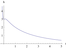
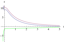
Figure 1: (left) Plot of the Hubble parameter representing the cosmological evolution. The evolution starts from a Big Bang-type singularity and goes through a transient phase of superaccelerated expansion (“phantom era”), which lies between two crossings of PDL (when the derivative of $h$ crosses zero). Then the universe expands infinitely. (right) Plots of the total energy density (blue), and of the energy density of the normal field (purple) and of the phantom one (green).

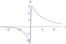
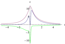
Figure 2: (left) The evolution starts with a contraction in the infinitely remote past. At the point first PDL crossing the contraction becomes superdecelerated and turns in a superaccelerated expansion when $h$ crosses zero. The second PDL crossing ends the “phantom era”; the decelerated expansion continues till the universe begins contracting. In a finite time a Big Crunch-type singularity is reached. (right) Plots of the total energy density (blue), and of the energy density of the normal field (purple) and of the phantom one (green).

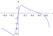
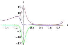
Figure 3: (left) The cosmological evolution begins with a contraction in the infinitely remote past. with the first PDL crossing the contraction becomes superdecelerated until the universe stops ($h=0$) and starts expanding. With the second crossing the “phantom era” ends and the expansion continues infinitely. (right) Plots of the total energy density (blue), and of the energy density of the normal field (purple) and of the phantom one (green).

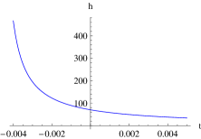
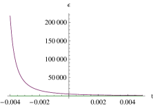
Figure 4: (left) Evolution from a Big Bang-type singularity to an infinite expansion, without any crossing of PDL. This evolution is thus guided by the “normal” field $\phi$. (right) Plots of the total energy density (blue), and of the energy density of the normal field (purple) and of the phantom one (green). Notice that the energy density of the phantom field (green) is very close to zero, thus the total energy density is mainly due to the standard field.

4.1 The cosmological dynamics in the presence of dust like matter

Trying to make our model more realistic we can try to describe which changes does it undergo in the presence of some matter. The natural candidate for the role of matter is a dust-like perfect fluid with the vanishing pressure. In this case the Friedmann equation (13) acquires the form

$$h^{2}=\frac{\dot{\phi}^{2}}{2}-\frac{\dot{\xi}^{2}}{2}+Ae^{\alpha\phi}-Be^{-\beta\xi}+\frac{C_{0}}{a^{3}},$$ (27)

while the second Friedmann equation (22) becomes

$$\dot{h}=-\frac{3}{2}\left(\dot{\phi}^{2}-\dot{\xi}^{2}+\frac{C_{0}}{a^{3}}\right),$$ (28)

where the constant $C_{0}$ characterizes the quantity of the dust-like matter in a universe under consideration.

Obviously at the early stage of the cosmological evolution, this dust contribution into the Friedmann equations dominates over dark energy contribution coming from our scalar fields. So, at early stage of the evolution (close to the Big Bang epoch) the effects like phantomization of the matter content of the universe and phantom divide line crossing are impossible. They are postponed until the time when the expansion of the universe is so large that this additional term becomes insignificant. However, one can say that its presence even underlines some peculiar effects of the considered model. Indeed, it makes stronger the non-phantom part of the matter content of the universe and hence return to the normal non-phantom case occurs more quickly. Naturally, the Big Rip singularity is avoided in this model.

5 Conclusion

As was already said above the data are compatible with the presence of the phantom energy, which, in turn, can be in a most natural way realized by the phantom scalar field with a negative kinetic term. However, such a field suffers from the instability problem, which makes it vulnerable. Inspired by the development of PT symmetric quantum theory[14] we introduced the PT symmetric two-field cosmological model where both the kinetic terms are positive, but the potential of one of the fields is complex. We studied a classical background solution of two Klein-Gordon equations together with the Friedmann equation, when one of this fields (normal) is real while the other is purely imaginary. The scale factor in this case is real and positive just like the energy density and the pressure. The background dynamics of the universe is determined by two effective fields - one normal and one phantom, while the Lagrangian of the linear perturbations has the correct sign of the mass term. Thus, so to speak, the quantum normal theory is compatible with the classical phantom dynamics and the problem of instability is absent.

As a byproduct of the structure of the model, at variance with quintom models, the phantom dominance era is transient, the number of the phantom divide line crossings is even and the Big Rip singularity is excluded. In all our numerical simulations we have seen only two phantom divide line crossings. However, one cannot exclude that at some special initial conditions, or, in the models of the kind considered in the present paper, but with more complicated potentials, it is possible to see more than two phantom divide line crossings. It would be especially interesting to find the potentials or/and initial conditions providing an oscillatorial behaviour with infinite phantom divide line crossings.

References

- [1] C. M. Bender and S. Boettcher, Phys. Rev. Lett. 80 (1998) 5243; C. M. Bender, S. Boettcher and P. Meisinger, J. Math. Phys. 40 (1999) 2201; C. M. Bender, D. C. Brody and H. F. Jones, eConf C0306234 2003 617 [Phys. Rev. Lett. 89, (2002 ERRAT,92,119902.2004) 270401]; C. M. Bender, J. Brod, A. Refig, M. Reuter, J. Phys. A 37 (2004) 10139; C. M. Bender, J. H. Chen and K. A. Milton, J. Phys. A 39 (2006) 1657; C. M. Bender, D. C. Brody, J. H. Chen, H. F. Jones, K. A. Milton and M. C. Ogilvie, Phys. Rev. D 74 (2006) 025016.
- [2] Z. Ahmed, C. M. Bender and M. V. Berry, J. Phys. A 38 (2005) L627;
- [3] A. A. Andrianov, F. Cannata and A. Y. Kamenshchik, J. Phys. A 39 (2006)9975; A. A. Andrianov, F. Cannata and A. Y. Kamenshchik, Int. J. Mod. Phys. D 15 (2006) 1299.
- [4] A. G. Riess et al. [Supernova Search Team Collaboration], Astron. J. 116 (1998) 1009; S. Perlmutter et al. [Supernova Cosmology Project Collaboration], Astrophys. J. 517 (1999) 565.
- [5] V. Sahni and A. A. Starobinsky, Int. J. Mod. Phys. D 9 (2000) 373; V. Sahni and A. A. Starobinsky, Int. J. Mod. Phys. D 15 (2006) 2105. T. Padmanabhan, Phys. Rept. 380 (2003) 235; P. J. E. Peebles and B. Ratra, Rev. Mod. Phys. 75 (2003) 559; E. J. Copeland, M. Sami and S. Tsujikawa, Int. J. Mod. Phys. D 15 (2006) 1753.
- [6] R. R. Caldwell, Phys. Lett. B 545 (2002) 23.
- [7] A. A. Starobinsky, Grav. Cosmol. 6 (2000) 157; R. R. Caldwell, M. Kamionkowski and N. N. Weinberg, Phys. Rev. Lett. 91 (2003) 071301.
- [8] U. Alam, V. Sahni, T. D. Saini and A. A. Starobinsky, Mon. Not. Roy. Astron. Soc. 354 (2004) 275.
- [9] S. M. Carroll, M. Hoffman and M. Trodden, Phys. Rev. D 68 (2003) 023509; S. Sergienko and V. Rubakov, arXiv:0803.3163 [hep-th].
- [10] J. M. Cline, S. Jeon and G. D. Moore, Phys. Rev. D 70 (2004) 043543.
- [11] A. A. Andrianov, Ann. Phys. 140 (1982) 82; A. A. Andrianov, Phys. Rev. D 76 (2007) 025003.
- [12] F. G. Scholtz, H. B. Geyer and F. J. H. Hahne, Ann. Phys. 213 (1992) 74; P. Dorey, C. Dunning and R. Tateo, J. Phys. A 34 (2001) L391.
- [13] F. Cannata, G. Junker and J. Trost, Phys. Lett. A 246 (1998) 219; T. Curtright and L. Mezincescu, J. Math. Phys. 48 (2007) 092106.
- [14] C. M. Bender, Rept. Prog. Phys. 70 (2007) 947.
- [15] A. Mostafazadeh, arXiv:0810.5643 [quant-ph].
- [16] G. ’t Hooft and S. Nobbenhuis, Class. Quant. Grav. 23 (2006) 3819. R. Erdem, Phys. Lett. B 639 (2006) 348; A. A. Andrianov, F. Cannata, P. Giacconi, A. Y. Kamenshchik and R. Soldati, Phys. Lett. B 651 (2007) 306.
- [17] X. L. Feng, X. L. Wang and X. M. Zhang, Phys. Lett. B 607 (2005) 35; L. Perivolaropoulos, Phys. Rev. D 71 (2005) 063503; G. B. Zhao, J. Q. Xia, M. Li, B. Feng and X. Zhang, Phys. Rev. D 72 123515 (2005); J. Q. Xia, B. Feng and X. M. Zhang, Mod. Phys. Lett. A 20 2409 (2005); B. Feng, M. Li, Y. S. Piao and X. Zhang, Phys. Lett. B 634 101 (2006); Z. K. Guo, Y. S. Piao, X. M. Zhang and Y. Z. Zhang, Phys. Lett. B 608 177 (2005); H. Wei, R. G. Cai and D. F. Zeng, Class. Quant. Grav. 22 3189 (2005); R. Lazkoz and G. Leon, Phys. Lett. B 638 303 (2006); X. F. Zhang and T. Qiu, Phys. Lett. B 642 187 (2006); W. Zhao, Phys. Rev. D 73 123509 (2006); M. Alimohammadi and H. M. Sadjadi, Phys. Lett. B 648 113 (2007); Z. K. Guo, Y. S. Piao, X. Zhang and Y. Z. Zhang, Phys. Rev. D 74 127304 (2006); Y. f. Cai, H. Li, Y. S. Piao and X. m. Zhang, Phys. Lett. B 646 141 (2007); X. Zhang, Phys. Rev. D 74 103505 (2006); M. R. Setare, Phys. Lett. B 641 130 (2006); Y. f. Cai, M. z. Li, J. X. Lu, Y. S. Piao, T. t. Qiu and X. m. Zhang, Phys. Lett. B 651 1 (2007); R. Lazkoz, G. Leon and I. Quiros, Phys. Lett. B 649 103 (2007); M. Alimohammadi, Gen. Rel. Grav. 40 107 (2008); M. R. Setare and E. N. Saridakis, Phys. Lett. B 668 177 (2008); J. Sadeghi, M. R. Setare, A. Banijamali and F. Milani, Phys. Lett. B 662 92 (2008); H. H. Xiong, Y. F. Cai, T. Qiu, Y. S. Piao and X. Zhang, Phys. Lett. B 666 212 (2008); Y. F. Cai and J. Wang, Class. Quant. Grav. 25 165014 (2008); S. Zhang and B. Chen, Phys. Lett. B 669 4 (2008); M. R. Setare and E. N. Saridakis, Int. J. Mod. Phys. D 18 549 (2009); M. R. Setare and E. N. Saridakis, JCAP 0809 026 (2008); M. R. Setare and E. N. Saridakis, Phys. Lett. B 671 331 (2009); K. Nozari, M. R. Setare, T. Azizi and N. Behrouz, Phys. Scripta 80 025901 (2009); M. R. Setare and E. N. Saridakis, Phys. Rev. D 79 043005 (2009); L. P. Chimento, M. Forte, R. Lazkoz and M. G. Richarte, Phys. Rev. D 79 043502 (2009); E. N. Saridakis, arXiv:0903.3840 [astro-ph.CO]; H. Wei and S. N. Zhang, Phys. Rev. D 76 063005 (2007); Y. F. Cai, E. N. Saridakis, M. R. Setare and J. Q. Xia, arXiv:0909.2776 [hep-th]; H. Zhang, arXiv:0909.3013 [astro-ph.CO].
- [18] V. Buslaev and V. Grecchi, J. Phys. A 26 (1993) 5541.
- [19] F. Lucchin and S. Matarrese, Phys. Rev. D 32 (1985) 1316; J. J. Halliwell, Phys. Lett. B 185 (1987) 341. A. B. Burd and J. D. Barrow, Nucl. Phys. B 308 (1988) 929; V. Gorini, A. Y. Kamenshchik, U. Moschella and V. Pasquier, Phys. Rev. D 69 (2004) 123512.
- [20] A. A. Andrianov, F. Cannata and A. Y. Kamenshchik, Phys. Rev. D 72 (2005) 043531.
- [21] F. Cannata and A. Y. Kamenshchik, Int. J. Mod. Phys. D 16 (2007) 1683;
- [22] R. Gannouji, D. Polarski, A. Ranquet and A. A. Starobinsky, JCAP 0609 (2006) 016.
- [23] P. Callin and F. Ravndal, Phys. Rev. D 72 (2005) 064026.
- [24] A. A. Andrianov and L. Vecchi, Phys. Rev. D 77 (2008) 044035.