Parametrization and Classification of 20 Billion LSST Objects: Lessons from SDSS

Abstract

The Large Synoptic Survey Telescope (LSST) will be a large, wide-field ground-based system designed to obtain, starting in 2015, multiple images of the sky that is visible from Cerro Pachon in Northern Chile. About 90% of the observing time will be devoted to a deep-wide-fast survey mode which will observe a 20,000 deg² region about 1000 times during the anticipated 10 years of operations (distributed over six bands, $ugrizy$). Each 30-second long visit will deliver 5$\sigma$ depth for point sources of $r\sim 24.5$ on average. The co-added map will be about 3 magnitudes deeper, and will include 10 billion galaxies and a similar number of stars. We discuss various measurements that will be automatically performed for these 20 billion sources, and how they can be used for classification and determination of source physical and other properties. We provide a few classification examples based on SDSS data, such as color classification of stars, color-spatial proximity search for wide-angle binary stars, orbital-color classification of asteroid families, and the recognition of main Galaxy components based on the distribution of stars in the position-metallicity-kinematics space. Guided by these examples, we anticipate that two grand classification challenges for LSST will be 1) rapid and robust classification of sources detected in difference images, and 2) simultaneous treatment of diverse astrometric and photometric time series measurements for an unprecedentedly large number of objects.

1 Parametrization of LSST Objects

Instead of discussing numerous classification techniques that are the main topic of this conference, we focus on the properties of measured parameters that represent input to various classification algorithms and methods. We summarize the anticipated measurements for LSST, and provide a few classification examples based on similar SDSS data.

1.1 A brief overview of LSST

The Large Synoptic Survey Telescope (LSST) will be a large, wide-field ground-based system designed to obtain multiple images covering the sky that is visible from Cerro Pachon in Northern Chile. The system design is driven by four main science themes: probing dark energy and dark matter, taking an inventory of the Solar System, exploring the transient optical sky, and mapping the Milky Way. For a detailed discussion of LSST science drivers, baseline design, and anticipated data products, please see Ivezić et al. (2007a).

Briefly, the current baseline design, with an 8.4m (6.5m effective) primary mirror, a 9.6 sq.deg. field of view, and a 3.2 Gigapixel camera, will allow about 10,000 deg² of sky to be covered each night (using pairs of 15-second exposures), with an average revisit time of three nights and 5-sigma depth for point sources of $r\sim 24.5$. The survey area will include 30,000 deg² with $\delta<34.5^{\circ}$, and will be imaged multiple times in six bands, $ugrizy$, covering the wavelength range 320–1050 nm. About 90% of the observing time will be devoted to a deep-wide-fast survey mode which will observe, starting in 2015, a 20,000 deg² region about 1000 times during the anticipated 10 years of operations (including all six bands). These data will result in databases including 10 billion galaxies and a similar number of stars, and will serve the majority of science programs.

1.2 The measured parameters for LSST Sources and Objects

The rapid cadence of the LSST observing will produce an enormous volume of data, $\sim$30 TB per night, leading to a total database over the ten years of operations of 60 PB for the compressed raw data, and 30 PB for the catalog database. The total data volume after processing will be several hundred PB, processed using $\sim$100 TFlops of computing power. Processing such a large volume of data, converting the raw images into a faithful representation of the Universe, automated data quality assessment, and archiving the results in useful form for a broad community of users is a major challenge.

The two main data deliverables will be transient event reporting, and yearly data releases. The transient event reporting system will send out alerts to the community within 60 seconds of completing the image readout. Yearly data releases are intended to produce the most completely analyzed data products of the survey (in particular those that measure very faint objects and cover long time scales). The transient event reporting system will be based on difference image analysis and will include classification based on measured properties in the event image, as well as on properties of the local background determined from template images (see Bailey et al. 2007, Becker 2008, and Borne 2008 for examples of ongoing work). We limit discussion here to recurrent sources (as opposed to one-time events such as various explosions).

For each of $\sim$20 billion objects detected in deep images, the time series of positions, $\alpha(t)$ and $\delta(t)$, and magnitudes, $m(t);m=(u,g,r,i,z,y)$, will be measured (detections in individual images are called “sources”, and they are associated into “objects”). The systematic errors in positions will be of the order 10 mas, and photometric errors will be about 5 millimag at the bright end. While automated pipelines will measure several types of magnitudes (e.g. point spread function, model, Petrosian, etc.), as well as higher image moments, such as image shape and size, for simplicity here we only consider the above listed generic quantities (however, for a spectacular example of an astronomical source with time-varying morphology see Rest et al. 2005). Morphological information will be used for star-galaxy separation. We ignore this important classification problem in this paper. Of course, morphological information will be used to separate comets from asteroids as well, to classify galaxies (e.g. via bulge-disk decomposition), and the measurements of galaxy shapes will form the basis of weak lensing studies.

Given the above three time series, $\alpha(t),\delta(t)$, and $m(t)$, sampled about 1000 times over 10 years, for a sample of 20 billion objects, it is not obvious how to perform efficient and robust classification. Even if the measurement errors are ignored, there are about 60 trillion numerical values to analyze! Alternatively, one needs to quantitatively describe a 3000-dimensional space populated by 20 billion points. The current practice and experience is such that one would not blindly feed this dataset to a computer algorithm and hope for an ultimate and complete classification. Rather, both the choice of measurements and applied computational techniques would be driven by specific science goals. For example,

1. For slow moving objects such as stars (motion is typically smaller than arcsec per year), $\alpha(t)$ and $\delta(t)$ are modeled as a superposition of linear motion due to star’s space velocity, the reflex motion due to Earth’s revolution (trigonometric parallax), and possibly of the orbital motion in a multiple star system. Displacements between two successive observations are much smaller than the seeing disk, and thus there is practically no ambiguity when associating different detections. This modeling yields trigonometric parallax, proper motion vector, and orbital properties.

2. For fast moving objects such as asteroids and other solar system objects (motion is typically larger than arcmin per year, and for nearby asteroids faster than degree per day), displacements between two successive observations are much larger than the seeing disk, and often can be larger than the typical distance between two (stationary) objects. Thus, associations of different detections may be highly uncertain, and to resolve the ambiguity $\alpha(t)$ and $\delta(t)$ are required to be consistent with a nearly-Keplerian orbital motion. This analysis yields six orbital parameters for each object.

3. The time-averaged values of $m(t)$ enable the construction of color-magnitude and color-color diagrams. These diagrams can be used to classify objects, as well as to derive additional, typically more physically relevant, parameters, such as photometric redshift for galaxies and quasars, photometric distance, effective temperature and metallicity for stars, and taxonomy for asteroids.

4. Detailed properties of light curves, $m(t)$, such as shape, amplitude and period for periodic variables, or the structure function for aperiodic variability, often enable powerful classification schemes (e.g. the classification of variable stars in the amplitude-period diagram). The current LSST plans call for automatic computation of numerous parameters that are designed to capture detailed statistical properties of light curves (e.g. low-order moments, period, amplitude).

5. Measurements for individual objects need not be analyzed in isolation; rather, they can be considered in relation to measurements of neighboring objects.

We proceed to provide concrete examples of each type of classification based on SDSS data.

2 Examples of Classification

In many aspects, SDSS data are similar to anticipated LSST data. In particular, the photometric systems are similar, and SDSS provides some time domain data (light curves, proper motion, solar system objects). LSST will extend the coverage down to 60 sec timescale, and to much fainter objects. Thus, the ongoing classification work based on SDSS data can serve as a preview of what will be possible to do with LSST on a much larger scale.

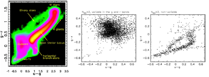
Figure 1: The left panel shows the $g-r$ vs. $u-g$ color-color diagram for two million stars measured by SDSS (adapted from Smolčić et al. 2004). Accurate $ugr$ photometry enables detailed and robust classification. The middle and right panel show the zoomed-in lower-left corner of this diagram (adapted from Ivezić et al. 2007b), with sources classified by their photometric variability into highly variable (middle; dominated by quasars) and non-variable (right; dominated by H and He white dwarfs). LSST will obtain such measurements and enable resulting classification for billions of stars and millions of quasars.

2.1 Classification based on colors

The position of a source in the $g-r$ vs. $u-g$ color-color diagram (Fig. 1) contains rich information that can be used for preliminary source classification. Determination of detailed stellar properties such as effective temperature and metallicity can further improve the resulting classification (see left panel in Fig. 2), as well as the addition of data from more bandpasses.

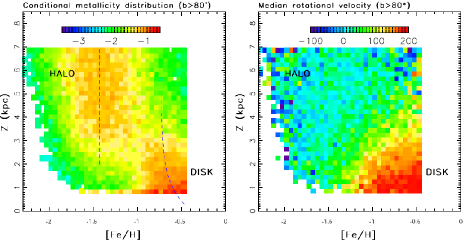
Figure 2: An illustration of stellar classification based on $ugr$ photometry and proper motion measurement. The left panel shows the photometric metallicity distribution, as a function of the distance from the Galactic plane, for about 60,000 F/G main-sequence stars within 10 degrees from the North Galactic Pole (adapted from Ivezić et al. 2008). The distribution is displayed on a logarithmic scale and color-coded as shown in the inset. Two distinct Galaxy components, halo and disk, are marked. The dashed lines mark the median metallicity for each component. These two components with distinct metallicity distributions also have different kinematics, as illustrated in the right panel. The color-coded map shows the median rotational velocity component for the same stars as in the left panel. The velocity is determined from displacements of stars on the sky over half a century that lapsed between the Palomar Observatory Sky Survey in the 1950s and SDSS. The high-metallicity disk stars have large rotational velocity (about 200 km/s, see the inset), while the low-metallicity halo stars display behavior consistent with no net rotation.

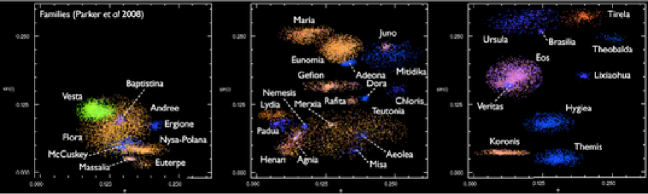
Figure 3: An illustration of classification based on photometry and orbital motion parameters. The three panels show the distribution of main-belt asteroids in the orbital inclination vs. eccentricity space, for three regions selected by the orbital semi-major axis (adapted from Parker et al. 2008). Each dot represents one asteroid, and is color-coded according to its colors measured by SDSS. The families are defined by simultaneously applying Gaussian filters in orbital and color space.

2.2 Classification based on motion

The moving objects naturally split into two classes: slow stellar motion and fast motion of solar system objects. Fig. 2 illustrates how proper motion measurements can be used to classify stars into disk and halo populations. This can be applied to other types of objects. The simultaneous use of orbital parameters and color to associate asteroids into families (remnants of larger bodies destroyed in collisions) is illustrated in Fig 3.

2.3 Classification based on photometric variability

The color information can be augmented with variability information to further improve source classification. For example, the right panel in Fig. 1 shows that the $u-g$ color distribution of non-variable sources with blue $g-r$ colors is tri-modal – evidently, the information content is very high! The bluest branch is consistent with He white dwarfs, the middle branch with hydrogen white dwarfs, and the reddest branch is made of blue horizontal branch stars (see Ivezić et al. 2007b for more details and references).

The statistical properties of light curves have long been used for robust classification, especially when multi-color data are available. Fig. 4 illustrates classification of RR Lyrae stars with the aid of multi-color light curves. It is estimated that LSST will detect and parametrize about 100 million variable stars.

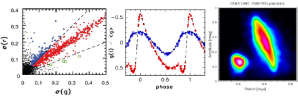
Figure 4: An illustration of classification based on colors and light curve shape, period and amplitude. The left panel shows a relationship between the photometric root-mean-square scatter measured in SDSS $g$ and $r$ bands for point sources with colors typical of RR Lyrae stars (marked by “horizontal branch stars” in Fig. 1). The two dashed lines mark the region consistent with RR Lyrae light curves (for details see Sesar et al. 2007). The middle panel shows examples of RR Lyrae light curves (blue: c type, red: ab type) measured by SDSS. The right panel shows the distribution of RR Lyrae stars of both types in the amplitude vs. period diagram (measured by the OGLE survey; adapted from Eyer & Mowlavi 2007).

2.4 Classification involving neighbors

In addition to measurements for an individual object, measurements of its neighboring objects (either in spatial proximity, or using an arbitrary parameter) can be used in classification. For example, Sesar et al. (2008) developed a method for selecting candidate wide-angle stellar binary systems by requiring i) spatial proximity of two stars on the sky, ii) similarity of their photometric distances, and iii) similarity of their proper motion vectors (Fig. 5). Strong gravitational lensing of supernovae is another example.

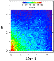
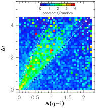
Figure 5: An illustration of the simultaneous use of photometry and astrometric proximity to nearby sources to select pairs of stars that are good candidates for wide-angle binary systems (adapted from Sesar et al. 2008). The left panel shows the distribution of stellar pairs from a random SDSS sample in the magnitude difference vs. color difference diagram. The middle panel shows analogous diagram for stellar pairs with component separation in the range 3–4 arcsec. This sample shows an excess of pairs whose magnitude and color differences are consistent with the same distance from us (via photometric parallax relation), as demonstrated by the ratio of the two maps shown in the right panel.

3 Discussion

The classification challenge for recurrent LSST sources can be phrased as: given three time series, $\alpha(t),\delta(t)$, $m(t)$, and associated morphology, sampled 1000 times over 10 years, for 20 billion objects, assign objects to known populations, discover new populations, and quantify their behavior. The current practice and experience argue that there is no “one size fits all” solution; rather, the choice of measurements and applied computational techniques is driven by specific science goals, as briefly illustrated by examples presented here. The requirements for rapid and robust classification of transient sources present additional challenges. We invite experts in the fields of parametrization and classification to join LSST effort and contribute timely solutions to these challenges.

References

- (1) Bailey, S., Aragon, C., Romano, R., et al. 2007, ApJ, 665, 1246
- (2) Becker, A.C. 2008, Astronomische Nachrichten, 329, 280
- (3) Borne, K.D. 2008, Astronomische Nachrichten, 329, 255
- (4) Eyer, L. & Mowlavi, N. 2007, astro-ph/0712.3797
- (5) Ivezić, Ž., Tyson, J.A., Allsman, R., et al. 2007a, astro-ph/0805.2366
- (6) Ivezić, Ž., Smith, J. A., Miknaitis, G., et al. 2007b, AJ, 134, 973
- (7) Ivezić, Ž., Sesar, B., Jurić, M., et al. 2008, ApJ, 684, 287
- (8) Parker, A., Ivezić, Ž. & Jurić, et al. 2008, Icarus, in press (astro-ph/0807.3762)
- (9) Rest, A., Suntzeff, N.B., Olsen, K., et al. 2005, Nature, 438, 1132
- (10) Sesar, B., Ivezić, Ž., Lupton, R.H., et al. 2007, AJ, 134, 2236
- (11) Sesar, B., Ivezić, Ž. & Jurić, M. 2008, ApJ, in press (astro-ph/0808.2282)
- (12) Smolčić, V., Ivezić, Ž., Knapp, G.R., et al. 2004, ApJ, 615, L141