Time Variability of Quasars: the Structure Function Variance

Abstract

Significant progress in the description of quasar variability has been recently made by employing SDSS and POSS data. Common to most studies is a fundamental assumption that photometric observations at two epochs for a large number of quasars will reveal the same statistical properties as well-sampled light curves for individual objects. We critically test this assumption using light curves for a sample of $\sim$2,600 spectroscopically confirmed quasars observed about 50 times on average over 8 years by the SDSS stripe 82 survey. We find that the dependence of the mean structure function computed for individual quasars on luminosity, rest-frame wavelength and time is qualitatively and quantitatively similar to the behavior of the structure function derived from two-epoch observations of a much larger sample. We also reproduce the result that the variability properties of radio and X-ray selected subsamples are different. However, the scatter of the variability structure function for fixed values of luminosity, rest-frame wavelength and time is similar to the scatter induced by the variance of these quantities in the analyzed sample. Hence, our results suggest that, although the statistical properties of quasar variability inferred using two-epoch data capture some underlying physics, there is significant additional information that can be extracted from well-sampled light curves for individual objects.

1 Introduction

Significant progress in the description of quasar variability has been recently made by employing SDSS data. Vanden Berk et al. (VB2004 , hereafter VB) compared imaging and spectrophotometric magnitudes to investigate the correlations of variability with rest-frame time lag (up to 2 years), luminosity, rest-frame wavelength, redshift, the presence of radio and X-ray emission, and the presence of broad absorption line outflows. Variability on longer time scales was studied by de Vries, Becker, White, and Loomis (dV2005 , hereafter dVBWL; Sesar2006 ) who compared SDSS and POSS photometric measurements. Ivezić et al. (ive2004 , hereafter, I04) used repeated SDSS imaging scans, which increased the measurement accuracy for magnitude differences by about a factor of 3-4 compared to studies based on spectrophotometric magnitudes, and also enabled analysis of the $u$ and $z$ band variability.

Common to these and similar studies is a fundamental assumption that photometric observations at two epochs for a large number of quasars will reveal the same statistical properties as well-sampled light curves for individual objects. We critically test this assumption using light curves for a sample of $\sim$2,600 spectroscopically confirmed quasars observed by the multi-epoch SDSS stripe 82 survey. We describe these observations and our methodology in the next section, and analyze the data in Section 3.

2 SDSS Stripe 82 Data and Methodology

We study a sample of about 2,600 spectroscopically confirmed quasars (see Sch2007 for the SDSS Quasar Catalog) imaged about 50 times on the average over 8 years (for details see Sesar2007 ). These data were obtained in yearly “seasons” about 2-3 months long. We average observations within each season, and construct a structure function (see dVBWL for definition) for each object for an observed time lag of 1 year, and in each of the five SDSS bandpasses ($ugriz$). The total number of structure function data points for all quasars and bands is 10,370. We correct for cosmological time dilation and length contraction and obtain a fairly well-sampled plane of the rest-frame quantities $\Delta t_{RF}$ and $\lambda_{RF}$ (spanning from about 100 to 300 days and 1000 to 6000 Å).

To compare the statistical properties of quasar variability inferred from two-epoch data, and those based on light curves for individual objects, we use a quasar variability model from I04. Using $\sim$66,000 magnitude difference measurements, $\Delta m$, for a sample of $\sim$13,000 quasars, they found that $\Delta m$ follow an exponential distribution, $p(\Delta m)\propto exp(-|\Delta m|/\Delta_{c})$, where the characteristic variability scale, $\Delta_{c}$ is a function of rest-frame time lag ($\Delta t_{RF}$, days), wavelength ($\lambda_{RF}$, Å), and absolute magnitude in the $i$ band ($M_{i}$) (the variability scale is related to the more commonly used structure function by $SF=\sqrt{2}\Delta_{c}$). Their simple model for the variability scale,

$$SF=(1.00\pm 0.03)[1+(0.024\pm 0.04)\,M_{i}]\left(\frac{\Delta t_{RF}}{\lambda_{RF}}\right)^{0.30\pm 0.05}$$ (1)

describes $\Delta m$ measurements to within the measurement noise ($\sim$0.02 mag). Note that there is no dependence on redshift (see Fig. 1).

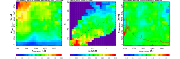
Figure 1: (Figure 1 from I04) The left panel displays the measured structure function as a function of rest-frame time lag and wavelength (each pixel contains $\sim 25$ objects). The middle panel shows the structure function in a narrow range of rest-frame time lag and wavelength (100 days$<\Delta t_{RF}<$150 days, 1000Å$<\lambda_{RF}<$2000 Å), as a function of redshift and luminosity. The lines of constant variability are nearly parallel to the redshift axis, suggesting that the dependence of variability on luminosity is much stronger than the dependence on redshift. The right panel displays the difference between the data shown in the left panel and the best-fit model described by Eq. (1). The over-plotted line shows the composite quasar spectrum from VB2001 . The negative residuals at $\sim$2800 Å are due to the anti-correlation of continuum and MgII line variability.

We attempted to fit the same functional form to the SF data obtained for individual objects from stripe 82. We find that the observed SF is still well-fit using a single exponent for $\lambda_{RF}$ and $\Delta t_{RF}$, except with a value for the exponent of $0.47\pm 0.02$. The parameters used to model the observed SF are measured in the ranges 1000Å ¡ $\lambda_{RF}$¡ 6000Å, 100 days $<\Delta t_{RF}<300$ days (compared to 0-600 days for the two-epoch sample), and $-29<M_{i}<-23$. This modified model SF provides a good description of the observed SF; the ratio of the observed to model SF does not show any systematic behavior with respect to $\Delta t_{RF}$, $\lambda_{RF}$, $M_{i}$, or redshift.

The similarity of the mean structure function computed for individual quasars and the structure function derived from the two-epoch observations of a much larger sample suggests that the statistical properties of quasar variability inferred using only two epochs for a large number of quasars are representative of the underlying physics. This is at least true for the overlap in their timescales (i.e., for timescales $\sim$300 days or less). We proceed with analysis of the distribution of the ratio of observed ($SF_{obs}$) and modeled ($SF_{model}$) structure functions.

3 Analysis: the Structure Function Variance

The distribution of $SF_{obs}/SF_{model}$ values for the two-epoch sample analyzed by I04 is shown in the upper left panel in Fig. 2. It is well described by a Gaussian distribution with $\sigma=0.09$. That is, the model describes the mean behavior of SF as a function of luminosity, rest-frame wavelength and time to within $\sim$10% of the measured values. However, the analysis based on two-epoch data cannot provide information about SF variance in a bin with fixed values of $M_{i}$, $\Delta t_{RF}$, and $\lambda_{RF}$. This is because the SF is constructed using the magnitude difference measurements from all the quasars. Their scatter measures the mean value of the SF, but provides no information about the SF variance among individual objects. To measure the latter, individual light curves must be available.

The distribution of $SF_{obs}/SF_{model}$ values for the sample analyzed here, where SF is evaluated for every individual object from its light curve, is also shown in the upper left panel in Fig. 2. It is much wider than the corresponding distribution based on two-epoch sample (which covers a larger range in $\Delta t_{RF}$), clearly non-Gaussian, and well-fit by a sum of two Gaussians. In fact, the scatter in $SF_{obs}/SF_{model}$ for fixed values of $M_{i}$, $\Delta t_{RF}$, and $\lambda_{RF}$, is similar to the scatter induced by the variance of these quantities. The published analysis, exemplified by VB, dVBWL and I04 work, captured the mean trends, but not the surprisingly large scatter around the mean behavior ($\sigma\sim 0.4$). This new result demonstrates that there is significant additional information that can be extracted from well-sampled light curves for individual objects.

At this stage of analysis it is not clear what causes the SF scatter. One obvious candidate is intrinsic stochasticity of the process causing variability (e.g. see discussion in Kawa1998 ). We are also revisiting issues such as photometric calibration of SDSS stripe 82 data and the robustness of SF analysis to non-Gaussian outliers (the distribution of two-epoch magnitude differences follows an exponential, rather than Gaussian, distribution; I04). It will also be helpful in the future to repeat this analysis for better-sampled light curves.

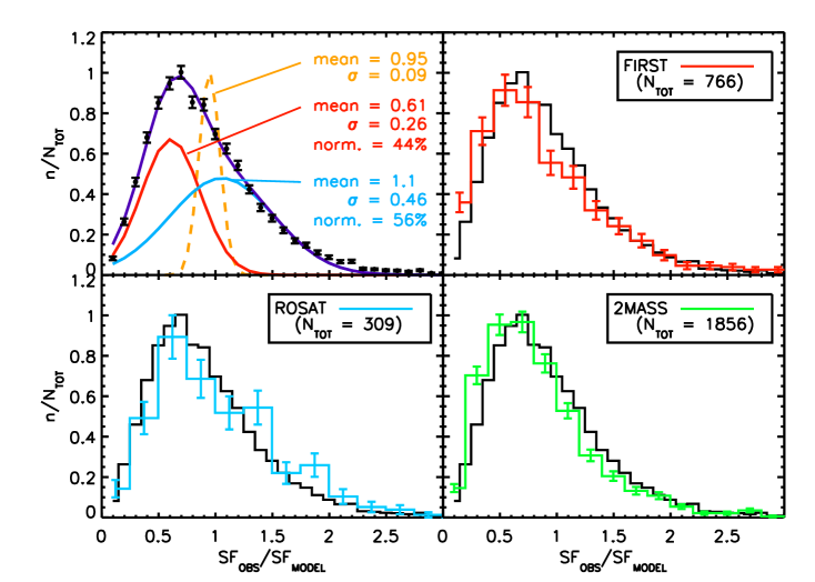
Figure 2: Distribution of $SF_{obs}/SF_{model}$. The distribution from analysis by I04 based on two-epoch data is shown by the dashed curve (scaled by a factor of 0.2). The symbols with error bars show the distribution obtained here, that is based on SF measured for each individual object ($n$ is defined as the number of points in a bin ($N_{bin}$) divided by the bin width ($\Delta_{bin}$), and $N_{TOT}$ is the total number of points used for each histogram; that is, the enclosed area is unity). Error bars are computed as $\sqrt{N_{bin}}/(N_{TOT}\Delta_{bin})$. The curve passing through the data points is an empirical fit that is the sum of the two solid (Gaussian) curves below it, with relative normalizations of 44% and 56%. The same total distribution is shown as the dark histogram in the other three panels, where it is compared to analogous distributions for radio (top-right), X-ray (lower-left), and infrared (lower-right) subsamples.

3.1 The SF for Subsamples with Detections at Other Wavelengths

We investigated whether the distribution of $SF_{obs}/SF_{model}$ for the sample analyzed here varies among various subsamples. First we compared the distribution for the whole sample to the distribution obtained for the apparently brightest 10% objects in the $i$ band, and did not detect any statistically significant difference. We also created subsamples that are detected in 2MASS, FIRST, and ROSAT, as listed in Sch2007 . Out of the 10,370 total data points, 1856 (or $\sim$400 quasars) have infrared ($J$, $H$, and $K$) detections, 766 ($\sim$150 quasars) have radio detections, and 309 ($\sim$70 quasars) have X-ray detections.

The distribution of $SF_{obs}/SF_{model}$ for each of these subsamples is compared to that of the entire sample in Fig. 2. While the ROSAT sample seems to follow the distribution for the whole sample, the FIRST and 2MASS samples appear skewed toward lower values of $SF_{obs}/SF_{model}$, indicating less variability compared to the optically selected sample. We also investigated the behavior of $SF_{obs}/SF_{model}$ values as a function of optical and infrared colors $i-K$ and $J-K$, optical-radio “color” $i-t$, and X-ray-optical “color” $x-i$ ($t$ and $x$ are radio and X-ray AB magnitudes, see ive2002 ). Figure 3 shows that the quantity $SF_{obs}/SF_{model}$ is independent of $i-K$ and $J-K$ colors. However, there seems to be a positive correlation with $i-t$: optical variability increases with radio loudness, in agreement with VB, who found that radio-bright quasars are about 1.3 times more variable. There is no significant correlation with $x-i$ color.

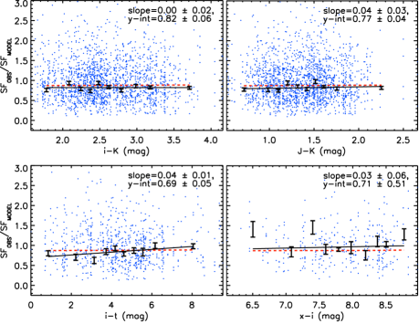
Figure 3: The ratio of observed SF to model SF is plotted against $i-K$, $J-K$, $i-t$, and $x-i$ colors as dots. These data points are then divided into bins of $N$ points, where $N$ is set to 10% of the total number of points. The median values for each bin along with $1\sigma$ error bars are shown, where $\sigma=0.926$(interquartile range)$/\sqrt{N-1}$. The over-plotted solid lines are linear regressions for the median values (the fit parameters are listed in the upper-right corners) and the over-plotted dashed lines are the same, but for the entire sample of 10,370 data points.

References

- (1) D. E. Vanden Berk, B. C. Wilhite, R. G. Kron, and 11 co-authors, Astrophys. J., 601, 692 (2004).
- (2) W. H. de Vries, R. H. Becker, R. L. White, and C. Loomis, Astron. J., 129, 615, (2005).
- (3) B. Sesar, D. Svilković, Ž. Ivezić, and 14 co-authors, Astron. J., 131, 2801 (2006).
- (4) Ž. Ivezić, et al., “Quasar Variability Measurements With SDSS Repeated Imaging and POSS Data” in The Interplay Among Black Holes, Stars and ISM in Galactic Nuclei, edited by T. S.-B., L. C. H., and H. R. S., Proceedings of IAU Symposium, No. 222, Cambridge University Press, Cambridge, 2004, pp. 525-526.
- (5) D. P. Schneider et al., Astron. J., 134, 102 (2007).
- (6) B. Sesar et al., Astron. J., 134, 2236 (2007).
- (7) D. E. Vanden Berk, G. T. Richards, A. Bauer, and 59 co-authors, Astron. J., 122, 549 (2001).
- (8) T. Kawaguchi, S. Mineshige, M. Umemura, and E. L. Turner, Astrophys. J., 504, 671 (1998).
- (9) Ž. Ivezić et al., Astron. J., 124, 2364 (2002).