Langevin formulation for single-file diffusion

Abstract

We introduce a stochastic equation for the microscopic motion of a tagged particle in the single file model. This equation provides a compact representation of several of the system’s properties such as Fluctuation-Dissipation and Linear Response relations, achieved by means of a diffusion noise approach. Most important, the proposed Langevin Equation reproduces quantitatively the three temporal regimes and the corresponding time scales: ballistic, diffusive and subdiffusive.

I Introduction

Since its introduction in 1965 due to Harris’ pioneering work Harris , the single file model (SF) has attracted more and more interest among the scientific community. Introduced first in the mathematical physics literature as an interesting though somewhat exotic topic, it has inspired over the last 40 years a large body of profound theoretical studies SF_basic and detailed numerical investigations, including extensive Monte-Carlo and molecular dynamics simulations SF_numerics .

The motivations for the longstanding interest in this topic reside, on one hand, in its analytical tractability and, on the other hand, in its effectiveness as a description of diffusion phenomena in real quasi one dimensional systems. As a matter of fact, since the direct observation and manipulation of nanoscopic systems has exponentially evolved in the last decade, models suitable to account for the single particle diffusional mechanisms in constrained flow geometries, have been subjects of increasing attention. Remarkably, among these, the SF holds a preeminent position, since it correctly reproduces transport properties in a large category of quasi one dimensional systems, where each particle is free to diffuse against its neighbors but is forbidden to overcome them SF_modelz . Transport processes of this type may be observed in nanoporous materials Karger_Book , in collective motion of ions through biological channels and membranes Aidley_Book as well as in nanodevices and cellular flows Albert_Book

Along a mathematical line, the SF is perhaps the simplest interacting one dimensional gas one can consider: it consists of N unit-mass particles constrained to move along a line following a given dynamics. As the particles’ interaction is purely hard-core, no mutual exchanges of the diffusants are allowed, i.e. they retain their ordering over time (single filing condition). In spite of the intricacies of its mathematical derivation, the long time behavior of the single file dispersion relation can be cast in the following suggestive form SF_basic

$$\delta x^{2}(t)=\frac{\langle\left|X\right|\rangle}{\rho}$$ (1)

where $\rho=\frac{N}{L}$ ($N\to\infty$, $L\to\infty$) is the file’s density and $\langle\left|X\right|\rangle$ is the absolute displacement of a non-interacting particle. If the free particle dynamics is characterized by a diffusivity $D=k_{B}T/\gamma$, then the relation (1) takes the form SF_basic2

$$\delta x^{2}(t)=2\sqrt{\frac{D\,t}{\pi\rho^{2}}}.$$ (2)

The predicted subdiffusive behavior has been reproduced experimentally in colloidal particles systems colloidal and observed in molecular sieves (zeolites) zeolites . We remark that the subdiffusive behavior represented by Eq. (2) will eventually be replaced by regular diffusion if for instance the particles are allowed to overtake each other mon , if there is only a finite number of particles kumasl , or the particles move in a ring beijeren .

In Ref.Marchesoni it was pointed out that the subdiffusive regime of a SF tagged particle occurs on the score of long ranged anticorrelations of its velocity, and/or of the jump’s statistics of the collisional mechanism underlying its dynamics. Beside these persistent memory effects, different mathematical derivations agree with the fact that asymptotically the tagged particle’s probability distribution must be Gaussian with a variance growing in time according to (2) SF_basic . Together, these properties contrast with the Continuous Time Random Walk (CTRW) scheme and its corresponding Fokker Planck representation, for which a stretched Gaussian solution has to be expected (see Ref.Klafter and references therein). Furthermore, several subdiffusive systems in nature share the property of Gaussianicity with the SF, e.g. a monomer in a one dimensional phantom polymer phantom_monomer , the “translocation coordinate” of a two dimensional Rouse chain through a hole Kantor , a tagged monomer in an Edward-Wilkinson chain Alberto , de Gennes’ defects along a polymer during its reptation DeGennes and solitons in the sine-Gordon chain solitons .

In this paper we address the question of the microscopic effective description of the stochastic, anomalous motion of the tagged particle. Our aim is to extend the valuable Langevin approach, valid for the case of a diffusive Brownian walker, to the subdiffusive dynamics of a SF particle. We anticipate here that the Generalized Langevin Equation (GLE) Mori ; Kubo provides the ideal theoretical tool for such a goal, incorporating all the statistical properties enjoyed by the particle. Within this framework the non-Markovian memory effects are achieved by means of a power-law damping kernel Lutz , which is simply added algebraically to the instantaneous friction of the surroundings. We note here that the GLE has recently been successfully used to describe several physical phenomena and market flows GLE_articles .

The article is organized as follows: in sec.II we study the density profile dynamics by means of a Diffusion-noise approach and we connect the file’s density fluctuations to the motion of a tagged particle. In sec.III we introduce the GLE and we show the accuracy of the Langevin description by means of extensive molecular dynamic simulations.

II Diffusion noise approach

We start by considering the file density dynamics. As stated in I, the system is composed of $N$ Brownian point-like particles, all of unit mass, moving along a ring of length $L$ and performing a stochastic motion according to the Langevin Equation (LE):

$$\begin{array}[]{l}\dot{x_{i}}(t)=v_{i}(t)\\ \dot{v_{i}}(t)=-\gamma v_{i}(t)+\xi_{i}(t),\end{array}$$ (3)

where $i\in[1,N]$ denotes the particle’s index, and the damping coefficient $\gamma$ and the random noise source $\xi_{i}(t)$ satisfy the well-known Fluctuation-Dissipation Relation (often called second Kubo Theorem Kubo ) $\langle\xi_{i}(t)\rangle\xi_{j}(t^{\prime})\rangle=2k_{B}T\gamma\delta_{i,j}\delta(t-t^{\prime})$. The single filing condition turns out to be merely the interchange of two particles labels, whenever these suffer an (elastic) collision. However, as pointed out in Jepsen_Lebowitz , all system properties which do not depend on particle labeling remain unchanged from those of an ideal gas, i.e. of N independent Brownian walkers.

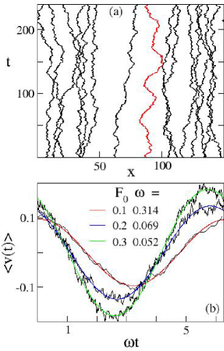
Figure 1: (Color online). Panel (a): typical SF dynamics. The tagged particle (red) is subjected to the external periodic force $F(t)=F_{0}\cos\omega t$, while the other ones perform the usual stochastic dynamics. Panel (b): Linear Response relation (18). Average velocity $\langle v(t)\rangle$ vs $\omega t$ for $k_{B}T=1.0$, $\gamma=0.5$, $\rho=0.25$ and different values of $F_{0}$ and $\omega$. Three typical numerical curves (black lines) are fitted through the relation (18), showing a linear dependence on the amplitude of the applied sinusoidal force. Averages have been taken over more than 2000 periods of each realization, performing at least 10 realizations corresponding to each $\omega$.

Let’s first define the file density at a point $x$ of the line at time $t$ as

$$\rho(x,t)=\frac{n(x,t)}{dx}$$ (4)

where $n(x,t)$ refers to the number of particles in the bin $\left[x-\frac{dx}{2},x+\frac{dx}{2}\right]$ at time $t$. It is straightforward to note that the quantity $\rho(x,t)$ is a local property of the file, independent of the relabeling of the particles due to collisions. A direct consequence of this is that the time evolution of the file profile density can be described by the Diffusion noise equation for a 1 dimensional gas of N non-interacting Brownian particles vanVliet

$$\frac{\partial}{\partial t}\rho(x,t)=-\frac{\partial}{\partial x}J(x,t),$$ (5)

having a recourse to the definition of a stochastic flux $J(x,t)=-D\frac{\partial}{\partial x}\rho(x,t)+\eta(x,t)$. The noise term $\eta(x,t)$ can be shown to be Gaussian and satisfy the following properties VKampen :

$$\begin{array}[]{l}\eta(L,t)=\eta(0,t)\\ \langle\eta(x,t)\rangle=0,\\ \langle\eta(x,t)\eta(x^{\prime},t^{\prime})\rangle=2D\delta(x-x^{\prime})\delta(t-t^{\prime})\langle\rho(x,t)\rangle,\end{array}$$ (6)

the first one of which refers to the conservation of the particle’s number (conserved noise) along the segment $[0,L]$ with periodic boundary conditions. The remaining properties in (6) are required to fulfill the equations for the first two moments of $\rho(x,t)$

$$\begin{array}[]{l}\frac{\partial}{\partial t}\langle\rho(x,t)\rangle=D\frac{\partial^{2}}{\partial x^{2}}\langle\rho(x,t)\rangle\\ \begin{split}\left[\frac{\partial}{\partial t}-D\frac{\partial^{2}}{\partial x_{1}^{2}}-D\frac{\partial^{2}}{\partial x_{2}^{2}}\right]\langle\rho(x_{1},t)\rho(x_{2},t)\rangle_{C}=\\ 2D\frac{\partial}{\partial x_{1}}\frac{\partial}{\partial x_{2}}\delta(x_{1}-x_{2})\langle\rho(x,t)\rangle,\end{split}\end{array}$$ (7)

where we made use of the short notation $\langle\rho(x_{1},t)\rho(x_{2},t)\rangle_{C}=\langle\rho(x_{1},t)\rho(x_{2},t)\rangle-\langle\rho(x_{1},t)\rangle\langle\rho(x_{2},t)\rangle$. As it is apparent from (6), the correlation function of the noise depends upon the particular solution of the diffusion equation in (7): in the following, as well as in the numerical simulations performed, we consider the case of a uniformly distributed file, namely $\langle\rho(x,0)\rangle\equiv\langle\rho(x,t)\rangle\equiv\rho$.

The connection between the dynamics of the density over $[0,L]$ and the the motion of a tagged particle in the single file system is achieved in the following way. Given two particle trajectories, $x_{1}(t)$ and $x_{2}(t)$, the number of particles between these has to remain constant in time because of the non-overlapping condition, this implies

$$\frac{d}{dt}\int_{x_{1}(t)}^{x_{2}(t)}\rho(x,t)\,dx=0.$$ (8)

Performing the derivative and making use of (5), the previous relation then reads

$$\begin{split}v_{2}(t)\rho\left(x_{2}(t),t\right)-J\left(x_{2}(t),t\right)-v_{1}(t)\rho\left(x_{1}(t),t\right)\\ +J\left(x_{1}(t),t\right)=0;\end{split}$$

now, both the terms must set to zero irrespective of the particle labels: we can thus write down the equation for the single file particle as

$$v(t)\rho\left(x(t),t\right)=J\left(x(t),t\right).$$ (9)

We notice that, although the relation (9) just introduced is exact, it is highly nonlinear. We are thus compelled to fall back upon two approximations in order to solve it. The first approximation is to assume that the density surrounding the particle position is essentially constant: $\rho(0,t)\equiv\langle\rho(0,t)\rangle\equiv\rho\,$. The second approximation we put forward is to assume that the particles movements are correlated over a range equal to the displacement of the tagged particle, such that we can take the current $J(x(t),t)$ to be equal to the current at the particles initial position. Taking this to be at $x=0$ we thus have $J(x(t),t)=J(0,t)$. Notice that similar assumptions have been superimposed by Alexander and Pincus in a previous treatment of the single file subdiffusive dynamics on a lattice Pincus .

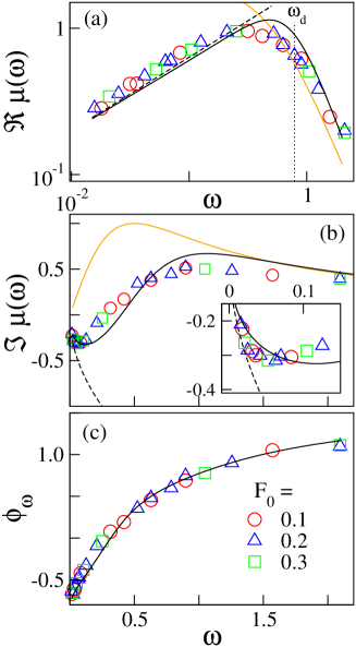
Figure 2: (Color online). Real (a) imaginary part (b) and phase (c) of $\mu{(\omega)}$ obtained through the relation (18), for different $F_{0}$ and $\omega$. Simulation parameters are the same as in Fig.1. The dashed lines represent the formula (15) and are seen to fit quite well the asymptotic subdiffusive behavior of the mobility (see the inset of panel (b) where the low-frequency behavior of $\Im\mu(\omega)$ is blown up). The initial diffusive behavior (orange lines) is responsible for the high-frequency regime $\omega\gg\omega_{d}$ (dotted line in (a)). The GLE expression for the mobility (45) furnishes a very good description of both regimes: solid black lines. The non-perfect agreement between theory and data is due to the small value of the ratio $\tau_{d}/\tau_{b}=4$ (see text and TABLE I).

With these approximations Eq.(9) gets the form

$$v(t)\simeq\frac{J(0,t)}{\rho}.$$ (10)

Moreover defining the Fourier transform (and its inverse) in the space and time domains as

$$\begin{array}[]{l}f(q,\omega)=\int_{-\infty}^{+\infty}dxdt\,f(x,t)\,e^{-i(qx-\omega t)}\\ f(x,t)=\int_{-\infty}^{+\infty}\frac{dqd\omega}{\left(2\pi\right)^{2}}\,f(q,\omega)\,e^{i(qx-\omega t)},\end{array}$$ (11)

the equation (10) can be casted as

$$v(\omega)\simeq\frac{1}{\rho}\int_{-\infty}^{+\infty}\frac{dq}{2\pi}J(q,\omega),$$

which, by means of (5) and of the definition of the stochastic flux, reads

$$v(\omega)\simeq\frac{1}{\rho}\int_{-\infty}^{+\infty}\frac{dq}{2\pi}\,\frac{-i\omega}{q^{2}D-i\omega}\,\eta(q,\omega).$$ (12)

Let us now define the following quantity

$$\mu(\omega)=\frac{1}{\rho\gamma}\int_{-\infty}^{+\infty}\frac{dq}{2\pi}\,\frac{-i\omega}{q^{2}D-i\omega};$$ (13)

using (12) and the noise properties in (6), it is readily verified that the following equality holds:

$$\langle v(\omega)v(\omega^{\prime})\rangle=2k_{B}T\,\Re\left[\mu(\omega)\right]\,2\pi\delta(\omega+\omega^{\prime}).$$ (14)

Furthermore a direct calculation of (13) gives

$$\mu(\omega)=\sqrt{\frac{2}{k_{B}T\,\gamma}}\,\frac{\sqrt{\omega}}{4\rho}\,[1-i]$$ (15)

which, substituted in (14) and consistent with the Wiener-Khintchine theorem, yields the asymptotic form of the velocity autocorrelation function (VAF) of a single file particle Marchesoni

$$\langle v(t)v(0)\rangle=-\sqrt{\frac{k_{B}T}{\gamma\,\pi}}\,\frac{1}{4\rho}\,\frac{1}{t^{3/2}}.$$ (16)

In passing from eq.(14) to (16) we implicitly adopted the convention $\langle v(t)v(0)\rangle=\langle v(-t)v(0)\rangle$, which uniquely determines the mobility $\mu(\omega)$ to be the Fourier-Laplace transform of the VAF, i.e.

$$\mu(\omega)=\frac{\int_{0}^{+\infty}\langle v(t)v(0)\rangle\,e^{i\omega t}}{k_{B}T}.$$ (17)

The relation (17) is known as the first Fluctuation-Dissipation theorem or Green-Kubo relation Kubo . However for linear systems the connection between correlation functions and mobility hinges on the domain of transport processes Zwanzig-Transport : within this framework the equations (12) and (13) on one hand, and their statistical counterpart (17) on the other, encouraged us to explore the validity of a linear response relation of the type

$$\langle v(t)\rangle=\Re\left[\tilde{\mu}(\omega)\,F_{0}e^{i\omega t}\right].$$ (18)

Indeed, applying a periodic external force $F(t)=F_{0}\cos\omega t$ to a tagged particle and leaving the remaining surrounding ones unaffected (see Fig.1(a)), the response (18) has been directly measured by meaning of extensive numerical simulations. The results are shown in Fig.1(b) and Fig.2, where the real, the imaginary part and the relative phase $\phi_{\omega}$ of the quantity $\tilde{\mu}(\omega)$ are displayed. At first we note as the average velocity depends linearly upon the force amplitude $F_{0}$ according to the equation (18). Most important, the low frequency behavior of $\tilde{\mu}(\omega)$ fully agrees with the analytical formula for the mobility $\mu(\omega)$ given in (15) (dashed line). We can interpret this result recalling that a particle undergoes a normal diffusive behavior up to a time scale $\tau_{d}=\frac{1}{D\rho^{2}}$, which is the time needed by a couple of particle to collide with one of the neighboring diffusants Marchesoni ; correspondingly we can assume that the tagged driven particle will feel the presence of the surrounding ones over frequencies smaller than the threshold $\omega_{d}=\frac{2\pi}{\tau_{d}}$ (dotted line). Conversely, for $\omega\gg\omega_{d}$, $\tilde{\mu}(\omega)$ coincide with the mobility of a free Brownian walker: $1/(\gamma-i\omega)$. The numerical results in Fig.2 can thus be summarized by writing, besides the relation (18), the mobility $\tilde{\mu}(\omega)$ as

$$\tilde{\mu}(\omega)\simeq\left\{\begin{array}[]{ccc}\frac{\gamma+i\omega}{\gamma^{2}+\omega^{2}}&&\omega\gg\omega_{d}\\ \sqrt{\frac{2}{k_{B}T\,\gamma}}\,\frac{\sqrt{\omega}}{4\rho}\,[1-i]&&\omega\ll\omega_{d}.\end{array}\right.$$ (19)

The numerical evidence of the effectiveness of a linear response relation allows us to rewrite the eq.(12) as

$$v(\omega)=\tilde{\mu}(\omega)\tilde{\xi}(\omega)$$ (20)

where the introduced noise satisfies $\langle\tilde{\xi}(t)\rangle=0$. On the other hand, its spectrum $S_{\xi}(\omega)$ exhibits two different regimes according to (19):

$$S_{\xi}(\omega)=\int_{-\infty}^{+\infty}\langle\xi(t)\xi(0)\rangle e^{i\omega t}\simeq\left\{\begin{array}[]{ccc}2k_{B}T\gamma&&\omega\gg\omega_{d}\\ \frac{\left(2k_{B}T\right)^{3/2}\sqrt{\gamma}\rho}{\sqrt{\omega}}&&\omega\ll\omega_{d}.\end{array}\right.$$ (21)

The file particles surrounding the tagged one thus act as an additional bath responsible for the onset of subdiffusional behavior. The nature of this long-ranged correlations in the noise source can be easily understood in terms of the collisional interaction between the file components. Note in fact that the expression (21) leads to a slowly decaying positive correlated noise $\langle\tilde{\xi}(t)\tilde{\xi}(0)\rangle\propto\frac{1}{\sqrt{t}}$: this non-trivial finding is the signature of constrained geometry systems. Indeed, although the collisions tend to tie back the particle motion, leading to the negative velocity correlations (16), the noise provides the way to maintain $\langle v(t)\rangle=0$ on time scale of the order $1/\gamma$. Another way to say this, is that in a collision a particle exchanges velocity and noise. Anyway, this is a manifestation of the Fluctuation-Dissipation theorem. Furthermore, the non-Markovian power-law nature of the noise spectrum characterizes the asymptotic Fractional Brownian Motion (FBM) of the tagged particle Mandelbroot .

We end this section stressing that, using the formalism so far developed, we can calculate the other asymptotic statistical properties of the system. In fact it is straightforward to write down an expression for the particle’s position similarly to what we did in (12) for its velocity:

$$x(\omega)\simeq\frac{1}{\rho}\int_{-\infty}^{+\infty}\frac{dq}{2\pi}\,\frac{\eta(q,\omega)}{q^{2}D-i\omega}.$$ (22)

For instance, making use of (22) and (12) we get

$$\langle x(\omega)v(\omega^{\prime})\rangle=\sqrt{\frac{k_{B}T}{2\gamma}}\frac{1}{\rho}\frac{i}{\sqrt{\omega}}\,2\pi\delta\left(\omega+\omega^{\prime}\right).$$ (23)

III Generalized Langevin description

In this section we will collect the results outlined in the previous one and will put them in a consistent compact formulation. We emphasize three fundamental properties that such a representation must incorporate

i) the Linear Response relation (LR) must hold: (18);

ii) the Fluctuation Dissipation theorem (FDT) is also valid: (21);

iii) all the statistical properties exhibit two different behaviors, Brownian or subdiffusive motion, depending on whether time is smaller or larger than $\tau_{d}$. We will in the following assume that the time scale $\tau_{b}=1/\gamma$ is smaller than $\tau_{d}$ such that the particles are moving diffusively (in contrast with ballistically) before colliding with each other.

Our aim is thus to write down an effective equation for the microscopic dynamics of a tagged particle in single file systems, according to $i),\,ii),\,iii)$. Such an equation turns out to be

$$\begin{array}[]{l}\dot{x}(t)=v(t)\\ \dot{v}(t)=-\left[\gamma+2\,n_{d}^{2}\,\gamma_{1/2}\,{}_{0}D_{t}^{-1/2}\right]v(t)+\tilde{\xi}(t).\end{array}$$ (24)

Several new symbols have been introduced in the previous expression deserving an explanation. Firstly the quantity $n_{d}=\frac{\gamma}{\rho\sqrt{k_{B}T}}$ plays the same role as $\tau_{d}$ in the collisional representation of the particle’s motion Marchesoni : it accounts for the number of collisions a particle suffers before attaining subdiffusive behavior. Secondly the quantity $\gamma_{1/2}$, which has the dimension of $\left[1/t^{3/2}\right]$, is the generalized damping coefficient and is equal to $\left(\frac{1}{\tau_{d}}\right)^{3/2}$ since $\tau_{d}$ is the unique relevant time scale of the system. The third symbol in (24) is the Riemann-Liouville fractional operator Samko :

$${}_{0}D_{t}^{-1/2}f(t)=\frac{1}{\Gamma\left(\frac{1}{2}\right)}\int_{0}^{t}\frac{f(t^{\prime})}{\left|t-t^{\prime}\right|^{\frac{1}{2}}}\,dt^{\prime}.$$ (25)

Note that if we use the definition of the Caputo fractional derivative  Caputo

$$\frac{d^{1/2}f(t)}{dt^{1/2}}=\frac{1}{\Gamma\left(\frac{1}{2}\right)}\int_{0}^{t}\frac{df(t^{\prime})/dt^{\prime}}{\left|t-t^{\prime}\right|^{\frac{1}{2}}}\,dt^{\prime},$$

then (24) takes the form

$$\frac{d^{2}x(t)}{dt^{2}}+\gamma\frac{dx(t)}{dt}+2\,n_{d}^{2}\,\gamma_{1/2}\,\frac{d^{1/2}x(t)}{dt^{1/2}}=\tilde{\xi}(t).$$ (26)

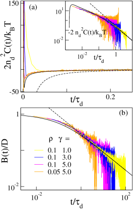
Figure 3: (Color online) Second moments of observables: Rescaled VAF $\langle v(t)v(0)\rangle$ (a) and position-velocity correlation function $\langle\left[x(t)-x(0)\right]v(t)\rangle$ (b) vs $t/\tau_{d}$ for several densities $\rho$ and damping $\gamma$. $k_{B}T=1.0$. Dashed lines are the asymptotic formulae (16) and (23) respectively, whereas the solid ones represent the GLE predictions (35) and (40) for $\rho=0.05$ and $\gamma=5.0$. To improve our statistics we averaged over 3000 different realizations.

The noise appearing in (24) satisfies the properties (21). Indeed we recall that the diffusive microscopic time scale $\tau_{b}=\frac{1}{\gamma}$ can be expressed as $\tau_{b}=\frac{\tau_{d}}{n_{d}^{2}}$ Marchesoni so that the equation (24) can be re-casted as

$$\dot{v}(t)=-\int_{0}^{t}\tilde{\gamma}\left(t-t^{\prime}\right)v(t^{\prime})\,dt^{\prime}+\tilde{\xi}(t),$$ (27)

introducing the generalized damping and defining the $\delta$ function to contribute half at the end point of an integral:

$$\tilde{\gamma}(t)=2\,\gamma\left[\delta(t)+\frac{1}{\sqrt{\pi\,\tau_{d}\,t}}\right].$$ (28)

Thence such a definition allows us to express the properties in (21) through the compact notation of the Generalized Fluctuation-Dissipation theorem Kubo

$$\langle\tilde{\xi}(t)\tilde{\xi}(t^{\prime})\rangle=k_{B}T\,\tilde{\gamma}(\left|t-t^{\prime}\right|)$$ (29)

The solution of the equation (24) can be easily achieved by means of the Laplace transform:

$$\begin{array}[]{l}x(s)=\frac{x(0)}{s}+v(0)\tilde{\psi}(s)+\tilde{\xi}(s)\tilde{\psi}(s)\\ v(s)=v(0)\tilde{\mu}(s)+\tilde{\xi}(s)\tilde{\mu}(s),\end{array}$$ (30)

where the mobility $\tilde{\mu}(t)$ in the $s-$domain is given by

$$\tilde{\mu}(s)=\frac{1}{s+\tilde{\gamma}(s)}=\frac{1}{s+\gamma+2\,n_{d}^{2}\,\gamma_{1/2}\,s^{-1/2}}$$ (31)

and

$$\tilde{\psi}(s)=\frac{\tilde{\mu}(s)}{s}=\frac{1}{s^{2}+\gamma s+2\,n_{d}^{2}\,\gamma_{1/2}\,s^{1/2}}.$$ (32)

It is immediate to verify that the expression in (31) matches the predicted two regimes in (19). In the time domain the solution of the Generalized Langevin Equation in (24) takes the simple form

$$\begin{array}[]{l}x(t)=x(0)+v(0)\tilde{\psi}(t)+\int_{0}^{t}\tilde{\xi}(t^{\prime})\tilde{\psi}(t-t^{\prime})\,dt^{\prime}\\ v(t)=v(0)\tilde{\mu}(t)+\int_{0}^{t}\tilde{\xi}(t^{\prime})\tilde{\mu}(t-t^{\prime})\,dt^{\prime},\end{array}$$ (33)

from which it is apparent that the joint probability distribution for $x$ and $v$ is a Gaussian in this formulation. Position and velocity are in fact linear functionals of $\tilde{\xi}(t)$ which is a (non-Markovian) Gaussian random process. Such a property corroborates all the previous analytical derivations for the probability distribution of a tagged particle moving subdiffusively in a single file system (see for example Ref.SF_basic and references therein) and it is clearly at odds with a Fractional Fokker-Planck description of the corresponding subdiffusive process, which leads to a stretched Gaussian solution Klafter .

Furthermore we point out that the GLE (24) correctly describes the time behavior of all the observable moments of position and velocity, not only in the long time asymptotic regime but also at the initial diffusive stage. To see this it is sufficient to start from the general solutions (33) and put in some physical assumptions Mazo . For instance the first moments of velocity and position will read

$$\begin{array}[]{l}\langle x(t)\rangle=\langle x(0)\rangle+\langle v(0)\rangle\tilde{\psi}(t)\\ \langle v(t)\rangle=\langle v(0)\rangle\tilde{\mu}(t).\end{array}$$ (34)

The second moments, however, are more interesting quantities: for the VAF, assuming $\langle v^{2}(0)\rangle=k_{B}T$, it is straightforward to prove

$$C(t)\equiv\langle v(t)v(0)\rangle=k_{B}T\,\tilde{\mu}(t)$$ (35)

which is the Generalized First Kubo theorem. The numerical evidence of this is given in Fig.3(a), where several rescaled curves are plotted against the analytic function in (35) after numerical inversion of the mobility in (31).

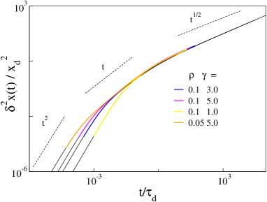
Figure 4: (Color online) Mean square displacement $\delta x^{2}(t)=\Sigma_{i=1}^{N}\left[x_{i}(t)-x_{i}(0)\right]^{2}/N$ for different values of $\rho$ and $\gamma$ with $k_{B}T=1.0$ plotted versus $t/\tau_{d}$. Data have been rescaled by $x_{d}^{2}=2/\left(\rho^{2}\sqrt{\pi}\right)$ on y axis Marchesoni . The black solid lines represent the theoretical predictions as given by the GLE formula (36): they provide an excellent description of the three diffusive regimes. Data have been averaged over 30 different realizations for N of the order of $10^{4}$.

The excellent agreement between the analytical description yielded by (24) and the numerical data is even more apparent looking at the mean square displacement of the tagged particle (Fig.4). Indeed from (33) one obtains

$$\delta x^{2}(t)\equiv\langle\left[x(t)-x(0)\right]^{2}\rangle=2\,\langle v^{2}(0)\rangle\int_{0}^{t}\tilde{\psi}(t^{\prime})\,dt^{\prime},$$ (36)

where it is possible to recognize the theorem stated in Ref.Marchesoni provided that

$$\frac{d}{dt}\tilde{\psi}(t)=\tilde{\mu}(t).$$ (37)

The exact expression given in (36) quantitatively reproduces the three stages of the $\delta x^{2}(t)$ curves in Fig.4 (ballistic, diffusive, subdiffusive) as well as the characteristic time scales ($\tau_{b}$ and $\tau_{d}$) on which the crossovers between them take place

$$\delta x^{2}(t)=\left\{\begin{array}[]{ccc}k_{B}T\,t^{2}&&t\ll\tau_{b}\\ 2D\,t&&\tau_{b}\ll t\ll\tau_{d}\\ 2\sqrt{\frac{D}{\pi\rho^{2}}}\sqrt{t}&&t\gg\tau_{d}.\end{array}\right.,$$ (38)

An analytical inversion of the formula in (32) including the crossover to the subdiffusive regime can be achieved by neglecting the inertial (ballistic) term leading to

$$\langle\left[x(t)-x(0)\right]^{2}\rangle\simeq\frac{1}{\rho^{2}}\left[\sqrt{\frac{4t}{\pi\tau_{d}}}+\frac{e^{\frac{4t}{\tau_{d}}}}{2}\,\mathrm{erfc}\left(\sqrt{\frac{4t}{\tau_{d}}}\right)-\frac{1}{2}\right]$$ (39)

In general we believe the GLE (24) provides a very good description of the tagged particle’s stochastic motion only when the condition $\tau_{b}\ll\tau_{d}$ is fulfilled (see TABLE I). In other words the particle must attain a truly diffusive regime before getting a collision with one of its nearest neighbors. One can see that the proposed GLE cannot work well in the opposite case where $\tau_{b}>\tau_{d}$ since all interactions with neighboring particles vanish according to Eq. (24) as $\gamma\to 0$. This cannot be true, since the particle will still collide and exchange momentum with its neighbors even though the rest of the friction with the surroundings vanish. We have not found a GLE that works well in the case $\tau_{b}>\tau_{d}$.

$\rho$	$\gamma$	$\tau_{b}$	$\tau_{d}$	$\tau_{d}/\tau_{b}$
0.25	0.5	2.0	8.0	4
0.1	1.0	1.0	100	100
0.1	3.0	$\sim$0.334	300	900
0.1	5.0	0.2	500	2500
0.05	5.0	0.2	2000	10000

Table 1: Values of $\tau_{\rm b}$, $\tau_{\rm d}$ and their ratio for the values of $\rho$ and $\gamma$ used in Figs. 2, 3, 4, and 5.

The close comparison between theory and numerics when $\tau_{b}\ll\tau_{d}$ is also displayed by the position-velocity correlation function $\langle x(t)v(t)\rangle$ for which the following expression holds

$$B(t)\equiv\langle\left[x(t)-x(0)\right]v(t)\rangle=\langle v^{2}(0)\rangle\,\tilde{\psi}(t)$$ (40)

In Fig.3(b) we compare the numerical data with both (40) and (23), which is expected to work well only in the asymptotic regime.

The relaxation of the second moment of the velocity $\langle v^{2}(t)\rangle$ to the asymptotic value $k_{B}T$ is given by

$$\langle v^{2}(t)\rangle=\langle v^{2}(0)\rangle\,\mu^{2}(t)+k_{B}T\,\left[1-\mu^{2}(t)\right],$$ (41)

and deserves particular attention. In Ref. Lutz it has been shown that the Fractional Brownian process  Mandelbroot generated by a Fractional Langevin equation and the stochastic process corresponding to the relative Fractional Kramer equation  Barkay are on average the same, except for the second moment of the velocity. We point out that such a discrepancy is a common problem in non-equilibrium statistical mechanics, whenever one is concerned to pass from a Generalized Langevin dynamical description of a non-Markovian process  Mori to the corresponding Fokker-Planck equation for the probability distribution  Zwanzig (see for instance the discussion in Ref. Chang on the inconsistency of a retarded Fokker-Planck equation of the Rubin model  Rubin ). In the GLE (24) the $\langle v^{2}(t)\rangle$ relaxation process is dictated by the Brownian dynamics (see Fig. 5) as long as $\tau_{b}\ll\tau_{d}$. The Fractional Kramer equation corresponding to (24) would read

$$\frac{\partial P(x,v,t)}{\partial t}+v\,\frac{\partial P(x,v,t)}{\partial x}$$

$$\quad\quad=\left[\gamma+\gamma_{1/2}\,{}_{0}D_{t}^{-1/2}\right]\hat{L}_{FP}P(x,v,t),$$ (42)

where $\hat{L}_{FP}=\frac{\partial}{\partial v}v+k_{B}T\frac{\partial^{2}}{\partial v^{2}}$. In the $\tau_{b}\ll\tau_{d}$ limit the $\langle v^{2}(t)\rangle_{FKE}$ expression yielded by (42) is the one provided by the usual Fokker-Planck, i.e. $\langle v^{2}(t)\rangle_{FKE}\simeq k_{B}T\,e^{-2\gamma t}$ once $v(0)=0$, in agreement with the exponential saturation shown in Fig. 5. This could lead to believe that the GLE description (24) and the Kramer Eq.(42) are de facto equivalent in the range $\tau_{b}\ll\tau_{d}$. Nevertheless we expect that the $P(x,t)$ solution of (42) is still a stretched exponential instead of a Gaussian: this fundamental difference casts some general doubt on the possibility to determine a Fokker-Planck equation for systems whose microscopic dynamics is represented by a FLE.

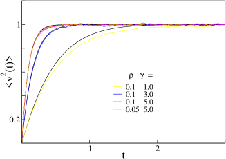
Figure 5: (Color online). Second moment of the velocity $\langle v^{2}(t)\rangle$ vs $t$, displayed for several densities $\rho$ and damping $\gamma$. $k_{B}T=1.0$. The initial tagged particle velocity $v(0)$ has been set to 0. The expression (41) (solid black lines) shows the typical Brownian exponential relaxation to $k_{B}T$: for all the displayed curves $\tau_{b}/\tau_{d}\ll 1$. To improve our statistics we averaged the numerical curves over 3000 realizations.

The last part of this section is devoted to the property $i)$, namely the validity of LR. In the presence of an external force acting from time equal zero and onwards, (24)-(27) takes the form

$$\begin{array}[]{l}\dot{x}(t)=v(t)\\ \dot{v}(t)=-\int_{0}^{t}\tilde{\gamma}\left(t-t^{\prime}\right)v(t^{\prime})\,dt^{\prime}+F(t)+\tilde{\xi}(t).\end{array}$$ (43)

The LR (18) in $s-$space can thus expressed by using (31) as

$$\langle v(s)\rangle=\tilde{\mu}(s)F(s),$$ (44)

so that , thanks to the expression (31), the real and imaginary part of the mobility $\tilde{\mu}(t)$ read

$$\begin{array}[]{l}\Re\left[\tilde{\mu}(\omega)\right]=\frac{\gamma+\sqrt{2}\,n_{d}^{2}\,\gamma_{1/2}\omega^{-1/2}}{\left(\gamma+\sqrt{2}\,n_{d}^{2}\,\gamma_{1/2}\omega^{-1/2}\right)^{2}+\left(\sqrt{2}n_{d}^{2}\,\gamma_{1/2}\omega^{-1/2}-\omega\right)^{2}}\\ \Im\left[\tilde{\mu}(\omega)\right]=\frac{\omega-\sqrt{2}n_{d}^{2}\,\gamma_{1/2}\omega^{-1/2}}{\left(\gamma+\sqrt{2}\,n_{d}^{2}\,\gamma_{1/2}\omega^{-1/2}\right)^{2}+\left(\sqrt{2}n_{d}^{2}\,\gamma_{1/2}\omega^{-1/2}-\omega\right)^{2}}\end{array}$$ (45)

Remarkably, in Fig. 2 both functions (45) (solid black lines) are shown to fit quite well the outcome of our numerics.

Finally in the case of a constant external force, i.e. $F(t)=F$ for $t\geq 0$ in (43), the LR provides that the drift $\langle x(t)\rangle_{F}$ satisfies the Generalized Einstein relation

$$\langle x(t)\rangle_{F}=\langle x(0)\rangle+F\,\frac{\delta x^{2}(t)}{2\,k_{B}T}$$ (46)

that has been shown to be valid on file systems moving on a ring Ferrari and on an infinite one-dimensional lattice Oshanin .

IV Conclusion

In this paper we introduced the effective equation ruling the microscopic stochastic motion of a SF tagged particle. Starting from a diffusion-like formalism for the file density dynamics, we were led to several properties for which the GLE (24)-(27) can be regarded as a representation. Indeed the GLE formalism provides an elegant representation of Generalized Fluctuation-Dissipation theorems (29)-(35), Linear Response (44) and Generalized Einstein relation (46), all remarkable properties satisfied by the particle, both in its diffusive and in subdiffusive phase.

Nevertheless we want to stress that the GLE is just a description, though very good, of the stochastic motion of the SF particle and, in this perspective, is valid within certain limits. However, along the same line, within certain approximations the Langevin Equation provides an excellent effective equation for the motion of a Brownian particle immersed in a thermal bath, i.e. it describes well the ballistic and diffusive regimes of the particle, but one would not expect it to be exact in the region of crossover between the two regimes. In SF systems the tagged particle is subjected to two types of thermal baths, as is apparent from (24): the first is mimicked by the usual Markovian uncorrelated noise, whereas the second, physically embodied by the surrounding file’s particles, is achieved by the introduction of an additional non-Markovian term, responsible for the strong memory effects. Surprisingly this “sum of thermal baths” turns out to be well described (in the same manner as for the Brownian particle/LE) by simply the algebraic sum of two independent terms in the stochastic equation of motion. Alternatively one could view (24) as an usual LE (3) where the relabeling-collisional symmetry accounts for the fractional term.

Acknowledgments

We are indebted with Prof. Mehran Kardar for having deeply influenced this work. We also like to thank Prof. Fabio Marchesoni and Tobias Ambjörnsson for several useful discussions. A.T. is grateful to acknowledge the “Angelo Della Riccia” foundation for having supported this work. M.A.L. thanks the Danish National Research Foundation for support via a grant to MEMPHYS - Center for Biomembrane Physics.

References

- (1) T. E. Harris, J. Appl. Prob. 2, 323 (1965).
- (2) D. G. Levitt, Phys. Rev. A 8 3050(1973); J. K. Percus, Phys. Rev. A 9, 557 (1974); K. Hahn and J. Kärger, J. Phys. A: Math. Gen. 28, 3061 (1995); C. Rödenbeck et al, Phys. Rev. E 57, 4382 (1998); M. Kollmann, Phys. Rev. Lett. 90, 180602 (2003); L. Lizana and T. Ambjörnsson, Phys. Rev. Lett. 100, 200601 (2008).
- (3) P. M. Richards, Phys. Rev. B 16, 1393 (1977); J. Kärger et al, J. of Catal. 136, 283 (1992); K. Hahn and J. Kärger, J. Phys. Chem. 100, 316 (1996); D. S. Sholl and K. A. Fichthorn, Phys. Rev. E, 55, 7753 (1997); K. K. Mon and J. K. Percus, J. Chem. Phys. 119, 3343 (2003).
- (4) U. Hong et al., Zeolites 11, 816 (1991); D. S. Sholl and K. A. Fichthorn, Phys. Rev. Lett. 79, 3569 (1997); P. Demontis et al., J. Chem. Phys. 120, 9233 (2004); P. Demontis et al., Microp. Mesop. Mat. 86, 166 (2005).
- (5) J. Kärger and M. Ruthven, Diffusion in Zeolites and in Other Microporous Solids (Wiley, New York, 1992).
- (6) D. J. Aidley and P. R. Standfield, Ion Channels: Molecules in Action (Cambridge University Press, New York, 1996).
- (7) B. Alberts et al., Molecular Biology of the Cell (Garland, New York, 1994).
- (8) J. Kärger, Phys. Rev. A 45, 4173 (1992); A. Taloni and F. Marchesoni, Phys. Rev. Lett. 96, 020601 (2006).
- (9) Q. H. Wei et al., Science 287, 625 (2000); B. Cui et al., Phys. Rev. Lett. 89, 188302 (2002). C. Lutz et al., Phys. Rev. Lett. 93, 026001 (2004).
- (10) J. Kärger et al., Microp. Mat. 3, 401 (1995). V. Gupta et al., Chem. Phys. Lett. 247, 596 (1995); K. Hahn et al., Phys. Rev. Lett. 76, 2762 (1996).
- (11) R. Kutner et al., Phys. Rev. B 30, 4382 (1984); H. Hahn and J. Kärger, J. Chem. Phys. B 102, 5766 (1998); H. L. Tepper et al., J. Chem. Phys. 110, 11511 (1999); K. K. Mon and J. K. Percus, J. Chem. Phys. 117, 2289 (2002); S. Savel’ev et al, Phys. Rev. E 74, 021119 (2006).
- (12) D. Kumar, Phys. Rev. E 78, 021133 (2008).
- (13) H. van Beijeren et al, Phys. Rev. B 28, 5711 (1983).
- (14) F. Marchesoni and A. Taloni, Phys. Rev. Lett. 97, 106101 (2006); A. Taloni and F. Marchesoni, Phys. Rev. E 74, 051119 (2006).
- (15) R. Metzler and J. Klafter, Phys. Rep. 339, 1 (2000).
- (16) Y. Kantor and M. Kardar, Phys. Rev. E 76, 061121 (2007).
- (17) J. Chuang et al., Phys. Rev. E, 65, 011802 (2001); Y. Kantor and M. Kardar, Phys. Rev. E 69, 021806 (2004);
- (18) A. Rosso and M. Kardar, to be submitted (2008).
- (19) P. G. de Gennes, J. Chem. Phys. 55, 572 (1971).
- (20) Y. Imry and B. Gavish, J. Chem. Phys. 61, 1554 (1974); M. Büttiker and R. Landauer, J. Phys. C: Solid St. Physics 13, L325 (1980); M. Büttiker and R. Landauer, Phys. Rev. B 24, 4079 (1981).
- (21) H. Mori, J. Phys. Soc. Japan 11, 1029 (1956); H. Mori, Prog. Theor. Phys. 33, 423 (1965); H. Mori, Prog. Theor. Phys. 34, 399 (1965).
- (22) R. Kubo, Rep. Progr. Phys. 29, 255 (1966).
- (23) E. Lutz, Phys. Rev. E 64, 051106 (2001).
- (24) N. Laskin, Physica A 287, 482 (2000); S. C. Kou and X. S. Xie, Phys. Rev. Lett. 93, 180603 (2004); A. Dubkov and B. Spagnolo, Fluct. Noise Lett. 5, L267 (2005); W. Min et al., Phys. Rev. Lett. 94, 198302 (2005); S. Chaudhury et al., J. Phys. Chem. B 111, 2377 (2007); B. J. West and S. Picozzi, Phys. Rev. E 65, 037106 (2002); S. Picozzi and B. J. West, Phys. Rev. E 66, 046118 (2002).
- (25) D. W. Jepsen, J. Math. Phys. 6, 405 (1965); J. L. Lebowitz and J. K. Percus, Phys. Rev. 122, 155 (1967).
- (26) K. M. van Vliet, J. Math. Phys. 12, 1981 (1971).
- (27) N. G. van Kampen, Stochastic Processes in Physics and Chemistry (North-Holland, Amsterdam, 1981).
- (28) S. Alexander and P. Pincus, Phys. Rev. B 18, 2011 (1978).
- (29) R. Zwanzig, Ann. Rev. Phys. Chem. 16, 67 (1965).
- (30) S. G. Samko et al., Fractional Integrals and Derivatives, Theory and Applications (Gordon and Breach, Amsterdam, 1993).
- (31) M. Caputo, Geophys. J. R. Astr. Soc. 13, 529 (1967); M. Caputo, Elasticità e Dissipazione (Zanichelli, Bologna, 1969).
- (32) B. B. Mandelbroot and J. W. Van Ness, SIAM Rev. 10, 422 (1968).
- (33) R. M. Mazo in Stochastic Processes in Nonequilibrium Systems, edited by L. Garrido, P. Seglar and P. J. Shepherd, (Springer-Verlag, New York, 1965); J. M. Porrà et al., Phys. Rev. E 53, 5872 (1996).
- (34) E. Barkai and R. J. Silbey, J. Phys. Chem. B 104, 3866 (2000).
- (35) R. Zwanzig, Phys. Rev. 124, 983 (1961); S. Nordholm and R. Zwanzig, J. Stat. Phys. 13, 347 (1975).
- (36) R. J. Rubin, J. Math. Phys. 1, 309 (1960); R. J. Rubin, J. Math. Phys. 2, 373, (1961); H. Nakazawa, Suppl. Prog. Theor. Phys. 36, 172 (1966); J. M. Deutch and R. Silbey, Phys. Rev. A 3, 2049 (1971).
- (37) E. L. Chang et al., Mol. Phys. 28, 997 (1974).
- (38) P. Ferrari et al. in Statistical Physics and Dynamical Systems, edited by J. Fritz, A. Jaffe and D. Szasz, (Birkhäusen, Boston, 1985).
- (39) S. F. Burlatsky et al., Phys. Rev. E 54, 3165 (1996).