Heat wave propagation in a nonlinear chain

Abstract

We investigate the propagation of temperature perturbations in an array of coupled nonlinear oscillators at finite temperature. We evaluate the response function at equilibrium and show how the memory effects affect the diffusion properties. A comparison with nonequilibrium simulations reveals that the telegraph equation provides a reliable interpretative paradigm for describing quantitatively the propagation of a heat pulse at the macroscopic level. The results could be of help in understanding and modeling energy transport in individual nanotubes.

I Introduction

The propagation of temperature fluctuations under nonequilibrium conditions may display significant deviations from a simple diffusive behavior. As it is know  Joseph and Preziosi (1989), heat can propagate in a wavelike form on time scales comparable with some typical relaxation time. This is accounted for by suitable extensions of the standard Fourier’s law to include, for example, a finite response time for the heat current. On the other hand, it is of primary interest to derive such a phenomenological laws from microscopic dynamics. In this respect, much work has been performed recently, mostly on simplified models, with the goal of understanding nonequilibrium heat–conducting states from first principles  Lepri et al. (2003). Much emphasis has been put on violations of Fourier’s law in the stationary case  Lepri et al. (2003) as well as in describing anomalous heat diffusion  Cipriani et al. (2005). Transient heat propagation has received much less attention  Zhao (2006); Delfini et al. (2007). As a matter of fact, the spreading of the energy perturbation field, yield complementary information on how heat propagates through the system Helfand (1960) and provides useful insight on the nature of heat carrying excitations.

Besides those fundamental issues, there is a growing interest in understanding how heat is transported at the nanoscale  Cahill et al. (2003). In this context, carbon nanotube materials are of special relevance due to their exceptionally high thermal conductivity related to their quasi one-dimensional vibrational structure  Hone et al. (1999); Yu et al. (2005). Recently, Osman and Srivastava  Osman and Srivastava (2005) investigated the propagation of intense heat pulses in single–walled carbon nanotubes by means of molecular dynamics. They observed that, together with pulses traveling with the sound velocity, a secondary and slower peak can also propagate as a ”second sound” type of wave  Chester (1963). Shiomi and Maruyama Shiomi and Maruyama (2006), argued that this should be related to relatively fast optical phonons, that due to the quasi one–dimensional structure, have very long relaxation times and thus contribute to wavelike heat propagation.

It is thus relevant to study simplified models that can help to understand better the conduction properties. In this respect, an example is the length dependence of conductivity in carbon and boron-nitride nanotubes which has been very recently observed experimentally Chang et al. (2008). Indeed, experimental data are compatible with scaling laws theoretically predicted for simple nonlinear models. In this spirit, in the present paper we analyze the heat pulse propagation in a classical lattice model, a chain of classical, harmonically coupled, oscillators with a quartic pinning (on-site) potential. In particular, we compare the linear-response predictions with nonequilibrium molecular dynamics.

The paper is organized as follows. In Sec. II we introduce the microscopic one-dimensional model. After some general considerations about linear response we present the response functions as computed from molecular dynamics simulations (Sec. III). Based on the numerical data, we introduce an approximated (single-pole) form for the response that leads to the telegraph equation for the temperature–field evolution. This equation, along the phenomenological values of its parameters, is precious to compare with nonequilibrium simulations. The transient evolution of a temperature pulse is investigated in Sec. IV. Qualitative and quantitative deviations from the behavior expected for the simple telegraph equation are highlighted.

II The nonlinear chain

The model consists of an anharmonic chain of $N$ particles (each with unit mass) whose displacements are denoted by $u_{i}$:

$$\ddot{u}_{i}=-u_{i}-u_{i}^{3}+C(u_{i+1}-2u_{i}+u_{i-1})\quad.$$ (1)

In the linear approximation, where the cubic force term is dropped, the eigenfrequencies $\Omega$ of the associated normal modes are expressed as a function of the wavenumber $q$ by

$$\Omega^{2}(q)\;=\;1+2C(1-\cos q)\quad.$$ (2)

The units have been fixed in such a way to have a unitary gap in the spectrum. With this choice the only free parameters of the model are the energy per particle $\epsilon=E/N$ and the coupling constant $C$.

Several numerical studies (see e.g. Ref. Hu et al., 1998 and Aoki and Kusnezov, 2000 as well as Ref.  Lepri et al., 2003 and the bibliography within) clarified, that for models like (1) the thermal conductivity is finite, and that a diffusive heat propagation is expected at long times. However, on time scales which are of the order of the energy current relaxation time some wave-like transient behavior could be expected. However, a rigorous derivation of a macroscopic transport law from the microscopic equations of motion, especially for small systems in a low-dimensional environment, remains a formidable challenge.

To conclude this Section we mention that the we limit ourselves here to the case of a single-well on-site potential. The double-well case has been studied in Ref. Flach and Mutschke, 1994. A detailed analysis of second sound propagation in the three-dimensional lattice is given in Ref. Schneider and Stoll, 1978.

III Linear response

At a coarse-grained level, the most general linear constitutive relation between the energy current $J(x,t)$ and the local temperature gradient can be written as an extension of the usual Fourier law (we limit ourselves for simplicity to a one-dimensional case),

$$J(x,t)\;=\;-\int_{-\infty}^{\infty}dx^{\prime}\int_{-\infty}^{t}dt^{\prime}K(x-x^{\prime},t-t^{\prime})\frac{\partial T}{\partial x}(x^{\prime},t^{\prime})\quad.$$ (3)

Substituting into the continuity equation, and assuming a decay of the kernel $K$ at infinity, one obtains

$$\frac{\partial T}{\partial t}\;=\;\int_{-\infty}^{\infty}dx^{\prime}\int_{-\infty}^{t}dt^{\prime}K(x-x^{\prime},t-t^{\prime})\frac{\partial^{2}T}{\partial x^{2}}(x^{\prime},t^{\prime})$$ (4)

(up to the heat capacity). The generalized heat diffusion equation is formally solved by means of the Fourier-Laplace transform, with the convention

$$f(q,z)\equiv\frac{1}{\sqrt{2\pi}}\int_{-\infty}^{\infty}dx\int_{0}^{\infty}dt\,f(x,t)e^{-i(qx-zt)}\quad,$$ (5)

yielding

$$T(q,z)=\frac{T_{0}(q)}{-iz+q^{2}K(q,z)}\quad,$$ (6)

with $T_{0}$ being the initial condition. The standard diffusive pole is recovered for a constant $K(q,z)=D$, i.e. for an instantaneous response, with $D$ being the thermal diffusivity. The simplest improvement would be to include a single relaxation time $\tau$, and no spatial memory effects, namely an exponentially decaying kernel in time of the Cattaneo-Vernotte type  Joseph and Preziosi (1989). In the above notation this means choosing a single-pole response of the form

$$K(q,z)\;=\;\frac{v^{2}}{-iz+1/\tau}\quad.$$ (7)

The quantity $v$ has the physical dimensions of a velocity, is defined as  Joseph and Preziosi (1989)

$$v=\sqrt{\frac{D}{\tau}}\quad.$$ (8)

Substituting approximation (7) into Eq. (6) one can readily recognize that the resulting $T(q,z)$ is nothing but the Laplace transform of the equation

$$\frac{\partial^{2}T}{\partial t^{2}}+\frac{1}{\tau}\frac{\partial T}{\partial t}=v^{2}\frac{\partial^{2}T}{\partial x^{2}}\quad.$$ (9)

This is known as the telegraph equation  Joseph and Preziosi (1989). The equation contains an additional term with respect to the standard heat equation that affects the solution for times of order $\tau$. Indeed, the second-order derivative with respect to time leads to a finite velocity of perturbations. For instance, for a pulse initially localized at the origin, $T=0$ at distances $|x|>vt$. For $t\gg\tau$, ordinary diffusive behavior is recovered Morse and Feshbach (1953). It should be also remembered, that Eq. (9) arises as a continuum limit of the persistent random walk (see Ref. Weiss, 2002 and references within).

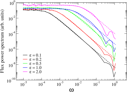
Figure 1: Power spectrum of energy current for a chain of $N=4096$ $C=1$ and different energies. Dashed lines are best fit with a Lorentzian line-shape $a/(1+\tau^{2}\omega^{2})$.

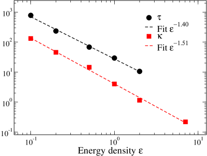
Figure 2: The relaxation time $\tau$ as a function of energy for $N=2048$, $C=1$. The dashed line is a power-law fit.

According to the fluctuation–dissipation theorem  Chaikin and Lubensky (1995) the imaginary part of the response function $K(q,\omega)$ is proportional to $\omega$ times the equilibrium power spectrum of the observable that couples to the external field. In the case of a temperature gradient, the observable to consider is the energy current, whose microscopic expression for model (1) reads  Lepri et al. (2003)

$$j_{n}=-\frac{C}{2}(\dot{u}_{n+1}+\dot{u}_{n})(u_{n+1}-u_{n})\quad.$$ (10)

In order to test for the validity of approximation (7) we have first of all evaluated the power spectra of the $q=0$ component of the flux, $j(q=0,t)=\sum_{n}j_{n}$ from molecular dynamics. To this aim, we have performed microcanonical simulations by integrating Eqs. (1) (with periodic boundary conditions, $u_{n}=u_{n+N}$) by means of a fourth–order symplectic algorithm  Mclachlan and Atela (1992). Initial conditions were chosen with the particles at equilibrium. Their velocities were drawn at random from a Gaussian distribution and rescaled by suitable factors to assign the total energy per particle $\epsilon$ to the prescribed value and to set the total initial momentum equal to zero. A suitable transient is elapsed before data acquisition for statistical averaging. Conservation of energy and momentum was monitored during each run. The chosen time–steps (0.05–0.1) ensures energy conservation better then a few parts per million. The reliability of the spectra has been checked against different choices of the run duration and sampling times.

Fig. 1 reports $\langle|j(q=0,\omega)|^{2}\rangle$, where the average is performed over about 100 trajectories. The data show that, in agreement with Eq. (7), the spectra are fitted very well by a single Lorentzian over a wide range of energies and frequencies. The relaxation time decreases as a power of the energy density, $\tau\sim\epsilon^{-\beta}$ with $\beta\approx 1.4$ (Fig. 2). To compute the velocity $v$ we measured independently the thermal conductivity $\kappa$ by the standard Green-Kubo formula i.e. by integrating the flux autocorrelation in the time domain Lepri et al. (2003). It turns out that the diffusivity $D$ is approximately equal to the thermal conductivity since the heat capacity is very close to one in our units (it varies only by a few percent in the considered energy range). As shown again in Fig. 2, $\kappa$ decreases as a power of the energy density. This is in agreement with previous work on related models  Aoki and Kusnezov (2000); Aoki et al. (2006). The corresponding exponent is very close to $\beta$ meaning the that $v$ as defined by Eq. (8) is roughly constant.

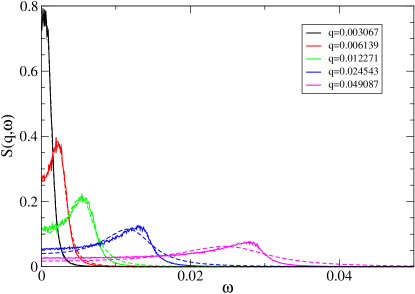
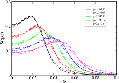
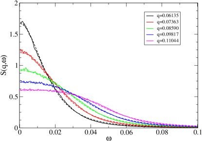
Figure 3: Power spectrum of energy fluctuations for a chain of $N=2048$ $C=1$ and (a) $\epsilon=0.1$ (b) $\epsilon=0.5$ and (c) $\epsilon=1.0$. Dashed lines are best fit with Eq.(14).

In a second series of simulations, we computed the dynamical structure factor, namely the square modulus of temporal Fourier transform of the energy density on the lattice

$$e_{n}=\frac{\dot{u}_{n}^{2}}{2}+\frac{u_{n}^{2}}{2}+\frac{u_{n}^{4}}{4}+\frac{C}{2}(u_{n+1}-u_{n})^{2}$$ (11)

$$e(q,t)\;=\;\frac{1}{N}\,\sum_{n}\,e_{n}\exp(-iqn)\quad,$$ (12)

which is defined as

$$S(q,\omega)\;=\;\big{\langle}\big{|}e(q,\omega)\big{|}^{2}\big{\rangle}\quad.$$ (13)

The square brackets denote an average over a set of independent molecular–dynamics runs. By virtue of the periodic boundaries, the allowed values of the wavenumber $q$ are integer multiples of $2\pi/N$.

The data in Fig. 3 are representative of the numerical results. At low enough temperatures we see a peak at finite-frequency which suggests some kind of oscillating response i.e. the propagation of damped temperature–waves. Upon increasing $\epsilon$ and/or decreasing $q$, the spectra display a central peak, akin to the one of an overdamped oscillator which signals the onset of diffusive behavior.

For not too large $q$ the spectra are well fitted by a Lorentzian shape

$$S(q,\omega)=\frac{S_{0}}{(\omega^{2}-\omega^{2}_{0}(q))^{2}+({\omega}/{\tau(q)})^{2}}\quad.$$ (14)

We found that the dependence of the parameters $\omega_{0}(q)$ and $\tau(q)$ from the wavenumber $q$ is

$$\omega_{0}(q)\;=\;c|q|\quad,\qquad\frac{1}{\tau(q)}=\frac{1}{\tau}\left[1+\left|\frac{q}{q_{0}}\right|\right]$$ (15)

where $c$ and $q_{0}$ are fitting parameters (see Fig. 4).

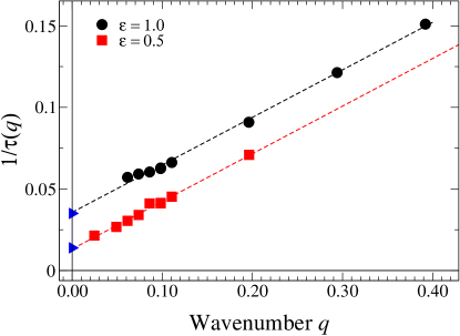
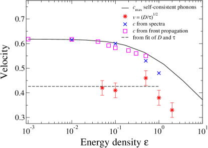
Figure 4: (a) Dependence of $\tau(q)$ on the wavenumber for two different energy densities. Lines are best fit with the law (15). Triangles are the data for $\tau$ reported Fig. 2. (b) Comparison of the relevant velocities emerging from linear response. The velocity $c$ defined from Eq. (14) (dots) is very close to the maximum group velocity computed from the effective dispersion, Eq. (16) (solid line). The thermal velocity $v$ is defined by Eq. (8) (see text). Data are obtained for a chain of length $N=2048$ with $C=1$.

The observed form of the line-shape, Eq. (14), is fully consistent with what expected from Eq. (9). However, the origin of the dependence of $\tau(q)$ cannot be accounted for by the simplified kernel (7) and is presumably a signature of spatial correlations. Nonetheless, we note that the value $\tau$ obtained by extrapolating at $q\to 0$ in the second of Eqs. (15) is in very good agreement with the value measured from flux spectra (see again Fig 2). Another important quantitative difference is in the characteristic velocities. In Fig. 4b we compare the velocity $c$ from the fitting (15) with $v$ as given by definition (8). Since we found above that $D$ and $\tau$ are both proportional to (roughly) the same power-law $\epsilon^{-\beta}$, in Fig. 4 we report also the ratio of the corresponding proportionality constants. The measured values of $v$ in Fig. (4) show that $v\lesssim c$ in the considered range.

We may surmise that the velocity $c$ should be related to the group velocity of the harmonic waves. To account for finite-temperature effects we have computed the renormalized dispersion relation in the self–consistent phonon approximation  Dauxois et al. (1993),

$$\tilde{\Omega}^{2}(q)\;=\;\omega^{2}(T)+2C(1-\cos q)\quad.$$ (16)

where

$$\omega^{2}(T)=1+\frac{\langle u^{4}\rangle}{\langle u^{2}\rangle}$$ (17)

The second and fourth momenta of the displacements have been evaluated numerically. The data for $c$ are very close to the maximum group velocity $c_{max}$, namely the largest value of $d\tilde{\Omega}(q)/dq$ as computed from formula (16), see Fig. 4.

We conclude that, although the telegraph equation (9) accounts for the line-shape of the energy correlators, there are, at least in the considered times and length ranges, some quantitative deviations. The fact that $v$ and $c$ are different can be partly understood by noting that $v$ is associated with diffusive processes and results from interaction of all possible lattice waves. The maximum group velocity $c$ will thus be an upper bound to $v$, but the two need not be equal Joseph and Preziosi (1989). It is interesting to mention that differences in the measured velocities were previously reported also in a model of hard–point particles  Delfini et al. (2007) .

IV Heat pulse propagation

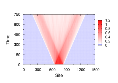
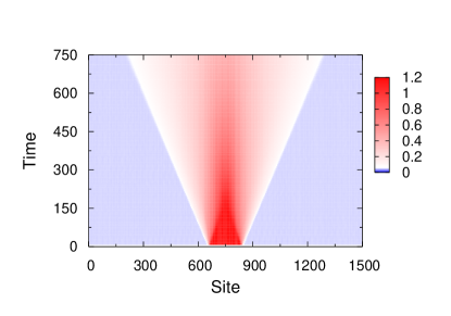
Figure 5: Spatio-temporal density maps of the normalized temperature profiles $T(n,t)/T_{0}$ of two heat pulses propagating in chains at temperatures $T_{b}=0.001$ (a) and $T_{b}=0.04$ (b). Other parameters are: $T_{0}=20\times T_{b}$, $C=1$, $N=1500$.

The linear response results reported so far suggest that the propagation of heat waves could be described at the macroscopic level, at least for small enough energies, through the telegraph equation (9). In order to test this conjecture, we performed nonequilibrium numerical simulations where a heat pulse of temperature $T_{0}$ is excited in a small region of width $\Delta N$ within a chain otherwise at equilibrium at the bulk temperature $T_{b}<T_{0}$ and observed as it evolves. A typical pulse experiment proceeds as follows. First the chain is let evolve at a fixed energy $\epsilon=T_{b}$ for a long enough equilibration time. Subsequently, the portion $[(N-\Delta N)/2,(N+\Delta N)/2]$ is put in contact with a Langevin thermostat at the temperature $T_{0}$, while the rest of the chain is kept frozen in its equilibrium configuration. When the heated portion has reached thermal equilibrium with the thermostat, the latter is removed and the equations of motion of the whole chain are integrated at constant energy. For the pulse propagation experiments we used the symplectic “Position Extended Forest-Ruth Like” (PEFRL) algorithm of Omelyan et al. Omelyan et al. (2002) and a velocity Verlet algorithm for the microcanonical and Langevin integrations, respectively. Furthermore, since we used free-ends boundary conditions, we took care to chose the integration time so as to avoid the propagating pulse to be reflected at the chain edges. In order to obtain highly accurate results, we averaged the time-dependent temperature profiles over a large ensemble of ${\mathcal{N}}$ independent realizations of the equilibrium configuration of both the bulk and the excited regions of the chain. All results reported in the following were obtained with ${\mathcal{N}}=2\times 10^{4}$ and $\Delta N=90$, except where explicitly indicated otherwise.

Typical spatio-temporal portraits of the temperature profiles describing the evolution of a heat pulse are reported in Fig. 5 for two different values of the bulk temperature. For small values of $T_{b}$, the heat excitation gives rise to two symmetrical pulses, traveling in opposite directions at a constant speed. Such speed is extremely close to the maximum group velocity of the linear modes, $c_{max}=0.618$. As the bulk temperature is increased, the correlation time $\tau$ is expected to decrease thus reducing the window of ballistic propagation. In fact, a diffusion-like evolution of the pulse is observed already at $T_{b}=0.04$ (Fig. 5b). However, it can be clearly appreciated that the bulk temperature is still not sufficiently large for the pulse to spread homogeneously at all heights. At a closer inspection, it is not difficult to realize that the the front baseline still clearly moves at a constant speed close to $c_{max}$.

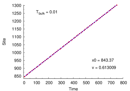
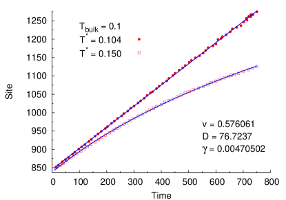
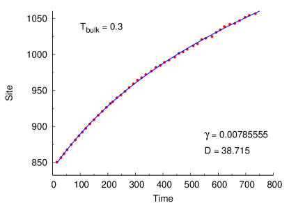
Figure 6: Analysis of heat pulse propagation. Spatio-temporal contour maps of the normalized temperature profiles $T(n,t)/T_{0}$ (left panels) and time variation of the front baseline position at a given temperature height: $T^{\ast}=0.0105$ (b), $T^{\ast}=0.104$ and $T^{\ast}=0.15$ (d), $T^{\ast}=0.35$ (f). Parameters are. $C=1$, $T_{b}=0.01$ (a) and (b), $T_{b}=0.1$ (c) and (d), $T_{b}=0.3$ (e) and (f), $T_{0}=20\times T_{b}$, $C=1$, $N=1500$. The straight lines in panels (b) and (c) are linear fits, while the other solid lines are fits with formula (19).

Stated more precisely, our conjecture implies that, if the telegraph equation holds, then the motion of the heat pulse front should carry the information on the microscopic parameters that enter the continuum description, namely the speed $v$ and the correlation time $\tau$ (see again equation (9)). Let us imagine to cut the time-dependent temperature profiles that describe the chain dynamics after excitation of the heat pulse at a given temperature $T^{\ast}$, with $T_{b}<T^{\ast}\ll T_{0}$. Then, one may extract useful information by tracking the sites occupied by the pulse front at the height $T^{\ast}$ during its evolution. In other words, one may study the trajectories defined implicitly as

$$T(x(t),t)=T^{\ast}$$ (18)

where $T(n,t)=\langle\dot{u}^{2}_{n}(t)\rangle$ is the temperature field , the average being computed over an ensemble of ${\mathcal{N}}$ independent trajectories. If $T^{\ast}$ is sufficiently close to the bulk temperature $T_{b}$, the linear response results should hold, and the persistent random walk should be recovered, namely

$$x(t)-x_{0}\simeq\sqrt{\frac{2v^{2}}{\gamma}\left[t-\frac{1}{\gamma}\left(1-e^{-\gamma t}\right)\right]}$$ (19)

The analysis summarized in Fig. 6 proves the validity of our inference. Close to the background temperature, the propagation crosses-over from ballistic to diffusive on a time scale that is well predicted by the equilibrium simulations (see Fig. 2). For $T_{b}=0.01$, the equilibrium prediction would be a time scale of the order $1/\gamma\approx 2\times 10^{4}$. Correspondingly, on our observation window we observe purely ballistic propagation (upper right panel of Fig. 6). Conversely, for $T_{b}=0.3$ the equilibrium relaxation time is about 150. Accordingly, we indeed observe a crossover to diffusion within the time span of our simulations. From the fit we get $1/\gamma=127$, in good agreement with the equilibrium prediction (lower right panel of Fig. 6). At intermediate temperatures, an increase of the cut temperature height in the vicinity of $T_{b}$ causes the ballistic/diffusive cross-over to occur on shorter time scales, as expected since the relaxation time approaches the observation time. In fact, this can be seen as the very definition of the intermediate time scale. This is clearly illustrated in the middle right panel of Fig. 6 ($T_{b}=0.1$), where the transition becomes visible in the simulation time window upon raising the cut temperature from $T^{\ast}=0.104$ to $T^{\ast}=0.15$.

As a further check of consistency, we have examined the time-variations of the temperature field second moment $\mu_{2}(t)$, defined as

$$\mu_{2}(t)=\sum_{n}(n-\langle n\rangle)^{2}z_{n}$$ (20)

where $z_{n}=\dot{u}^{2}/\sum_{m}\dot{u}^{2}_{m}$ and $\langle n\rangle=\sum_{n}nz_{n}$. However, straight calculation of the second moment from its definition requires extremely accurate averages, due to the strong amplification of the fluctuations in the bulk regions away from $\langle n\rangle$. For this reason, in order to monitor $\mu_{2}$ over time, two copies of the system were evolved starting from identical initial conditions but for the small region around the center of the chain, where the heat pulse is generated. An accurate estimate of the pulse spread for finite values of $T_{b}$ can then be obtained from the second moment of the difference between the profiles of the two system clones.

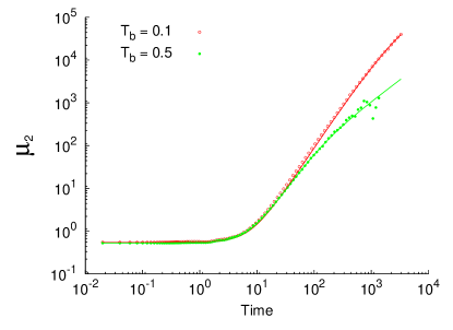
Figure 7: Time evolution of the second moment of the temperature field for two values of the bulk temperature, $T_{b}=0.1$ ($T_{0}=0.5$) and $T_{b}=0.5$ ($T_{0}=1.0$) (symbols) and two-parameter fits with expression (21). The initial conditions $\mu_{2}(0)$ have been fixed at the corresponding values extracted from the numerics. Other parameters are: $C=1$, $N=5000$, $\Delta N=10$.

The result of such procedure is shown in Fig. 7 for two values of the bulk temperature in the case of a narrow excitation. As it shows, the heat pulse spreads according to the prescription of the telegraph equation, that is

$$\mu_{2}(t)=\mu_{2}(0)+\frac{2v^{2}}{\gamma}\left[t-\frac{1}{\gamma}\left(1-e^{-\gamma t}\right)\right]$$ (21)

The time scales extracted from the fits are $\tau=917.5$ ($T_{b}=0.1$) and $\tau=53.9$ ($T_{b}=0.5$) . These figures are in good agreement with the equilibrium relaxation times that we found by fitting the results of microcanonical simulations (data shown in Fig. 2), $\tau=760.8$ ($T_{b}=0.1$) and $\tau=76.2$ ($T_{b}=0.5$).

The best-fit values of the velocities $v$ prove rather insensitive to the bulk temperature. We find $v=0.095$ ($T_{b}=0.1$) and $v=0.1$ ($T_{b}=0.5$). Interestingly, these values are smaller than all estimates shown in Fig. 4. This is likely to reflect the temperature-dependence of the relaxation times at different heights within the pulse. For a finite temperature disturbance, the fronts do not spread at the same rate, causing the hotter portions to lag behind the advancing baseline. Overall, this should reflect in a lower value of the pulse velocity during its first ballistic stage.

V Discussion

In this report we have investigated the relaxation of temperature fluctuations in a discrete nonlinear chain. At low temperatures the relaxation time $\tau$ of the energy current must be taken into account, leading to correction to the standard diffusive behavior. Starting from numerical calculation of the response function and to the simplest level of approximation, we obtained the telegraph equation, Eq. (9), and estimated the temperature dependence of its parameters.

The comparison between the linear-response prediction and the nonequilibrium simulations reveals that the telegraph equation provides a reliable macroscopic interpretative framework for quantifying the front propagation. In particular, we have shown that the second moment of the temperature field displays the ballistic/diffusive cross-over on a time scale in accordance with the correlation times of energy fluctuations extracted from equilibrium simulations. The same is true for the front propagation at temperatures close to the background. It might be surmised that this type of macroscopic description should apply to all models displaying normal energy transport, such as chains of coupled rotors or other one-dimensional models with pinning potentials Lepri et al. (2003), or three-dimensional systems Volz et al. (1996).

By following the propagation at higher temperatures, the front appears to smear out in the course of time. It is likely that this effect could be captured by a kernel of the Jeffreys type, as shown by Maruyama and co-workers Shiomi and Maruyama (2006). Another possible improvement would be to include spatial memory effects, by allowing for a space-dependence memory dependence in the kernel $K$, Eq.(3). This is especially important if one wishes to describe systems with anomalous transport properties Lepri et al. (2003). Indeed, in this case heat propagation is quantitatively described by a Levy walk process Cipriani et al. (2005); Delfini et al. (2007), which is precisely the generalization of the persistent random walk for of a memory decaying as a power law. As a consequence, the macroscopic equation generalizing the telegraph equation should involve mixed spatio-temporal fractional derivatives  Sokolov and Metzler (2003). Possible nonlinear heat-wave propagation could also be taken into account by including higher–order powers of the local gradient. Further work along these lines is in progress.

Finally, we remark that our results confirm that wave-like transport of energy is associated with the presence of optical branches in the linear spectrum. This could be of interest for heat transport in single-walled carbon nanotubes, where a significant contribution of optical phonons to wave-like conduction has been reported Shiomi and Maruyama (2006). In this respect one may conjecture that our simplified model may provide an effective description of more complex quasi-one-dimensional nanostructures.

References

- Joseph and Preziosi (1989) D. D. Joseph and L. Preziosi, Rev. Mod. Phys. 61, 41 (1989).
- Lepri et al. (2003) S. Lepri, R. Livi, and A. Politi, Phys. Rep. 377, 1 (2003).
- Cipriani et al. (2005) P. Cipriani, S. Denisov, and A. Politi, Phys. Rev. Lett. 94, 244301 (2005).
- Zhao (2006) H. Zhao, Phys. Rev. Lett. 96, 140602 (2006).
- Delfini et al. (2007) L. Delfini, S. Denisov, S. Lepri, R. Livi, P. K. Mohanty, and A. Politi, Europ. Phys. J. - Special Topics 146, 21 (2007).
- Helfand (1960) E. Helfand, Phys. Rev. 119, 1 (1960).
- Cahill et al. (2003) D. G. Cahill, W. K. Ford, K. E. Goodson, G. D. Mahan, A. Majumdar, H. J. Maris, R. Merlin, and S. R. Phillpot, J. App. Phys. 93, 793 (2003).
- Hone et al. (1999) J. Hone, M. Whitney, C. Piskoti, and A. Zettl, Phys. Rev. B 59, R2514 (1999).
- Yu et al. (2005) C. Yu, L. Shi, Z. Yao, D. Li, and A. Majumdar, Nano Letters 5, 1842 (2005).
- Osman and Srivastava (2005) M. A. Osman and D. Srivastava, Phys. Rev. B 72, 125413 (2005).
- Chester (1963) M. Chester, Phys. Rev. 131, 2013 (1963).
- Shiomi and Maruyama (2006) J. Shiomi and S. Maruyama, Phys. Rev. B 73, 205420 (2006).
- Chang et al. (2008) C. W. Chang, D. Okawa, H. Garcia, A. Majumdar, and A. Zettl, Phys. Rev. Lett. 101, 075903 (2008).
- Hu et al. (1998) B. Hu, B. Li, and H. Zhao, Phys. Rev. E 57, 2992 (1998).
- Aoki and Kusnezov (2000) K. Aoki and D. Kusnezov, Phys. Lett. A 265, 250 (2000).
- Flach and Mutschke (1994) S. Flach and G. Mutschke, Phys. Rev. E 49, 5018 (1994).
- Schneider and Stoll (1978) T. Schneider and E. Stoll, Phys. Rev. B 18, 6468 (1978).
- Morse and Feshbach (1953) P. M. Morse and H. Feshbach, Methods of Theoretical Physics (McGraw-Hill, New York, 1953).
- Weiss (2002) G. Weiss, Physica D 311, 381 (2002).
- Chaikin and Lubensky (1995) P. M. Chaikin and T. Lubensky, Principles of Condensed Matter Physics (Cambridge University Press, Cambridge, 1995).
- Mclachlan and Atela (1992) R. I. Mclachlan and P. Atela, Nonlinearity 5, 541 (1992).
- Aoki et al. (2006) K. Aoki, J. Lukkarinen, and H. Spohn, J. Stat. Phys. 124, 1105 (2006).
- Dauxois et al. (1993) T. Dauxois, M. Peyrard, and A. R. Bishop, Phys. Rev. E 47, 684 (1993).
- Omelyan et al. (2002) I. Omelyan, I. Mryglod, and R. Folk, Computer Physics Communications 146, 188 (2002).
- Volz et al. (1996) S. Volz, J.-B. Saulnier, M. Lallemand, B. Perrin, P. Depondt, and M. Mareschal, Phys. Rev. B 54, 340 (1996).
- Sokolov and Metzler (2003) I. M. Sokolov and R. Metzler, Phys. Rev. E 67, 010101 (2003).