Integrable hydrodynamics of Calogero-Sutherland model: Bidirectional Benjamin-Ono equation.

Abstract

We develop a hydrodynamic description of the classical Calogero-Sutherland liquid: a Calogero-Sutherland model with an infinite number of particles and a non-vanishing density of particles. The hydrodynamic equations, being written for the density and velocity fields of the liquid, are shown to be a bidirectional analogue of Benjamin-Ono equation. The latter is known to describe internal waves of deep stratified fluids. We show that the bidirectional Benjamin-Ono equation appears as a real reduction of the modified KP hierarchy. We derive the Chiral Non-linear Equation which appears as a chiral reduction of the bidirectional equation. The conventional Benjamin-Ono equation is a degeneration of the Chiral Non-Linear Equation at large density. We construct multi-phase solutions of the bidirectional Benjamin-Ono equations and of the Chiral Non-Linear equations.

1 Introduction

The Calogero-Sutherland model (CSM) [1, 2] describes particles moving on a circle and interacting through an inverse $\sin$-square potential. The Hamiltonian of the model reads

$${\cal H}_{CSM}=\frac{1}{2}\sum_{j=1}^{N}p_{j}^{2}+\frac{1}{2}\left(\frac{\pi}{L}\right)^{2}\sum_{j,k=1;j\neq k}^{N}\frac{g^{2}}{\sin^{2}\frac{\pi}{L}(x_{j}-x_{k})},$$ (1)

where $x_{j}$ are coordinates of $N$ particles, $p_{j}$ are their momenta, and $g$ is the coupling constant. We took the mass of the particles to be unity. The momenta $p_{j}$ and coordinates $x_{j}$ are canonically conjugate variables.

The model (classical and quantum) occupies an exceptional place in physics and mathematics and has been studied extensively. It is completely integrable. Its solutions can be written down explicitly as finite dimensional determinants (for review see [3]).

In the limit of a large period $L\to\infty$ the CSM degenerates to its rational version – Calogero (aka Calogero-Moser) model (CM) where the pair-particle interaction is $1/{x^{2}}$. The CSM itself is a degeneration of the elliptic Calogero model, where the pair particle interaction is given by the Weierstrass $\wp$-function of the distance. In this paper we discuss the classical trigonometric model (1) commenting on the rational limit when appropriate.

We are interested in describing a Calogero-Sutherland liquid, i.e., the system (1) in thermodynamic limit when $N\to\infty$ and $L\to\infty$ while the average density $N/L$ is kept constant. We assume that the limit exists and that in this limit a microscopic density and current fields

$$\rho(x,t) = \sum_{j=1}^{N}\delta(x-x_{j}(t)),$$ (2)

$$j(x,t) = \sum_{j=1}^{N}p_{j}(t)\delta(x-x_{j}(t))$$ (3)

are smooth single-valued real periodic functions with a period $L$ equal to the period of the potential . In this case the system will be described by hydrodynamic equations written on the density field $\rho(x,t)$ and the velocity field $v(x,t)$. The velocity is defined as $j=\rho v$.

The hydrodynamic approach is a powerful tool to study the evolution of smooth features with typical size much larger than the inter-particle distance. Apart from application to the CSM, the hydrodynamic equations obtained in this paper are interesting integrable equations. We show that they are new real reductions of the modified Kadomtzev-Petviashvili equation (MKP1).

In this paper we consider a classical system, however the approach developed below can be extended to the quantum case $\{p_{j},\,x_{k}\}=\delta_{jk}\rightarrow[p_{j},\,x_{k}]=i\hbar\delta_{jk}$ almost without changes. For a brief description of the hydrodynamics of the quantum system see Ref. [4]. The hydrodynamics of the quantum Calogero model has been studied previously [5, 6] in the framework of the collective field theory and some of the results below can be obtained in a classical limit (see [7]) of the quantum counterparts of Refs. [5, 6].

The outline of this paper is the following. In Sec. 2 we parameterize the particles of CSM as poles of auxiliary complex fields so that the motion of particles is encoded by evolution equations for fields. In Sec. 3 we derive a hydrodynamic limit of these equations - continuity and Euler equations with a particular form of specific enthalpy. We will refer to these equations as to the bidirectional Benjamin-Ono equation or 2BO. We present the Hamiltonian form of 2BO in Sec. 4. In Sec. 5 we discuss the bilinear form of 2BO and its relation to MKP1. In Sec. 6 we obtain the Chiral Non-Linear equation (CNL) - chiral reduction of 2BO and discuss some of its properties. In Sec. 7 we construct multi-phase and multi-soliton solutions of 2BO and CNL as a real reduction of MKP1. These solutions correspond to collective excitations of the original many-body system. Some technical points are relegated to the appendices.

2 Particles as poles of meromorphic functions

The Equations of motion of the CSM are readily obtained from the Hamiltonian (1)

$$\dot{x}_{j} = p_{j},$$ (4)

$$\dot{p}_{j} = -g^{2}\frac{\partial}{\partial x_{j}}\sum_{k=1\,(k\neq j)}^{N}\left(\frac{\pi}{L}\cot\frac{\pi}{L}(x_{j}-x_{k})\right)^{2}.$$ (5)

We rewrite this system in an equivalent way as

$$i\frac{\dot{w}_{j}}{w_{j}} = \frac{g}{2}\left(\frac{2\pi}{L}\right)^{2}\left(\sum_{k=1}^{N}\frac{w_{j}+u_{k}}{w_{j}-u_{k}}-\sum_{k=1\,(k\neq j)}^{N}\frac{w_{j}+w_{k}}{w_{j}-w_{k}}\right),\quad j=1,\dots,N$$ (6)

$$-i\frac{\dot{u}_{j}}{u_{j}} = \frac{g}{2}\left(\frac{2\pi}{L}\right)^{2}\left(\sum_{k=1}^{N}\frac{u_{j}+w_{k}}{u_{j}-w_{k}}-\sum_{k=1\,(k\neq j)}^{N}\frac{u_{j}+u_{k}}{u_{j}-u_{k}}\right),\quad j=1,\dots,N,$$ (7)

where $w_{j}(t)=e^{i\frac{2\pi}{L}x_{j}(t)}$ are complex coordinates lying on a unit circle, while $u_{j}(t)=e^{i\frac{2\pi}{L}y_{j}(t)}$ are auxiliary coordinates. Indeed, differentiating (6) with respect to time and using (6,7) to remove first derivatives in time one obtains equations equivalent to (4,5).

We note that while the coordinates $x_{j}$ are real, i.e., $|w_{j}|=1$, the auxiliary coordinates, $y_{j}(t)$, are necessarily complex. Given initial data as real positions and velocities $x_{j}(0)$ and $\dot{x}_{j}(0)$ one can find complex $y_{j}$ from (6) and then initial complex velocities $\dot{y}_{j}(0)$ from (7). Once $x_{j}$ and $\dot{x}_{j}$ are chosen to be real they will stay real at later times, even though coordinates $y_{i}$ are moving in a complex plane.

The coordinates $w_{j}(t)$ and $u_{j}(t)$ determine an evolution of two functions

$$u_{1}(w) = g\frac{\pi}{L}\sum_{j=1}^{N}\frac{w+w_{j}}{w-w_{j}}=-ig\sum_{j=1}^{N}\frac{\pi}{L}\cot\frac{\pi}{L}(x-x_{j}),\quad w=e^{i\frac{2\pi}{L}x},$$ (8)

$$u_{0}(w) = -g\frac{\pi}{L}\sum_{j=1}^{N}\frac{w+u_{j}}{w-u_{j}}=ig\sum_{j=1}^{N}\frac{\pi}{L}\cot\frac{\pi}{L}(x-y_{j}),\quad w=e^{i\frac{2\pi}{L}x}.$$ (9)

The latter functions play a major role in our approach. These are rational functions of $w$ regular at infinity and having particle coordinates as simple poles with equal residues $2\pi g/L$.

The condition that the coordinates of particles $x_{j}$ are real yields Schwarz reflection condition for the function $u_{1}$ with respect to the unit circle

$$\overline{u_{1}(w)}=-u_{1}(1/\bar{w})\qquad\mbox{or}\qquad\overline{u_{1}(x)}=-u_{1}(\bar{x}),$$ (10)

where bar denotes complex conjugation. The values of $u_{1}(w)$ in the interior and exterior of a unit circle are related by Schwarz reflection.

Comparing (6), (4) and (9) we notice that while the function $u_{1}(w)$ encodes the positions of particles $w_{j}$, the function $u_{0}(w)$ encodes the momenta of particles as its values at particle positions $w_{j}$

$$p_{j}=u_{0}(w_{j})+g\frac{\pi}{L}\sum_{k=1\,(k\neq j)}^{N}\frac{w_{j}+w_{k}}{w_{j}-w_{k}}.$$ (11)

We notice here that the positions of the particles fully determine the imaginary part of the field $u_{0}$ on a unit circle. Indeed, we have from (11)

$$\mbox{Im}\,u_{0}(x_{j})=g{\sum_{k\neq j}}\frac{\pi}{L}\cot\frac{\pi}{L}(x_{j}-x_{k}).$$ (12)

We now introduce complex functions

$$u=u_{0}+u_{1},\quad\tilde{u}=u_{0}-u_{1}.$$ (13)

One can show that they obey the equation

$$u_{t}+\partial_{x}\left[\frac{1}{2}u^{2}+i\frac{g}{2}\partial_{x}\tilde{u}\right]=0.$$ (14)

Indeed substituting the pole ansatz (8,9) into (14) and comparing the residues at poles $w_{j}$ and $u_{j}$ one arrives at (6,7).

The equation (14) connects two complex functions $u_{0}$ and $u_{1}$. The equation is equivalent to the modified Kadomtzev-Petvisashvili equation (or simply MKP1). We will discuss its relation to MKP1 in Sec. 5.

However, being complemented by the Schwarz reflection condition (10), analyticity requirements, and an additional reality requirement it becomes an equation uniquely determining $u_{0}$ and $u_{1}$ through their initial data.

The analyticity requirements read: $u_{0}(w)$ is analytic in a neighborhood of a unit circle $|w|=1$, while $u_{1}$ is analytic inside $|w|<1$ and outside $|w|>1$ of the unit circle, approaching a constant at $w\to\infty$. An additional reality requirement is the relation between the imaginary part of $u_{0}$ on a unit circle and $u_{1}$ stemming from the condition (12). We formulate and discuss these conditions in Sec. 3.3 and Sec. 5.

We will refer to the equation (14) as the bidirectional Benjamin-Ono equation (2BO). It is a bidirectional (having both right and left moving waves) generalization of the conventional Benjamin-Ono equation (BO) arising in the hydrodynamics of stratified fluids [8]. We discuss its hydrodynamic form in the next section.

The solution of (14) given by (8,9) is the CSM many body system with a finite number of particles (1). Other solutions describe CSM fluids. They are the central issue of this paper.

To conclude this section we make the following comment. The function $u_{1}$ can be expressed solely in terms of the microscopic density of particles (2) as

$$u_{1}(w)=-\pi g\oint\frac{d\zeta}{2\pi i\zeta}\,\frac{\zeta+w}{\zeta-w}\,\rho(\zeta).$$ (15)

The integral in this formula goes over the unit circle $\zeta=\exp\left(i\frac{2\pi}{L}x\right)$. In the following we will denote for brevity $\rho(\zeta)$ as $\rho(x)$, when $\zeta$ lies on a unit circle $\zeta=e^{i\frac{2\pi}{L}x}$. The density itself can be obtained as a difference of limiting values of the field $u_{1}$ at the real $x$ (on the unit circle). The discontinuity of $u_{1}$ on the unit circle gives a microscopic density (2) of particles

$$u_{1}(x+i0)-u_{1}(x-i0) = -2\pi g\rho(x),\quad\mbox{Im}\,x=0,\quad 0<\mbox{Re}\,x<L.$$ (16)

3 Hydrodynamics of Calogero-Sutherland liquid

3.1 Density and velocity

We assume that in the thermodynamic limit $N,L\to\infty$, $N/L=const$ the poles of the function $u_{1}$ are distributed along the real axis with a smooth density $\rho(x)$ and consider a complex field $u_{1}(w)$ given by formula (15). Notice that $u_{1}(w)$ defined by (15) is analytic everywhere outside of the real axis of $x$ (everywhere off the unit circle in $z$-plane) approaching a constant as $z\to\infty$. It also satisfies the reality condition (10) (the density $\rho(x)$ is real). In the thermodynamic limit the function $u_{1}$ is not a rational function anymore. It is discontinuous across the real axis with the discontinuity related to the density of particles by (16). The value of the field $u_{1}(x)$ on a real axis (on a unit circle in $z$ plane) depends on whether one approaches the real axis from above or below (unit circle from the interior $z\to e^{i\frac{2\pi}{L}(x+i0)}$ or from the exterior $z\to e^{i\frac{2\pi}{L}(x-i0)}$). More explicitly, we have from (15)

$$u_{1}(x\pm i0)=\pi g(\mp\rho+i\rho^{H}).$$ (17)

The superscript $H$ in the second term of (37) denotes the Hilbert transform and is defined as (see A for definitions and some properties of the Hilbert transform)

$$f^{H}(x)=\mathchoice{{\vbox{\hbox{$\textstyle-$}}\kern-4.86108pt}}{{\vbox{\hbox{$\scriptstyle-$}}\kern-3.25pt}}{{\vbox{\hbox{$\scriptscriptstyle-$}}\kern-2.29166pt}}{{\vbox{\hbox{$\scriptscriptstyle-$}}\kern-1.875pt}}\!\int_{0}^{L}\frac{dy}{L}\,f(y)\cot\frac{\pi}{L}(y-x).$$ (18)

We also assume that in $N\to\infty$ limit the complex field $u_{0}(w)$ remains analytic in the vicinity of the real axis in $x$-plane (i.e., in the vicinity of a unit circle in $z$-plane).

The 2BO (14) does not explicitly depend on the number of particles $N$. It holds also in thermodynamic limit $N,L\to\infty$, $N/L=const$, however solutions describing a liquid are not rational functions any longer.

We can use 2BO to define velocity through the continuity equation

$$\rho_{t} + \partial_{x}(\rho v)=0.$$ (19)

The discontinuity of the complex field $u(x)$ (13) across the real axis, as well as a discontinuity of the field $u_{1}$ (see (16)) is the density

$$u(x+i0)-u(x-i0)=u_{1}(x+i0)-u_{1}(x-i0)=-2\pi g\rho(x).$$ (20)

Differentiating (20) with respect to time and using 2BO (14) we obtain the continuity equation and identify the velocity field $v(x)$ as

$$v(x) = u_{0}(x)+\frac{1}{2}\left(u_{1}(x+i0)+u_{1}(x-i0)\right)-ig\partial_{x}\log\sqrt{\rho}(x)$$ (21)

$$= u_{0}(x)+ig\left(\pi\rho^{H}(x)-\partial_{x}\log\sqrt{\rho}(x)\right)$$

or

$$u_{0}(x)=v-ig\left(\pi\rho^{H}-\partial_{x}\log\sqrt{\rho}\right).$$ (22)

Since $v(x)$ is a real field (22) provides a reality condition analogous to (12). Indeed, one can see from (22) that

$$\mbox{Im}\,u_{0}(x)=-g\left(\pi\rho^{H}-\partial_{x}\log\sqrt{\rho}\right),$$ (23)

i.e., the imaginary part of $u_{0}(x)$ is completely determined by the density of particles or equivalently by the field $u_{1}$. It is also convenient to have an expression for $u(x)$ on a real axis

$$u(x\pm i0)=v+g\left(\mp\pi\rho+i\partial_{x}\log\sqrt{\rho}\right).$$ (24)

It has the same discontinuity across the real axis as $u_{1}(x)$.

3.2 Hydrodynamic form of 2BO.

Now we are ready to cast the equation (14) into hydrodynamic form.

Taking the real part of 2BO (14) on the real axis and using identifications (17,22) and the continuity equation, (19), after some algebra we arrive at the Euler equation

$$v_{t} + \partial_{x}\left(\frac{v^{2}}{2}+w(\rho)\right)=0,$$ (25)

with specific (per particle) enthalpy or chemical potential given by

$$w(\rho)=\frac{1}{2}(\pi g\rho)^{2}-\frac{g^{2}}{2}\frac{1}{\sqrt{\rho}}\,\partial_{x}^{2}\sqrt{\rho}+\pi g^{2}\rho_{x}^{H}.$$ (26)

Equations (19,25) are the continuity and Euler equations of classical Calogero-Sutherland model. They are the classical analogues of quantum hydrodynamic equations that have been obtained for the quantum CSM in Refs. [5, 6, 9] first using collective field theory approach [10, 11, 12] and later by the pole ansatz similar to the one used above [4]. It was noticed in [12] and then in [7] that the system (19,25,26) has a lot of similarities with classical Benjamin-Ono equation [13]. The similarities and differences with Benjamin-Ono equation are discussed below. We will refer to (19,25,26) as to a hydrodynamic form of the bidirectional Benjamin-Ono equation (2BO).

3.3 Bidirectional Benjamin-Ono equation (2BO).

Let us now summarize the 2BO equation:

$$u_{t}+\partial_{x}\left[\frac{1}{2}u^{2}+i\frac{g}{2}\partial_{x}\tilde{u}\right]=0,$$ (27)

$$u=u_{0}+u_{1},\quad\tilde{u}=u_{0}-u_{1}.$$ (28)

The functions $u_{0}$ and $u_{1}$ are subject to analyticity conditions

$$u_{1}(x)\qquad\mbox{- analytic for}\;\;\mbox{Im}\,(x)\neq 0,$$ (29)

$$u_{0}(x)\qquad\mbox{- analytic for}\;\;|\mbox{Im}\,(x)|<\epsilon\;\;\mbox{for some}\;\;\epsilon>0,$$ (30)

and to reality conditions

$$\overline{u_{1}(x)}=-u_{1}(\bar{x}).$$ (31)

In addition, the fact that the equation (27) holds in the upper half plane and in the lower half plane (inside and outside of the unit circle) yields the condition

$$\mbox{Im}\,[u(x\pm i0)]=\frac{g}{2}\partial_{x}\log\mbox{Re}\,[u_{1}(x\pm i0)].$$ (32)

It also follows from (17,23,24). The condition (32) looks more “natural” in the bilinear formulation (see eq. (56) below).

These reality and analyticity conditions reduce two complex fields $u_{0}$ and $u_{1}$ to two real fields - density $\rho(x)$ and velocity $v(x)$ as (17,22). Then, a complex equation (14) defined in both half planes immediately yields the hydrodynamic equations (19,25,26). Inversely, knowing real periodic fields $\rho(x)$ and $v(x)$ one can find fields $u_{0},u_{1}$ everywhere in a complex $x$-plane.

Mode expansion

The analyticity and reality conditions can be recast in the language of mode expansions. It follows from (15) that

$$u_{1}(w)=\left\{\begin{array}[]{lr}-\pi g\left(\rho_{0}+2\sum_{n=1}^{\infty}\rho_{n}w^{n}\right),\quad|w|<1\\ \pi g\left(\rho_{0}+2\sum_{n=1}^{\infty}\rho_{n}^{\dagger}w^{-n}\right),\quad|w|>1\end{array}\right.$$ (33)

where $\rho_{n}=\rho^{\dagger}_{-n}=\int_{0}^{L}\frac{dx}{L}\,\rho(x)e^{-i\frac{2\pi n}{L}x}$ are Fourier components of the density.

The values of the field $u_{1}(w)$ in the upper and lower half-planes are then automatically related by Schwarz reflection (10).

Conversely, the field $u_{0}(x)$ being analytic in a strip around the unit circle is represented by Laurent series

$$u_{0}(w)=V_{0}+\sum_{n=1}^{\infty}\left(a_{n}w^{n}+b_{n}w^{-n}\right),\quad|\mbox{Im}\,\log w|<2\pi\epsilon/L.$$ (34)

The 2BO equation remains intact in the case of rational degeneration. Rational degeneration of formulas of the Sec. 2 are obtained by a direct expansion in $1/L$ . In this limit fields are defined microscopically as $u_{1}(x)=-ig\sum_{j}\frac{1}{x-x_{j}}$ and $u_{0}(x)=ig\sum_{j}\frac{1}{x-y_{j}}$.

4 Hamiltonian form of 2BO

The 2BO is a Hamiltonian equation. Let us start with its Hamiltonian formulation in the hydrodynamic form $\rho_{t}=\left\{H,\rho\right\},\;v_{t}=\left\{H,v\right\}$ with the canonical Poisson bracket of density and velocity fields

$$\left\{\rho(x),v(y)\right\}=\delta^{\prime}(x-y).$$ (35)

Equations (19,25,26) follow from

$$H = \int dx\,\left(\frac{\rho v^{2}}{2}+\rho\epsilon(\rho)\right),$$ (36)

$$\epsilon(\rho) = \frac{g^{2}}{2}(\pi\rho^{H}-\partial_{x}\log\sqrt{\rho})^{2}.$$ (37)

Here the “internal energy” (37) and the enthalpy (26) are related by a general formula $w(\rho)=\frac{\delta}{\delta\rho(x)}\int dx\,\rho\epsilon(\rho)$.

For references we will give alternative expressions for the Hamiltonian. Let $\Psi=\sqrt{\rho}e^{i\vartheta}$ where $v=g\partial_{x}\vartheta$ then

$$H=\frac{g^{2}}{2}\int\left|\partial_{x}\Psi-\pi\rho^{H}\Psi\right|^{2}dx,$$ (38)

where $\rho=|\Psi|^{2}$. The Poisson’s brackets for $\Psi(x)$ are canonical: $\left\{\Psi(x),\Psi(y)\right\}=0$, and $\left\{\Psi(x),\Psi^{\star}(y)\right\}=\frac{i}{g}\delta(x-y)$. The equations of motion for $\Psi$ and $\Psi^{\star}$ are

$$\frac{i}{g}\partial_{t}\Psi=\left[-\frac{1}{2}\partial_{x}^{2}+\frac{\pi^{2}}{2}|\Psi|^{4}+\pi\left(|\Psi|^{2}\right)^{H}_{x}\right]\Psi$$ (39)

and its complex conjugate. A simple change of a dependent variable $\Phi=\Psi e^{i\pi\int^{x}dx^{\prime}\,|\Psi(x^{\prime})|^{2}}$ leads to

$$\frac{i}{g}\partial_{t}\Phi=\left[-\frac{1}{2}\partial_{x}^{2}+i2\pi\left(|\Phi|^{2}\right)^{+}_{x}\right]\Phi,$$ (40)

where $f^{+}$ denotes the function analytical in the upper half-plane of $x$ defined as $f^{+}=\frac{f-if^{H}}{2}$. One can recognize in (40) the intermediate nonlinear Schrödinger equation (INLS) which appeared in Ref.[14] as an evolution of the modulated internal wave in a deep stratified fluid. Therefore, one can alternatively think of 2BO as the hydrodynamic form of (40) identifying hydrodynamic fields $\rho$ and $v$ to be

$$\Phi=\sqrt{\rho}\exp\left\{\frac{i}{g}\int^{x}dx^{\prime}\,(v+\pi g\rho)\right\}$$ (41)

or with the field $u(x)$ from (24) as

$$ig\partial_{x}\log\Phi^{\star}=u(x-i0).$$ (42)

The Hamiltonian (36) or (38) can be rewritten in terms of $\Phi$ as

$$H=\frac{g^{2}}{2}\int\left|\partial_{x}\Phi-i2\pi\rho^{+}\Phi\right|^{2}dx,$$ (43)

where $\rho=|\Phi|^{2}$. However, the Poisson’s brackets for $\Phi$ are not canonical anymore.

2BO is an integrable system. It has infinitely many integrals of motion. The first three of them follow from global symmetries. They are conventional the number of particles $N=\int dx\,\rho$, the total momentum $P=\int dx\,\rho v$, and the total energy $H=\int dx\,\left(\frac{\rho v^{2}}{2}+\rho\epsilon(\rho)\right)$. They are conveniently written in terms of the fields $u$ and $\tilde{u}$ as

$$I_{1} = N=\frac{1}{2\pi g}\oint_{C}dx\,u,$$ (44)

$$I_{2} = P=\frac{1}{2\pi g}\oint_{C}dx\,\frac{1}{2}u^{2},$$ (45)

$$I_{3} = 2H=\frac{1}{2\pi g}\oint_{C}dx\,\left[\frac{1}{3}u^{3}+i\frac{g}{2}u\partial_{x}\tilde{u}\right],$$ (46)

where the integral is taken over the both sides of the unit circle. (“double” contour $C$ shown in Fig. 1). For more details on conserved integrals see B.

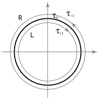
Figure 1: Contour $C$ surrounding the unit circle is shown together with our conventions in defining right and left fields.

The Poisson bracket for the fields $u_{0}(w)$ and $u_{1}(w)$ can be easily obtained from from (17,22) and (35) by analytic continuation. We find that $\left\{u_{0}(w),u_{0}(w^{\prime})\right\}=\left\{u_{1}(w),u_{1}(w^{\prime})\right\}=0$ and

$$\left\{u_{0}(w),u_{1}(w^{\prime})\right\} = ig\left(\frac{2\pi}{L}\right)^{2}\frac{ww^{\prime}}{(w-w^{\prime})^{2}}=ig\partial_{x}\frac{\pi}{L}\cot\frac{\pi}{L}(x-y).$$ (47)

5 Bilinearization and relation to MKP1 equation

The equations described in the previous section, their integrable structures and their connection to integrable hierarchies are the most transparent in bilinear form.

Let us introduce tau-functions $\tau_{0}$ and $\tau_{1}$ as

$$u_{0} = ig\partial_{x}\log\tau_{0},$$ (48)

$$u_{1} = -ig\partial_{x}\log\tau_{1}.$$

It can be easily checked that the 2BO (14) can be rewritten as an elegant bilinear Hirota equation on $\tau$-functions:

$$\left(iD_{t}+\frac{g}{2}\,D_{x}^{2}\right)\tau_{1}\cdot\tau_{0}=0.$$ (49)

Here we used the Hirota derivative symbols defined as

$$D_{x}^{n}f(x)\cdot g(x)\equiv\lim_{y\to x}(\partial_{x}-\partial_{y})^{n}f(x)g(y).$$ (50)

For example,

$$D_{t}f\cdot g = (\partial_{t}f)g-f(\partial_{t}g),$$

$$D_{x}^{2}f\cdot g = (\partial_{x}^{2}f)g-2(\partial_{x}f)(\partial_{x}g)+f(\partial_{x}^{2}g),$$ (51)

etc.

We emphasize that the bilinear equation holds on both sides of the unit circle. Introducing notations

$$\tau_{\pm 1}=\tau_{1}(x\pm i0)$$ (52)

we can rewrite the equation as

$$\left(iD_{t}+\frac{g}{2}\,D_{x}^{2}\right)\tau_{+1}\cdot\tau_{0}=0,$$ (53)

$$\left(iD_{t}+\frac{g}{2}\,D_{x}^{2}\right)\tau_{-1}\cdot\tau_{0=}\left(-iD_{t}+\frac{g}{2}\,D_{x}^{2}\right)\tau_{0}\cdot\tau_{-1}=0.$$ (54)

Equation (49) is the modified Kadomtsev-Petviashvili equation (MKP1). MKP1 contains two independent functions $\tau_{1}$ and $\tau_{0}$ and is formally not closed. The analyticity and reality conditions (29-32) stemming from the fact that all solutions are determined by two real functions $\rho(x,t)$ and $v(x,t)$, close the equation. Under these conditions the equations can be seen as a real reduction of MKP1. Let us formulate these conditions in terms of tau-functions.

The first requirement is that $\tau_{\pm 1}$ is analytic and does not have zeros for $\mbox{Im}\,x>0$ ($<0$) after analytic continuation. Also $\tau_{0}$ should be analytic and should not have zeros in the vicinity of the real axis, i.e., for $|\mbox{Im}\,x|<\epsilon$ for some $\epsilon>0$.

The second requirement is that $\tau_{\pm 1}$ should be related by Schwarz reflection (10). In terms of tau-functions it becomes on the unit circle (for real $x$)

$$\tau_{-1}=\overline{\tau_{+1}}e^{i\Theta(t)},$$ (55)

where a phase $\Theta(t)$ can be any time-dependent function.

The third requirement is related to the fact that $\mbox{Im}\,u_{0}$ is a function of density only and, therefore, can be expressed in terms of $u_{1}$ as can be easily seen from (17,22). This condition (32) can be written in a bilinear form as follows

$$iD_{x}\tau_{+1}\cdot{\tau_{-1}}=2\pi\,\tau_{0}\overline{\tau_{0}}.$$ (56)

The multiplicative constant in the r.h.s of (56) fixes the relative normalization of $\tau_{0}$ and $\tau_{1}$ and is arbitrary. We have chosen it to be $2\pi$.

Finally, we note that the pole ansatz solution (8,9) corresponds to the polynomial form of tau-functions with zeros at $w_{j}$ and $u_{j}$

$$\tau_{1}(w,t) = w^{-N/2}\prod_{j=1}^{N}(w-w_{j}(t)),$$ (57)

$$\tau_{0}(w,t) = w^{-N/2}\prod_{j=1}^{N}(w-u_{j}(t)).$$ (58)

6 Chiral Fields and Chiral Reduction

6.1 Chiral fields and currents

The 2BO equation can be conveniently expressed through yet another right and left handed chiral fields

$$J_{R,L}=v\pm g\left[\pi\rho+\partial_{x}(\log\sqrt{\rho})^{H}\right].$$ (59)

These fields are real. In terms of them, the 2BO equation (14) reads

$$\partial_{t}J_{R,L} + \partial_{x}\left(\frac{J_{R,L}^{2}}{2}\pm\frac{g}{2}\partial_{x}J_{R,L}^{H}\right)$$ (60)

$$\mp g\partial_{x}\left[J_{R,L}\partial_{x}(\log\sqrt{\rho})^{H}-(J_{R,L}\partial_{x}\log\sqrt{\rho})^{H}\right]=0.$$

Here $\rho$ is a function of $J_{R}$ and $J_{L}$ implicitly given by (59). The Hamiltonian acquires a Sugawara-like form

$$H=\frac{1}{8}\int dx\,\rho\Big{[}(J_{R}+J_{L})^{2}+(J_{R}^{H}-J_{L}^{H})^{2}\Big{]}$$ (61)

with Poisson brackets

$$\{J_{R,L}(x),J_{R,L}(y)\} = \pm 2\pi g\partial_{x}\delta(x-y)$$

$$\pm\frac{g}{2L}\partial_{x}\partial_{y}\left[\left(\frac{1}{\rho(x)}+\frac{1}{\rho(y)}\right)\cot\frac{\pi}{L}(x-y)\right],$$

$$\{J_{R}(x),J_{L}(y)\} = -\frac{g}{2L}\partial_{x}\partial_{y}\left[\left(\frac{1}{\rho(x)}-\frac{1}{\rho(y)}\right)\cot\frac{\pi}{L}(x-y)\right].$$ (63)

We note that Poisson brackets become canonical and left and right fields decouple in the limit of a constant density.

6.2 Chiral Reduction

We first note that the right and left currents $J_{R,L}$ are not separated in eq. (60). The equations for $J_{R}$ and $J_{L}$ are coupled through the density $\rho$ which should be found in terms of $J_{R,L}$ from (59). However, it is possible to find the chiral reductions of 2BO assuming that one of the currents is constant. We explain this reduction in some detail in this section.

The 2BO (14) or (60) admits an additional reduction to a chiral sector [15] where one of the chiral currents (59), say left current, is a constant $J_{L}(x,t)=v_{0}-\pi g\rho_{0}$. We can always choose a coordinate system moving with velocity $v_{0}$. This is equivalent to setting the zero mode of velocity to zero $v_{0}=0$. The condition $J_{L}=-\pi g\rho_{0}$ becomes

$$v=g\left[\pi(\rho-\rho_{0})+\partial_{x}(\log\sqrt{\rho})^{H}\right].$$ (64)

Then the currents can be expressed in terms of the density field only

$$J_{L}(x) = J_{0},$$

$$J_{R}(x) = J_{0}+J(x),$$ (65)

$$J_{0} = \pi g\rho_{0},$$

$$J(x) = 2g\left[\pi\left(\rho-\rho_{0}\right)+\partial_{x}(\log\sqrt{\rho})^{H}\right].$$ (66)

It follows from Eq. (60) that once the current $J_{L}$ is chosen to be constant $J_{L}(x)=J_{0}$ at $t=0$ it remains constant at any later time. The condition (64), therefore, is compatible with 2BO. Then the density $\rho(x,t)$ evolves according to the continuity equation (19) with velocity determined by the density according to (64). We obtain an important equation (written in the coordinate system moving with velocity $v_{0}$)

$$\rho_{t}+g\left[\rho\left(\pi\left(\rho-\rho_{0}\right)+\partial_{x}(\log\sqrt{\rho})^{H}\right)\right]_{x}=0.$$ (67)

We refer to this equation as the Non-Linear Chiral Equation (NLC). A substitution of the chiral constraint (65) to (61) gives the Hamiltonian for NLC

$$H = \frac{1}{8}\int dx\,\rho\left[J^{2}+(J^{H})^{2}\right]$$ (68)

with Poisson brackets for $J(x)$ following from (6.1). This equation constitutes one of major results of this paper.

NLC can be written in several useful forms. One of them is:

$$\varphi_{t}+g\left[\pi\rho_{0}\left(2e^{\varphi}-\varphi\right)+\frac{1}{2}\varphi_{x}^{H}\right]_{x}+\frac{g}{2}\varphi_{x}\varphi^{H}_{x}=0,$$ (69)

where $\rho(x)=\rho_{0}\,e^{\varphi(x)}$.

6.3 Holomorphic Chiral field

Under the chiral condition (64) the field $u_{0}$ becomes analytic inside the disk. Indeed, combining (64) and (22) we obtain

$$u_{0}(w)=\frac{1}{2}\oint\frac{d\zeta}{2\pi i\zeta}\,\frac{\zeta+w}{\zeta-w}J(\zeta),\quad|w|<1.$$ (70)

In the chiral case it has only non-negative powers of $w$ in the expansion (34). Negative modes vanish $b_{n}=0$. Conversely, the condition of $u_{0}$ to be analytic inside the unit disk is equivalent to $J_{L}=const$.

The current itself (65) is the boundary value of the field $\mbox{Re}\,u_{0}$ harmonic inside the disk

$$J(x)=2J_{0}+2\mbox{Re}\,u_{0}=2J_{0}+\sum_{n=1^{\infty}}\left(a_{n}w^{n}+\bar{a}_{n}w^{-n}\right).$$ (71)

The fields $u$ and $\tilde{u}$ are in turn also analytic inside the disk. Let $\varphi$ to be a harmonic function inside the disk with the boundary value $\log(\rho/\rho_{0})$. Then $\varphi=\phi(w)+\overline{\phi(w)}$, where $\phi(w)=(\log(\rho/\rho_{0}))^{+}$. Here $f^{+}(w)=\frac{1}{2}\int\frac{\zeta+w}{\zeta-w}f(\zeta)\,\frac{d\zeta}{2\pi i\zeta}$ is a function analytic in the interior of a unit circle which value on the boundary of the disk is $(f(x)-if^{H}(x))/2$. It follows from (24,64) that

$$u=-J_{0}+ig\partial\phi,\quad|w|<1,$$ (72)

$$\tilde{u}=u+4\pi g\rho_{0}\left(e^{\varphi}\right)^{+},\quad|w|<1,$$ (73)

Then 2BO (27) becomes an equation on an analytic function in the interior of a unit circle

$$\dot{\phi}+i\frac{g}{2}\left[(\partial\phi)^{2}+\partial^{2}\phi\right]+\pi g\rho_{0}\partial\left(2e^{\varphi}-\varphi\right)^{+}=0.$$ (74)

This is the “positive part” of (69) which is a direct consequence of (67).

We remark here that the chiral equation (67) has a geometric interpretation as an evolution equation describing the dynamics of a contour on a plane. Within this interpretation the term $\partial_{x}(\log\sqrt{\rho})^{H}$ of (67) is the curvature of the contour (see C).

6.4 Benjamin-Ono Equation

Another form of the Chiral Equation (67) arises when one considers the fields $u$ and $\tilde{u}$ outside the disk. There neither $u$ nor $\tilde{u}$ are analytic, but their boundary values are connected by the Hilbert transform

$$u(x-i0) = -J_{0}+2g\left[\pi\rho+i\partial_{x}(\log\sqrt{\rho})^{+}\right],$$ (75)

$$\tilde{u}(x-i0) = -J_{0}-iu^{H}(x-i0).$$ (76)

The bidirectional equation Eq. (27) complemented by this condition becomes unidirectional (chiral)

$$u_{t}+\partial_{x}\left[\frac{1}{2}u^{2}+\frac{g}{2}\partial_{x}u^{H}\right]=0.$$ (77)

This is just another form of the chiral equation (67).

The chiral equation (77) has the form of the Benjamin-Ono equation [13]. There are noticeable differences, however. Contrary to the Benjamin-Ono equation, Eq. (77) is written on a complex function, whose real and imaginary values at real $x$ are related by conditions (75) implementing the reality of the density:

$$\mbox{Re}\,u=-J_{0}+2g\pi\rho+g\left(\partial_{x}\log\sqrt{\rho}\right)^{H},\quad\mbox{Im}\,u=g\partial_{x}\log\sqrt{\rho}.$$ (78)

One understands this relation as a condition on the initial data. Once it is imposed by choosing the initial data for the density $\rho$, the condition remains intact during the evolution.

However, in the case when the deviation of a density is small with respect to the average density $|\rho-\rho_{0}|\ll\rho_{0}$, the imaginary part of $u$ vanishes in the leading order of $1/\rho_{0}$ expansion

$$u\approx J_{0}+2\pi g\varphi\approx 2\pi g(\rho-\rho_{0})+J_{0}$$

and the condition (78) becomes non-restrictive. In this limit Eq. (77) becomes an equation on a single real function. It is the conventional Benjamin-Ono equation. One can think of NLC (67) as of finite amplitude extension of BO. Similarly, 2BO is an integrable bidirectional finite amplitude extension of BO. It is interesting that there exists another bidirectional finite amplitude extension of BO – the Choi-Camassa equation [16]. However, it seems that the latter is not integrable.

7 Multi-phase solution

In this section we describe the most general finite dimensional solutions of 2BO. These are multi-phase solutions and their degenerations – multi-soliton solutions. In the former case the $\tau$-functions are polynomials of $e^{ik_{i}x}$, where $k_{i}$ is a finite set of parameters, the latter are just polynomials of $x$. These solutions are given by determinants of finite dimensional matrices. They appeared in the arXiv version of Ref. [17]. One can construct those solutions using the transformation (41) of 2BO to INLS (40). For the latter multi-phase solutions were written in [14] (see also [18, 19]). We use a different route in this section deriving multi-phase and multi-soliton solutions as a real reduction of corresponding solutions for MKP1.

7.1 Multi-phase and multi-soliton solutions of MKP1

We start from a general multi-phase solution of MKP1 equation and then restrict it to 2BO equation.

A general multi-phase solution of MKP1 equation

$$\left(iD_{t}+\frac{g}{2}\,D_{x}^{2}\right)\tau_{1}\cdot\tau_{0}=0.$$ (79)

is given by the following determinant formulae [21, 22]

$$\tau_{a} = e^{i\theta_{a}}\det\left[\delta_{jk}+c_{a,j}\frac{e^{i\theta_{j}}}{p_{j}-q_{k}}\right],\quad a=0,1$$ (80)

$$\frac{c_{1,j}}{c_{0,j}} = \frac{q_{j}-K-v_{0}}{p_{j}-K-v_{0}},$$ (81)

where the phases are

$$g\,\theta_{j}(x,t) = (q_{j}-p_{j})(x-x_{0j})-\frac{q_{j}^{2}-p_{j}^{2}}{2}t,$$ (82)

$$g\,\theta_{0}(x,t) = Kx-\frac{K^{2}}{2}t-\left((v_{0}+K)x-\frac{(v_{0}+K)^{2}}{2}t\right),$$ (83)

$$g\,\theta_{1}(x,t) = Kx-\frac{K^{2}}{2}t.$$ (84)

This solution is characterized by an integer number $N$ (number of “phases”), and by $4N-1$ parameters $p_{j}$, $q_{j}$, $c_{0,j}$, $x_{0j}$ and moduli $K$ and $v_{0}$. The solutions become single-valued on a unit circle if $p_{j}$ and $q_{j}$ are integers in units of $g\frac{2\pi}{L}$.

7.2 Multi-phase solution of 2BO

Without further restrictions the parameters entering (80-84) are general complex numbers. Reality nature of 2BO equation restricts them to be real.

The real moduli $K$ and $v_{0}$ are obviously zero modes of the fields $u_{1}$ and $u_{0}$ respectively, and therefore, they are zero modes of the density $\rho_{0}=\frac{1}{L}\int\rho\,dx=-K/(\pi g)$ and velocity $\frac{1}{L}\int v\,dx=v_{0}$.

7.2.1 Schwarz reflection condition

We have to restrict the coefficients $c_{a,j}$, so that there exists another solution $\tau_{-1},\tau_{0}$ of Eq. (79) sharing the same $\tau_{0}$ with the solution (86,87) and obeying the Schwarz reflection property (55).

The Galilean symmetry of the equation (79) is here to help. If $\tau_{a}(x,t),\,a=0,1$ give a solution of (79) then the pair $e^{iP_{a}x-iE_{a}t}\tau_{a}(x-gP_{a}t,t)$ is also a solution provided that $E_{a+1}-E_{a}=\frac{1}{2}(P_{a+1}-P_{a})^{2}$.

Being applied to the solution (80-84) the Galilean invariance can be utilized as follows. We notice from (82) that

$$\theta_{j}(x-Pt,t;\left\{p_{j},q_{j}\right\})=\theta_{j}(x,t;\left\{p_{j}+P,q_{j}+P\right\}).$$ (85)

Performing the Galilean boost to (80), multiplying both tau-functions by $e^{-iPv_{0}t}$ and shifting $p_{j}\to p_{j}-P$, $q_{j}\to q_{j}-P$ we obtain that

$$\tau_{-1} = e^{i\theta_{1}-iP(K+v_{0})t+\frac{i}{g}(Px-\frac{P^{2}}{2}t)}\det\left[\delta_{jk}+b_{j}\frac{e^{i\theta_{j}}}{p_{j}-q_{k}}\right],$$ (86)

$$\frac{b_{j}}{c_{0,j}} = \frac{q_{j}-K-v_{0}-P}{p_{j}-K-v_{0}-P}$$ (87)

form a solution of (79) with the same $\tau_{0}$ (80).

Now we are going to show that for a particular choice of coefficients $c_{1,j}$ the Galilean boosted solution (86,87) is a complex conjugate of $\tau_{+1}$ from (80). To show this we will employ the determinant identity (143).

We apply the determinant identity (143) to (86) and obtain

$${\tau}_{-1} = e^{i\theta_{1}-iP(K+v_{0})t+\frac{i}{g}(Px-\frac{P^{2}}{2}t)}\left(\prod_{j}e^{i\theta_{j}}\sqrt{\frac{b_{j}}{\tilde{b}_{j}}}\right)\det\left[\delta_{jk}+\tilde{b}_{j}\frac{e^{-i\theta_{j}}}{p_{j}-q_{k}}\right],$$ (88)

where

$$\tilde{b}_{j}b_{j}=(p_{j}-q_{j})^{2}{\prod_{k\neq j}}\frac{(p_{j}-q_{k})(q_{j}-p_{k})}{(p_{j}-p_{k})(q_{j}-q_{k})}.$$ (89)

The Schwarz reflection condition(55) ${\tau}_{-1}=\overline{\tau_{+1}}e^{i\Theta(t)}$ requires

$$\tilde{b}_{j}=c_{1,j},$$ (90)

determines $\Theta(t)$, and gives a relation

$$P=\sum_{j}(p_{j}-q_{j})-2K.$$ (91)

Finally, combining all relations (81,87,89,90) together we obtain the condition on coefficients $c_{a,j}$

$$\left(\frac{c_{a,j}}{p_{j}-q_{j}}\right)^{2} {\prod_{k\neq j}}\frac{(p_{j}-p_{k})(q_{j}-q_{k})}{(p_{j}-q_{k})(q_{j}-p_{k})}$$

$$= \left(\frac{p_{j}-K-v_{0}}{q_{j}-K-v_{0}}\right)^{1-2a}\frac{p_{j}-K-v_{0}-P}{q_{j}-K-v_{0}-P}.$$

Condition (7.2.1) is necessary to turn a general solution of MKP1 into a solution of 2BO. We also have to find a condition that guarantees that $\tau_{1}$ has no zeros inside the unit disk. Before turning to this analysis, we first discuss degeneration of formulas (80) into multi-soliton solution.

7.2.2 Multi-soliton solution of 2BO

The multi-soliton solution of 2BO follows from the multi-phase solution in the limit $p_{j}\to q_{j}$. We introduce

$$k_{j} = p_{j}-q_{j},$$ (93)

$$v_{j} = \frac{1}{2}(p_{j}+q_{j})$$ (94)

and consider the limit $k_{j}\to 0$ keeping $v_{j}$ fixed. After some straightforward calculations we obtain

$$\tau_{a} = e^{i\theta_{a}}\det\left[\delta_{jk}\left(x-x_{0j}-v_{j}t+iA_{a,j}\right)+ig\frac{1-\delta_{jk}}{v_{j}-v_{k}}\right],$$ (95)

$$A_{a,j} = \frac{g}{2}\left(\frac{1}{v_{j}-v_{0}+K}\pm\frac{1}{v_{j}-v_{0}-K}\right),\quad a=0,1.$$ (96)

One notices that in the limit $t\to+\infty$ the solution (95) asymptotically goes to the factorized form

$$\tau_{a}\to e^{i\theta_{a}}\prod_{j}(x-x_{0j}-v_{j}t+iA_{a,j}),$$ (97)

describing separated single solitons.

Eq. (97) gives a large time value of zeros of $\tau_{1}$. Their imaginary part is

$$-\mbox{Re}\,A_{1,j}=g\frac{K}{(v_{j}-v_{0})^{2}-K^{2}}.$$ (98)

It must be negative in order for $\tau_{1}$ to have no zeroes inside the unit disk. Since $K<0$ we must require

$$(v_{j}-v_{0})^{2}>K^{2}.$$ (99)

In the next paragraph we argue that under this condition and additional restrictions on parameters $p_{j}$, $q_{j}$ (see eq. (109) below) the moving zeros never cross the real axis, and therefore zeros stay outside of the unit disk at all times.

To conclude this section we note a unique property of the 2BO equation (shared with the BO equation). Namely, there is a “quantization” of the mass of solitons: each soliton of 2BO carries a unit of mass regardless of its velocity. We have for $N$-soliton solution

$$\int dx\,(\rho-\rho_{0})=N.$$ (100)

Where $K=-\pi g\rho_{0}$. The total momentum, and the total energy of a multisoliton solution is given by

$$\int dx\,(\rho v-\rho_{0}v_{0})=\sum_{j}v_{j},$$ (101)

$$\int dx\,\left(\frac{\rho v^{2}}{2}+\rho\epsilon(\rho)-\frac{\rho_{0}v_{0}^{2}}{2}-\rho_{0}\epsilon(\rho_{0})\right)=\sum_{j}\frac{v_{j}^{2}}{2},$$ (102)

where $\epsilon(\rho)$ is defined in (37).

One-soliton solution has a form

$$\rho = \rho_{0}+\frac{1}{\pi}\frac{A_{1}}{(x-x_{01}-v_{1}t)^{2}+A_{1}^{2}},$$ (103)

$$v = v_{0}+g\frac{A_{0}}{(x-x_{01}-v_{1}t)^{2}+A_{0}^{2}},$$ (104)

where

$$A_{1} = \mbox{Re}\,A_{1,1}=\frac{\pi g^{2}\rho_{0}}{(v_{j}-v_{0})^{2}-(\pi g\rho_{0})^{2}},$$ (105)

$$A_{0} = \mbox{Re}\,A_{0,1}=\frac{g(v_{j}-v_{0})}{(v_{j}-v_{0})^{2}-(\pi g\rho_{0})^{2}}.$$ (106)

This one-soliton solution has been found first in Ref. [7] (see also [23]).

7.2.3 Analyticity condition

Now we can turn to the multiphase solution and derive conditions sufficient in order for $u_{1}$ to be analytic in the upper half-plane in complex $x$-variable (inside the unit disk). Analyticity in the lower half-plane follows from the Schwarz reflection condition (55). We will follow the approach of Dobrokhotov and Krichever [24] developed for Benjamin-Ono equation.

Analyticity of $u_{1}$ means that $\tau_{1}$ given by (80) has no zeros in the upper half plane, or that the matrix

$$M_{jk}=\delta_{jk}+\frac{c_{1,j}e^{i\theta_{j}}}{p_{j}-q_{k}}$$ (107)

is non-degenerate. Following the approach of Ref. [24] we derived in E a sufficient condition of non-degeneracy of the matrix $M$ from (107). Let us now write that condition (153,152) with $c_{j}$ defined by (144,7.2.1). We obtain (calculating $f_{j}$)

$$\frac{P}{\tilde{p}_{j}(\tilde{q}_{j}-P)}\prod_{k(k\neq j)}\frac{\tilde{p}_{j}-\tilde{q}_{k}}{\tilde{p}_{j}-\tilde{p}_{k}}\;\;\mbox{same sign for all }j,$$ (108)

where we used shifted numbers $\tilde{p}_{j}=p_{j}-K-v_{0}$ and similar for $\tilde{q}_{j}$. Here $P=-2K+\sum_{j}(\tilde{p}_{j}-\tilde{q}_{j})$.

The set of conditions

$$\tilde{q}_{1}<\tilde{p}_{1}<\ldots<\tilde{q}_{m}<\tilde{p}_{m}<0<P<\tilde{q}_{m+1}<\tilde{p}_{m+1}<\ldots<\tilde{q}_{N}<\tilde{p}_{N}$$ (109)

satisfies (108). Moreover, (109) yields to (99), which in its turn means that at least at some values of parameters (large time and soliton limit) no zeros of $\tau_{1}$ are inside the unit disk. Since they also can not be on the circle they do not cross it while moving in time and in the space of parameters.

Condition (109) suggests that a general solution is characterized by a integer number $N-2m$. This is chirality – the difference between the number of $N-m$ right and $m$ - left moving modes

$$\frac{1}{2\pi g}\int(J_{R}-v_{0}-\pi g\rho_{0})\,dx = N-m,$$ (110)

$$\frac{1}{2\pi g}\int(J_{L}-v_{0}+\pi g\rho_{0})\,dx = m.$$ (111)

Eqs. (80-84,7.2.1,109) summarize a general finite dimensional quasi-periodic solution. We emphasize here that this solution is not chiral and contains both right and left-moving modes.

7.3 Multi-phase solution of the Chiral Non-linear Equation

The (right) chiral case appears when $\tau_{0}$ has no zeros outside the unit disk. It naturally happens when the number of, say, left-moving modes $m$ in (109) vanishes $m=0$. In this case all $v_{j}-v_{0}<0$. In their turn, imaginary parts of zeros of $\tau_{0}$ in the multi-soliton limit (as in (98))

$$-A_{0j}=-g\frac{v_{j}-v_{0}}{(v_{j}-v_{0})^{2}-K^{2}}>0$$ (112)

are positive. One can check that in this case (107) with $c_{1,j}\to c_{0,j}$ is non-degenerate for arbitrary values of parameters satisfying (109) with $m=0$ (and similarly for $m=N$). Therefore, $\tau_{0}(x)$ is non-zero in one of half-planes.

This is a chiral multi-phase solution of 2BO.

7.4 Multi-phase solution of the Benjamin-Ono equation

The known solutions of the Benjamin-Ono equation [20, 21] are obtained from the solutions of the Chiral Non-linear equation by taking the limit $\rho_{0}\to\infty$. In this case $K\to-\infty$ and conditions (109) allow for a good limit only if $m=N$ (left sector) or $m=0$ (right sector). Let us concentrate on the right sector. We redefine $p_{j}\to p_{j}-K$, $q_{j}\to q_{j}-K$, $v_{0}\to v_{0}-2K$, go to the frame moving with velocity $-K$ ($x\to x+Kt$), and obtain from (109,7.2.1) in the limit $K\to-\infty$

$$q_{1}<p_{1}<q_{2}<\ldots<q_{N}<p_{N},$$ (113)

$$\left(\frac{c_{a,j}}{p_{j}-q_{j}}\right)^{2}{\prod_{k\neq j}}\frac{(p_{j}-p_{k})(q_{j}-q_{k})}{(p_{j}-q_{k})(q_{j}-p_{k})}=\left(\frac{p_{j}-v_{0}}{q_{j}-v_{0}}\right)^{1-2a}$$ (114)

with solution given by (80,82) and with (83,84) (one should put $K=0$ in latter two). This is nothing else but the multiphase solution of conventional Benjamin-Ono equation [21, 18].

7.5 Moving Poles

The 2BO equation (14) looks very similar to the classical BO equation. One of important tools in studying the classical BO equation is the so-called pole ansatz - solutions in the form of poles moving in a complex plane. [20] We have already seen that the pole ansatz (8,9) describes the dynamics of the original Calogero-Sutherland model with finite number of particles $N$.

In this section we consider collective excitations of Calogero-Sutherland model in the limit of infinitely many particles. These excitations are given by “complex” pole solutions of the 2BO.

In the Pole Ansatz (8,9), the reality conditions were satisfied by requiring $x_{j}$ to be real (or $w_{j}(t)$ moving on a unit circle). One could generalize the Pole Ansatz (8,9) to case where $w_{j}(t)$ are away from the unit circle and moving in a complex plane. The equations (6,7) describing the motion of poles preserve their form. However, $u_{-1}(w)$ outside of the unit circle is not related to the $u_{1}(w)$ inside of the circle by analytic continuation but only by Schwarz reflection (10). The field $u_{1}(w)$ is analytic inside the unit circle and has moving poles outside of the unit circle (and vice versa for $u_{-1}(w)$). Of course, having obtained the solution of 2BO inside the unit circle does not mean automatically that the Schwarz reflected function (10) will solve 2BO in the exterior of the circle with the same $u_{0}$. The property (10) requires that (6,7) are satisfied not only by $u_{j}$ and $w_{j}$ but also by $u_{j}$ and $1/\bar{w}_{j}$. This requirement will significantly constrain the positions of poles $w_{j}$ and $u_{j}$ in a complex plane. It turns out that this constraint allows for non-trivial solutions.

We emphasize here once again that while real axis poles $x_{j}$ of $u_{1}$ in the pole ansatz represent the original CS particles, the complex poles $x_{j}$ represent collective excitations of the CS liquid moving in the background of macroscopic number of particles.

Instead of looking for moving pole solution in this section we have taken a different route. We first construct the much more general solution of 2BO (14) with proper reality conditions and then obtain a moving pole (i.e., multi-soliton) solution as a limit of the multi-phase solution. One can see from (95) that for soliton solutions the zeros of tau-functions move in a complex plane. It is especially clear at large times when solitons are well separated (97).

8 Conclusion and discussion

In this paper we have shown that the dynamics of the classical Calogero-Sutherland model in the limit of infinite number of particle is equivalent to the bidirectional Benjamin-Ono equation (14). The bidirectional Benjamin-Ono equation (2BO) is an integrable classical integro-differential equation. Its integrability can be deduced from the fact that it is a Hamiltonian reduction of MKP1 as it is shown in this paper. As an alternative, one can use the equivalence of 2BO to INLS (40). The integrability of INLS was proven and the spectral transform was constructed for INLS in Ref. [25] (see also [19]). Therefore, one can use all techniques developed in the field of classical integrable equations for 2BO. It has multi-phase solutions (explicitly constructed in this paper), bi-Hamiltonian structure, an associated hierarchy of higher order equations, etc. 2BO is intrinsically simpler than many other classical integrable models. Its solitons have “quantized” area independent of soliton’s velocity. The collision of two solitons goes without any time delay etc. This is a reflection of the fact that underlying Calogero-Sutherland model is essentially a model of non-interacting particles in disguise. In particular, 2BO supports a phenomenon of dispersive shock waves. Some applications of this phenomenon to quasi-classical description of quantum systems were considered in [15].

Most of the results of this paper can be generalized along two avenues: generalization to an elliptic case and generalization to a quantum model.

The Calogero-Sutherland model (trigonometric case) can be generalized to an elliptic case — elliptic Calogero model where the interaction between particles is either Weierstrass $\wp(x|\omega_{1},\omega_{2})$-function with purely real and purely imaginary periods $\omega_{1},i\omega_{2}$, and to its hyperbolic degeneration (hyperbolic case) with inter-particle interaction given by $\sinh^{-2}(x/\omega_{2})$ (see [3] for review).

In both cases most of formulas remain unchanged if one substitutes the Hilbert transform $f^{H}$ for a transform with respect to a strip $0<\mbox{Im}\,x<\omega$, where $\omega$ is an imaginary period

$$f^{H}=\int\zeta(x-x^{\prime})f(x^{\prime})dx^{\prime}\;\;\;\;\mbox{or}\;\;\;\int\frac{1}{\omega_{2}}\coth\frac{1}{\omega_{2}}(x-x^{\prime})f(x^{\prime})dx^{\prime}.$$ (115)

In the first case the integration goes over a real period of the Weierstrass $\zeta$-function.

The elliptic Calogero model allows one to study a crossover between liquids with long range inter-particle interaction to liquids with short range interaction. In the limit of a large imaginary period $\omega_{2}\to\infty$ the $\wp$-function degenerates to $1/\sin(x/\omega_{1})^{2}$ – the case of long range inter-particle interaction. The opposite limit $\omega_{2}\to 0$ gives rise to a short range interaction: $\omega_{2}\wp(x)\to\delta(x)$.

In the latter case the the Hilbert transform (115) becomes a derivative $f^{H}\to\omega\partial_{x}f$ and the equations discussed in this paper become local. In particular the Benjamin-Ono equation flows to the KdV equation, while the bidirectional BO-equation flows to NLS - the nonlinear Schrödinger equation.

2BO in the limit of small amplitudes and in the chiral sector becomes the conventional Benjamin-Ono equation. In elliptic case (and in the hyperbolic one) the limit of small amplitudes in the chiral sector leads to a generalization of the Benjamin-Ono equation, known as the ILW (Intermediate Long Wave) equation [8]. Contrary to the Benjamin-Ono equation and to 2BO, the latter and its bidirectional generalization 2ILW have elliptic solutions.

We intend to address the elliptic case in a separate publication.

Probably, even more interesting is a generalization of the results of this paper to the quantum case. It is well known that the classical CSM model (1) can be lifted to a quantum integrable Calogero-Sutherland model [1, 2, 27]. The latter model is defined by (1) with $g^{2}\to\hbar^{2}\lambda(\lambda-1)$ and $p_{i}=-i\hbar\partial_{x_{i}}$. The 2BO equation in the form (14) remains unchanged, except for the change of the coefficient $g\to\lambda-1$ and for the change of Poisson brackets (47) by a commutator: $\{\,,\,\}\to\frac{i}{\hbar}[\,,\,]$. The change $g\to\lambda-1$ valid for eq. (14) is not correct for all formulas. For example, the bilinear form of classical 2BO (49) is identical to its quantum version with just a change of notations $g\to\lambda$. For some details see [4]. Multi-soliton solution of 2BO presented here corresponds to exact quasiparticle excitations of quantum Calogero-Sutherland model [29, 7]. The more detailed study of the relations between integrable structures of the classical 2BO and its quantum analogue is necessary.

9 Acknowledgments

AGA is grateful to A. Polychronakos for the discussion of the chiral case. PW thanks J. Shiraishi for discussions. The work of AGA was supported by the NSF under the grant DMR-0348358. EB was supported by ISF grant number 206/07. PW was supported by NSF under the grant NSF DMR-0540811/FAS 5-27837 and MRSEC DMR-0213745. We also thank the Galileo Galilei Institute for Theoretical Physics for the hospitality and the INFN for partial support during the completion of this work.

Appendix A Hilbert transforms

Given a function $f(x)$, $f(x)\to 0$ as $x\to\pm\infty$, the Hilbert transform is defined as

$$f^{H}(x)=\frac{1}{\pi}\mathchoice{{\vbox{\hbox{$\textstyle-$}}\kern-4.86108pt}}{{\vbox{\hbox{$\scriptstyle-$}}\kern-3.25pt}}{{\vbox{\hbox{$\scriptscriptstyle-$}}\kern-2.29166pt}}{{\vbox{\hbox{$\scriptscriptstyle-$}}\kern-1.875pt}}\!\int_{-\infty}^{+\infty}dy\,\frac{f(y)}{y-x}.$$ (116)

For periodic functions with period $L$ we define the transform as

$$f^{H}(x)=\mathchoice{{\vbox{\hbox{$\textstyle-$}}\kern-4.86108pt}}{{\vbox{\hbox{$\scriptstyle-$}}\kern-3.25pt}}{{\vbox{\hbox{$\scriptscriptstyle-$}}\kern-2.29166pt}}{{\vbox{\hbox{$\scriptscriptstyle-$}}\kern-1.875pt}}\!\int_{0}^{L}\frac{dy}{L}\,f(y)\cot\frac{\pi}{L}(y-x).$$ (117)

The Hilbert transform of the constant function is zero. The Hilbert transform is inverse to itself $H^{2}=-1$ or $(f^{H})^{H}=-f$ and it commutes with derivative $(f^{H})_{x}=(f_{x})^{H}.$ More generally, a function $f(x)$ defined on the closed (directed) contour $C$ surrounded the origin of a complex plane can be decomposed into a sum $f=f^{+}+f^{-}$, analytic functions $f^{\pm}$ inside (outside) of the contour, such that $f^{+}(0)=f^{-}(\infty)$. Then

$$f^{H}\equiv P\oint\frac{d\zeta}{2\pi\zeta}\,f(\zeta)\frac{\zeta+w}{\zeta-w}=i(f^{+}-f^{-}).$$ (118)

Using (118) it is easy to derive the following properties:

$$f^{H}g+fg^{H} = (fg)^{H}-(f^{H}g^{H})^{H}$$ (119)

and some integration formulas

$$\int dx\,f^{H} = 0,$$ (120)

$$\int dx\,f^{H}g = -\int dx\,fg^{H},$$ (121)

$$\int dx\,f^{H}f = 0.$$ (122)

From (118) we have for functions analytic in one of half planes

$$(f^{\pm})^{H}=\pm if^{\pm}$$ (123)

and as an immediate consequence

$$(e^{ikx})^{H} = ie^{ikx}\,\mbox{sgn}\,k,$$ (124)

$$\left(\frac{1}{x-a}\right)^{H} = \frac{i}{x-a}\;\;\;\;\mbox{for}\;\mbox{Im}\,a>0.$$ (125)

Generally, in Fourier space the Hilbert transform is equivalent to a multiplication by $i\,\mbox{sgn}\,k$, i.e., for Fourier coefficients

$$(f^{H})_{k}=i(\,\mbox{sgn}\,k)f_{k}.$$ (126)

It is easy to derive the following useful identities

$$\int u^{2}\,dx = \int(u^{H})^{2}\,dx,$$ (127)

$$\int u^{3}\,dx = 3\int u(u^{H})^{2}\,dx,$$ (128)

$$\int u^{4}\,dx = \int\left[(u^{H})^{4}+6u^{2}(u^{H})^{2}\right]\,dx,$$ (129)

$$\int u^{5}\,dx = 5\int\left[u(u^{H})^{4}-2u^{3}(u^{H})^{2}\right]\,dx.$$ (130)

Appendix B Conserved integrals of 2BO

In this section we present the conserved integrals of 2BO written in different forms. The contour integrals below are taken along the contour $C$ defined in Figure 1.

$$I_{1} = \oint\frac{dx}{2\pi g}\,u=\int dx\,\rho=\int\frac{dx}{2\pi}\,i\partial_{x}\log\frac{\tau_{1}}{\tau_{-1}},$$ (131)

$$I_{2} = \oint\frac{dx}{2\pi g}\,\frac{1}{2}u^{2}=\oint\frac{dx}{2\pi g}\,u_{1}u_{0}=\int dx\,\rho v$$ (132)

$$= \frac{g}{2}\int\frac{dx}{2\pi}\,\left[\frac{D_{x}^{2}\tau_{-1}\cdot\tau_{0}}{\tau_{-1}\tau_{0}}-\frac{D_{x}^{2}\tau_{1}\cdot\tau_{0}}{\tau_{1}\tau_{0}}\right]=i\partial_{t}\int\frac{dx}{2\pi}\,\log\frac{\tau_{1}}{\tau_{-1}},$$

$$I_{3} = \oint\frac{dx}{2\pi g}\,\left[\frac{1}{3}u^{3}+i\frac{g}{2}u\partial_{x}\tilde{u}\right]$$ (133)

$$= \oint\frac{dx}{2\pi g}\,\left[{u_{1}}^{2}u_{0}+u_{1}{u_{0}}^{2}+igu_{1}\partial u_{0}\right]=\int dx\,\left[\frac{\rho v^{2}}{2}+\rho\epsilon(\rho)\right].$$

Higher integrals of motion for 2BO can be constructed recurrently similarly to Benjamin-Ono equation [26] or can be written using the integrals obtained for INLS [25, 19].

Appendix C Geometrical interpretation of the chiral equation: Contour dynamics

Equation (67) can be cast in the form of contour dynamics.

Let us interpret the unit disk as a uniformization of a simply-connected domain embedded into the complex $z$-plane. In other words, $z(w)$ is a conformal map of the interior of the unit disk $|w|=1$ to a bounded domain such that the length element of its boundary is proportional to the density

$$ds\equiv|z^{\prime}(x)|dx=\pi\rho(x)dx.$$ (134)

(equivalently $1/\sqrt{\rho}$ is a harmonic measure of the contour). Then the equation (67) describes the evolution of the planar domain. We notice that the curvature of the boundary $\kappa=-i\partial_{s}\log z_{s}$ can be expressed in terms of the density $\rho(x)$ as

$$\kappa=-(\pi\rho)^{-1}\left(\partial_{x}\left(\log\sqrt{\rho}\right)^{H}-1\right).$$ (135)

Then (67) can be written as

$$\frac{ds}{dt}=g\left(\frac{ds}{dx}\right)^{2}(1-\kappa),$$ (136)

where ${d}/{dt}=\partial_{t}-g\pi\rho_{0}\,\partial_{x}$ and the time derivative is taken at fixed $x$. The equation (136) describes the evolution of a planar contour driven by its curvature.

Appendix D Determinant identity

Here we present a derivation of a determinant identity (143) which was used in Sec. 7.2.

Consider the Cauchy matrix

$$D_{ij}=\frac{r_{i}s_{j}}{p_{i}-q_{j}},\quad p_{i}\neq q_{j},\qquad i,j=1,2,\ldots,N.$$ (137)

Its determinant

$$\det(D)=\prod_{i}r_{i}\frac{\prod_{i<j}(p_{i}-p_{j})(q_{j}-q_{i})}{\prod_{i,j}(x_{i}-y_{j})}\prod_{j}s_{j}=\left(\prod_{i}r_{i}s_{i}\tilde{r}_{i}\tilde{s}_{i}\right)^{-\frac{1}{2}},$$ (138)

where $\tilde{r}_{i}$ and $\tilde{s}_{i}$ are defined by

$$\tilde{r}_{i}r_{i} = (p_{i}-q_{i}){\prod_{k(k\neq i)}}\frac{p_{i}-q_{k}}{p_{i}-p_{k}},$$ (139)

$$\tilde{s}_{i}s_{i} = -(q_{i}-p_{i}){\prod_{k(k\neq i)}}\frac{q_{i}-p_{k}}{q_{i}-q_{k}}.$$ (140)

The inverse of $D$ is also Cauchy matrix (see e.g., [28]) given by

$$(D^{-1})_{ij}=\frac{\tilde{r}_{j}\tilde{s}_{i}}{p_{j}-q_{i}}.$$ (141)

The obvious identity

$$\det(1+D)=\det(D)\det(1+(D^{T})^{-1})$$ (142)

being specialized for Cauchy matrix $D$ (137) reads

$$\frac{\det\Big{(}\delta_{ij}+\frac{r_{i}s_{j}}{p_{i}-q_{j}}\Big{)}}{\left(\prod_{i}r_{i}s_{i}\right)^{1/2}}=\frac{\det\Big{(}\delta_{ij}+\frac{\tilde{r}_{i}\tilde{s}_{j}}{p_{i}-q_{j}}\Big{)}}{\left(\prod_{i}\tilde{r}_{i}\tilde{s}_{i}\right)^{1/2}}.$$ (143)

Appendix E Non-degeneracy condition of matrix (107)

In this section we will derive the non-degeneracy condition for the matrix (107) following [24].

Let us introduce

$$c_{j}=c_{1,j}\exp\left\{\frac{i}{g}\left[(q_{j}-p_{j})x-\frac{q_{j}^{2}-p_{j}^{2}}{2}t\right]\right\}.$$ (144)

Our aim is to derive a sufficient condition on coefficients $c_{j}$ for the matrix

$$M_{jk}=\delta_{jk}+\frac{c_{j}}{p_{j}-q_{k}}$$ (145)

to be non-degenerate for real $p_{j}$ and $q_{j}$.

Let us assume that the matrix (145) is degenerate. It means the the following equation has a non-zero solution

$$r_{j}+\sum_{k}\frac{c_{j}}{p_{j}-q_{k}}r_{k}=0.$$ (146)

We introduce the meromorphic function

$$\psi(z)=\sum_{k}\frac{r_{k}}{z-q_{k}}$$ (147)

and rewrite the condition (146) as

$$r_{j}=\mbox{\rm res}_{z=q_{j}}\psi(z)=-c_{j}\psi(p_{j}).$$ (148)

Now, let us consider the function

$$f(z)=\psi(z)\overline{\psi(\bar{z})}\prod_{j}\frac{z-q_{j}}{z-p_{j}}.$$ (149)

Here explicitly

$$\overline{\psi(\bar{z})}=\sum_{k}\frac{\bar{r}_{k}}{z-q_{k}}.$$ (150)

The function $f(z)$ is meromorphic and its residue at infinity is zero (as $\psi(z)\sim z^{-1}$ as $z\to\infty$). On the other hand ($p_{j}$ and $q_{j}$ are real numbers)

$$\mbox{\rm res}_{z=p_{j}}f+\mbox{\rm res}_{z=q_{j}}f=\psi(p_{j})\overline{\psi(p_{j})}(p_{j}-q_{j})\prod_{k(k\neq j)}\frac{p_{j}-q_{k}}{p_{j}-p_{k}}$$

$$+r_{j}\bar{r}_{j}\frac{1}{q_{j}-p_{j}}\prod_{k(k\neq j)}\frac{q_{j}-q_{k}}{q_{j}-p_{k}}=\frac{|r_{j}|^{2}}{|c_{j}|^{2}}\,f_{j},$$ (151)

where we introduced a notation

$$f_{j}=(p_{j}-q_{j})\prod_{k(k\neq j)}\frac{p_{j}-q_{k}}{p_{j}-p_{k}}\left[1-\frac{|c_{j}|^{2}}{(p_{j}-q_{j})^{2}}\prod_{k(k\neq j)}\frac{(p_{j}-p_{k})(q_{j}-q_{k})}{(p_{j}-q_{k})(q_{j}-p_{k})}\right].$$ (152)

If $f_{j}$ has the same sign for all $j$, e.g., $f_{j}<0$ we immediately obtain

$$\sum_{j}\left(\mbox{\rm res}_{z=p_{j}}f+\mbox{\rm res}_{z=q_{j}}f\right)<0.$$

This is impossible as the residue of $f(z)$ at infinity is zero. This contradiction shows that the matrix (145) is nondegenerate under these conditions.

To summarize, the sufficient condition of non-degeneracy of (145) is

$$f_{j}<0\;\;\mbox{for all }j\qquad\qquad\mbox{or }\qquad\qquad f_{j}>0\;\;\mbox{for all }j,$$ (153)

where $f_{j}$ are defined according to (152).

References

References

• [1] F. Calogero, J. Math. Phys. 10, 2191, 2197 (1969); 12, 419 (1971).
• [2] B. Sutherland, Phys. Rev. A 4, 2019 (1971); A 5, 1372 (1972). Phys. Rev. Lett. 34, 1083 (1975).
• [3] M. A. Olshanetsky and A. M. Perelomov, Phys. Rep. 71, pp. 313-400, (1981).
Classical integrable finite-dimensional systems related to Lie algebras.
• [4] A. G. Abanov and P. B. Wiegmann, Phys. Rev. Lett 95, 076402 (2005).
Quantum Hydrodynamics, the Quantum Benjamin-Ono equation, and the Calogero Model.
• [5] I. Andrić, A. Jevicki, and H. Levine, Nucl. Phys. B215, 307 (1983).
On the large-N limit in symplectic matrix models.
• [6] I. Andrić and V. Bardek, J. Phys. A 21, 2847 (1988).
1/N corrections in Calogero-type models using the collective-field method.
ibid. 24, 353 (1991).
Collective-field method for a U(N)-invariant model in the large-N limit.
• [7] A. P. Polychronakos, Phys. Rev. Lett. 74, 5153 (1995).
Waves and Solitons in the Continuum Limit of the Calogero-Sutherland Model.
• [8] M. A. Ablowitz and P. A. Clarkson, Solitons, Nonlinear Evolution Equations and Inverse Scattering, London Math. Society Lecture Note Series (No. 149), 1991.
• [9] H. Awata, Y. Matsuo, S. Odake, J. Shiraishi, Phys. Lett. B 347, 49-55, (1995).
Collective field theory, Calogero-Sutherland model and generalized matrix models.
• [10] A. Jevicki and B. Sakita, Nucl. Phys. B165, 511 (1980).
The Quantum Collective Field Method and its Application to the Planar Limit.
• [11] B. Sakita, Quantum Theory of Many-variable Systems and Fields. World Scientific, 1985.
• [12] A. Jevicki, Nucl. Phys. B376, 75-98 (1992).
Nonperturbative Collective Field Theory.
• [13] T. B. Benjamin, J. Fluid Mech. 29, 559 (1967).
Internal waves of permanent form in fluids of great depth.
H. Ono, J. Phys. Soc. Japan 39, 1082 (1975).
Algebraic solitary waves in stratified fluids.
• [14] D. Pelinovsky, Phys. Lett. A 197, 401-406 (1995).
Intermediate nonlinear Schrödinger equation for internal waves in a fluid of finite depth.
• [15] E. Bettelheim, A. G. Abanov, and P. Wiegmann, Phys. Rev. Lett. 97, 246401 (2006).
Nonlinear quantum shock waves in fractional quantum hall edge states.
• [16] W. Choi and R. Camassa, Phys. Rev. Lett. 77, 1759-1762 (1996).
Long internal waves of finite amplitude.
• [17] E. Bettelheim, A. G. Abanov, and P. Wiegmann, appendix of arXiv:cond-mat/0606778 (2006), unpublished.
Quantum Shock Waves - the case for non-linear effects in dynamics of electronic liquids.
• [18] Y. Matsuno, J. Phys. Soc. Jap., 73, 3285-3293 (2004).
New Representations of Multiperiodic and Multi-soliton Solutions for a Class of Nonlocal Soliton Equations.
• [19] Y. Matsuno, Inv. Probl. 20, 437-445 (2004).
A Cauchy problem for the nonlocal nonlinear Schrödinger equation.
• [20] H. H. Chen, Y. C. Lee, and N. R. Pereira, J. Phys. Fluids 22, 187 (1979).
Algebraic internal wave solitons and the integrable Calogero-Moser-Sutherland $N$-body problem.
• [21] J. Satsuma and Y. Ishimori, J. Phys. Soc. Jpn., 46, pp. 681-687 (1979).
Periodic Wave and Rational Soliton Solutions of the Benjamin-Ono Equation.
• [22] Y. Matsuno, Bilinear Transformation Method, in v. 174, Math. in science and engineering, Academic Press, 1984.
• [23] I. Andrić, V. Bardek, L. Jonke, Phys. Lett. B 357, 374 (1995).
Solitons in the Calogero-Sutherland collective-field model.
• [24] S. Yu. Dobrokhotov and I. M. Krichever, Math. Notes. 49, 583-594 (1991).
Multi-phase solutions of the Benjamin-Ono equation and their averaging.
• [25] D. E. Pelinovsky and R. H. J. Grimshaw, J. Math. Phys. 36, 4203-19 (1995).
A spectral transform for the intermediate nonlinear Schrödinger equation.
• [26] Y. Matsuno, J. Phys. Soc. Jap., 73, 2955-2958 (1983).
Recurrence Formula and Conserved Quantity of the Benjamin-Ono Equation.
• [27] M. A. Olshanetsky, A. M. Perelomov, Phys. Rep. 94, 6 (1983).
Quantum Integrable Systems Related to Lie Algebras.
A. P. Polychronakos, Les Houches Lectures, 1998, hep-th/9902157.
Generalized statistics in one dimension.
• [28] S. Schechter, On the inversion of certain matrices, Mathematical Tables and Other Aids to Computation, 1959; Vol. 13, no. 66., pp. 73-77.
• [29] B. Sutherland, Beautiful Models: 70 Years Of Exactly Solved Quantum Many-Body Problems, World Scientific, (2004).