Brane cosmology in the Horava-Witten heterotic M-Theory on $S^{1}/Z_{2}$

Abstract

We study the radion stability and radion mass in the framework of the Horava-Witten (HW) heterotic M-Theory on $S^{1}/Z_{2}$, and find that the radion is stable and its mass can be of the order of GeV. The gravity is localized on the visible brane, and the spectrum of the gravitational Kaluza-Klein (KK) modes is discrete and can have a mass gap of TeV. The corrections to the 4D Newtonian potential from the higher order gravitational KK modes are exponentially suppressed. Applying such a setup to cosmology, we find the generalized Friedmann-like equations on each of the two orbifold branes.

I Introduction

Recent observations of supernova (SN) Ia reveal the striking discovery that our universe has lately been in its accelerated expansion phase agr98 . Cross checks from the cosmic microwave background radiation and large scale structure all confirm this unexpected result Obs . Such an expansion was predicted neither by the standard model of particle physics nor by the standard model of cosmology.

In Einstein’s theory of gravity, in order to have such an acceleration, it demands the introduction of either a tiny positive cosmological constant or an exotic component of matter, which has a very large negative pressure and interacts with other components of matter weakly. This invisible component is usually dubbed as dark energy.

A tiny cosmological constant is well consistent with all observations carried out so far SCH07 , and could represent one of the simplest resolutions of the crisis. However, considerations of its origin lead to other severe problems: (a) Its theoretical expectation values exceed observational limits by $120$ orders of magnitude wen . Even if such high energies are suppressed by supersymmetry, the electroweak corrections are still $56$ orders higher. (b) Its corresponding energy density $\rho_{\Lambda}\equiv\Lambda/(8\pi G)$ is comparable with that of matter only recently. Otherwise, galaxies would have not been formed. Considering the fact that the energy density of matter depends on time, one has to explain why only now the two are in the same order. (c) Once the cosmological constant dominates the evolution of the universe, it dominates forever. An eternally accelerating universe seems not consistent with string/M-Theory, because it is endowed with a cosmological event horizon that prevents the construction of a conventional S-matrix describing particle interaction Fish . Other problems with an asymptotical de Sitter universe in the future were further explored in KS00 .

In view of all the above, dramatically different models have been proposed, including quintessence quit , the DGP branes DGP00 , and $f(R)$ models FR . For details, see DE and references therein. However, it is fair to say that so far no convincing model has been constructed.

Since the cosmological constant problem is intimately related to quantum gravity, its solution is expected to come from quantum gravity, too. At the present, string/M-Theory is our best bet for a consistent quantum theory of gravity, so it is reasonable to ask what string/M-Theory has to say about the cosmological constant. In the string landscape Susk , it is expected there are many different vacua with different local cosmological constants BP00 . Using the anthropic principle, one may select the low energy vacuum in which we can exist. However, many theorists still hope to explain the problem without invoking the existence of ourselves. In addition, to have a late time accelerating universe from string/M-Theory, Townsend and Wohlfarth townsend invoked a time-dependent compactification of pure gravity in higher dimensions with hyperbolic internal space to circumvent Gibbons’ non-go theorem gibbons . Their exact solution exhibits a short period of acceleration. The solution is the zero-flux limit of spacelike branes ohta . If non-zero flux or forms are turned on, a transient acceleration exists for both compact internal hyperbolic and flat spaces wohlfarth . Other accelerating solutions by compactifying more complicated time-dependent internal spaces can be found in string .

Recently, we GWW07 studied the cosmological constant problem and the late transient acceleration of the universe in the framework of the Horava-Witten heterotic M-Theory on $S^{1}/Z_{2}$ HW96 . Using the Arkani-Hamed-Dimopoulos-Dvali (ADD) mechanism of large extra dimensions ADD98 , it was shown that the effective cosmological constant on each of the two branes can be lowered to its current observational value. The domination of this term is only temporary. Due to the interaction of the bulk and the brane, the universe will be in its decelerating expansion phase again, whereby all problems connected with a far future de Sitter universe Fish ; KS00 are resolved.

Such studies were further generalized to string theory WS07 ; WSVW08 ; WS09 , and were showed that the same mechanism is also viable in all of the five versions of string theory. In addition, the radion stability was also investigated, by using the Goldberger-Wise mechanism GW99 , and showed explicitly that it is stable.

In this paper, we shall give a systematical study of brane worlds in the framework of the Horava-Witten (HW) heterotic M-Theory on $S^{1}/Z_{2}$ HW96 ; LOSW99 . We first address two important issues, which are fundamental in order for the model to be viable: (i) the radion stability and its mass; and (ii) the localization of gravity, the 4D effective Newtonian potential and its corrections from the high order gravitational KK modes. Then, we apply the model to cosmology, and write down explicitly the general gravitational and matter field equations both in the bulk and on the branes. In particular, the paper is organized as follows: In Sec. II, we consider the HW heterotic M-Theory on $S^{1}/Z_{2}$ along the line set up by Lukas et al. in LOSW99 . To consider its cosmological applications, we add a potential term and matter fields on each of the two branes. In Sec. III, we consider the radion stability and radion mass, using the Goldberger-Wise mechanism GW99 . In Sec. IV, we study the localization of gravity and calculate the 4-dimensional effective Newtonian potential. The spectrum of gravitational Kaluza-Klein (KK) modes is worked out explicitly, and found to be discrete and can have a mass gap of TeV. In Sec. IV, applying the model to cosmology, we separate the gravitational and matter field equations into two group, one holds outside of the two branes, and one holds on each of the two branes. In particular, we find the most general generalized Friedmann-like equations on each of the two orbifold branes. The paper is ended with Sec. V, in which our main findings are summarized, and some discussing remarks are given.

It should be noted that brane worlds have been studied intensively in the past decade branes . However, to our best knowledge, such studies in the HW setup have not been carried out in details Chen06 .

It is also interesting to note that in 4-dimensional spacetimes there exists Weinberg’s no-go theorem for the adjustment of the cosmological constant wen . However, in higher dimensional spacetimes, the 4-dimensional vacuum energy on the brane does not necessarily give rise to an effective 4-dimensional cosmological constant. Instead, it may only curve the bulk, while leaving the brane still flat CEG01 , whereby Weinberg’s no-go theorem is evaded. It was exactly in this vein, the cosmological constant problem was studied in the framework of brane worlds in 5-dimensional spacetimes 5CC and 6-dimensional supergravity 6CC . However, it was soon found that in the 5-dimensional case hidden fine-tunings are required For00 . In the 6-dimensional case such fine-tunings may not be needed, but it is still not clear whether loop corrections can be as small as expected Koyama07 ; Burg07 .

II The Model

Let us consider the 11-dimensional spacetime of the Horava-Witten M-Theory, described by the metric LOSW99 ,

$$ds^{2}_{11}=V^{-2/3}g_{ab}dx^{a}dx^{b}-V^{1/3}\Omega_{ij}dz^{i}dz^{j},$$ (2.1)

where $ds^{2}_{CY,6}\equiv\Omega_{ij}dz^{i}dz^{j}$ denotes the Calabi-Yau 3-fold, and $V$ is the Calabi-Yau volume modulus that measures the deformation of the Calabi-Yau space, and depends only on $x^{a}$, where $a=0,1,...,4$.

Note that in this paper we shall use some notations slightly different from the ones used in GWW07 .

II.1 5-Dimensional Effective Actions

By integrating the corresponding 11-dimensional action over Calabi-Yau 3-fold, the 5-dimensional effective action of the Horava-Witten theory is given by LOSW99

$$S_{5} = -\frac{1}{2\kappa^{2}_{5}}\int_{M_{5}}{\sqrt{g}\left(R[g]-\frac{1}{2}\left(\nabla\phi\right)^{2}+6\alpha^{2}e^{-2\phi}\right)}$$ (2.2)

$$-\sum_{I=1}^{2}{\epsilon_{I}\frac{6\alpha}{\kappa^{2}_{5}}\int_{M^{(I)}_{4}}{\sqrt{-g^{(I)}}e^{-\phi}}},$$

where $I=1,\;2,\;\epsilon_{1}=-\epsilon_{2}=1$, $\nabla$ denotes the covariant derivative with respect to $g_{ab}$, and

$$\phi\equiv\ln({V}),\;\;\;\kappa^{2}_{5}\equiv\frac{\kappa^{2}_{11}}{v_{CY,6}},$$ (2.3)

with $v_{CY,6}$ being the volume of the Calabi-Yau space,

$$v_{CY,6}\equiv\int_{X}{\sqrt{\Omega}}.$$ (2.4)

The constant $\alpha$ is related to the internal four-form that has to be included in the dimensional reduction LOSW99 . This four-form results from the source terms in the 11-dimensional Bianchi identity, which are usually non-zero. $g^{(I)}$ ’s are the reduced metrics on the two boundaries $M^{(I)}_{4}$.

It should be noted that in general the dimensional reduction of the graviton and the four-form flux generates a large number of fields LOSW99 . However, it is consistent to set all the fields zero except for the 5-dimensional graviton and the volume modulus. This setup implies that all components of the four-form now point in the Calabi-Yau directions Chen06 . In addition, it can be shown that the above action is indeed the bosonic sector of a minimal ${\mathcal{N}}=1$ gauged supergravity theory in 5-dimensional spacetimes coupled to chiral boundary theories Ben99 .

To study cosmology in the above setup, we add matter fields on each of the two branes,

$$S_{4,\;m}^{(I)} = \int_{M_{4}^{(I)}}{\sqrt{-g^{(I)}}\left[\left({\mathcal{L}}_{4,m}^{(I)}\left(\phi,\chi\right)-V^{(I)}_{4}(\phi)\right)\right.}$$ (2.5)

$$\;\;\;\;\;\left.-g^{(I)}_{k}\right],$$

where $\chi$ collectively denotes the SM fields localized on the branes, $V^{(I)}_{4}(\phi)$ and $g^{(I)}_{k}$ are, respectively, the potential of the scalar field and the tension of the I-th brane. As to be shown below, $g^{(I)}_{k}$ is directly related to the four-dimensional Newtonian constant $G_{4}$ Cline99 . Clearly, these actions in general make the two branes no longer supersymmetric, although the bulk still is.

It should be noted that in general one also needs to include the Gibbons-Hawking boundary term GH77 in the action (2.5) Davis03 . However, here we work with the so-called upstairs picture of the $S^{1}/Z_{2}$ orbifold KOS06 , where all total derivatives integrate to zero, while the boundary conditions are obtained by imposing the Lanczos equations Lan22 , as was done earlier by Israel Israel66 .

Variation of the action,

$$S_{5}^{total}=S_{5}+\sum_{I=1}^{2}{S_{4,\;m}^{(I)}},$$ (2.6)

with respect to $g_{ab}$ yields the field equations,

$$G_{ab}^{(5)} = \kappa_{5}^{2}T_{ab}^{(5,\;\phi)}$$

$$\ +\kappa_{5}^{2}\sum_{I=1}^{2}{{\mathcal{T}}_{\mu\nu}^{(I)}}e_{a}^{(\mu)}e_{b}^{(\nu)}\sqrt{\left|\frac{g^{(I)}}{g}\right|}\;\delta\left(\Phi_{I}\right),$$

where $T_{ab}^{(5,\;\phi)}$ and ${\mathcal{T}}_{\mu\nu}^{(I)}$’s are the energy-momentum tensors of the bulk and branes, respectively, and are given by

$$\kappa_{5}^{2}T_{ab}^{(5,\;\phi)} \equiv \frac{1}{2}\left(\nabla_{a}\phi\right)\left(\nabla_{b}\phi\right)$$ (2.8)

$$\ -\frac{1}{4}g_{ab}\left[\left(\nabla\phi\right)^{2}-12\alpha^{2}e^{-2\phi}\right],$$

$${\mathcal{T}}_{\mu\nu}^{(I)} \equiv \left(\tau_{\phi}^{(I)}+g^{(I)}_{k}\right)g_{\mu\nu}^{(I)}+{\tau}_{\mu\nu}^{(I)},$$ (2.9)

$${{\tau}}_{\mu\nu}^{(I)} \equiv 2\frac{\delta{\mathcal{L}}_{4,\;m}^{(I)}}{\delta g^{(I)\;\mu\nu}}-g_{\mu\nu}^{(I)}{\mathcal{L}}_{4,\;m}^{(I)},$$ (2.10)

$$\tau_{\phi}^{(I)} \equiv 6\epsilon_{I}\alpha\kappa_{5}^{-2}e^{-\phi}+V^{(I)}_{4}(\phi),$$ (2.11)

$$e_{(\mu)}^{(I)a} \equiv \frac{\partial x^{a}}{\partial\xi^{\mu}_{(I)}},$$ (2.12)

$$g_{\mu\nu}^{(I)} \equiv \left.e_{(\mu)}^{(I)\;a}e_{(\nu)}^{(I)\;b}g_{ab}\right|_{M^{(I)}_{4}},$$ (2.13)

where $\xi^{\mu}_{(I)}\;(\mu=0,1,2,3)$ are the intrinsic coordinates on the orbifold branes. $\delta\left(\Phi_{I}\right)$ denotes the Dirac delta function, normalized in the sense of LMW01 . The two orbifold branes are located on the hypersurfaces,

$$\Phi_{I}\left(x^{a}\right)=0,\;(I=1,2),$$ (2.14)

from which we find that the normal vector to the I-th brane is given by

$$n^{(I)}_{a}=\frac{1}{N^{(I)}}\frac{\partial\Phi_{I}(x)}{\partial x^{a}},$$ (2.15)

where

$$N^{(I)}\equiv\sqrt{\left|\Phi_{I,c}\Phi_{I}^{,c}\right|}.$$ (2.16)

It is interesting to note that the contribution of the modulus field to the branes acts as a varying cosmological constant, as can be seen clearly from Eqs. (2.9) and (2.11).

Variation of the total action (2.6) with respect to $\phi$, on the other hand, yields the generalized Klein-Gordon equation,

$$\Box{\phi} = 12\alpha^{2}e^{-2\phi}+\sum_{I=1}^{2}{\left({12\alpha\epsilon_{I}}e^{-\phi}-2\kappa^{2}_{5}\frac{\partial V^{(I)}_{4}}{\partial\phi}\right.}$$ (2.17)

$$\left.-\sigma_{\phi}^{(I)}\right)\sqrt{\left|\frac{g^{(I)}}{g}\right|}\;\delta\left(\Phi_{I}\right),$$

where $\Box\equiv g^{ab}\nabla_{a}\nabla_{b}$, and

$$\sigma_{\phi}^{(I)}\equiv-2\kappa_{5}^{2}\;\frac{\delta{\mathcal{L}}_{4,\;m}^{(I)}}{\delta\phi}.$$ (2.18)

Note the difference signs of $\sigma_{\phi}^{(I)}$ defined here and the one used in GWW07 .

To solve Eqs. (II.1) and (2.17), it is found convenient to separate them into two groups: one is defined outside the two orbifold branes, and the other is defined on the two branes.

II.2 Field Equations Outside the Two Branes

To obtain the equations outside the two orbifold branes is straightforward, and they are simply the 5-dimensional Einstein field equations (II.1), and the matter field equation Eq. (2.17) without the delta function parts,

$$G_{ab}^{(5)} = \frac{1}{2}\left(\nabla_{a}\phi\right)\left(\nabla_{b}\phi\right)$$

$$\ -\frac{1}{4}g_{ab}\left[\left(\nabla\phi\right)^{2}-12\alpha^{2}e^{-2\phi}\right],$$

$$\Box\phi = 12\alpha^{2}e^{-2\phi}.$$ (2.20)

Therefore, in the rest of this section, we shall concentrate ourselves on the derivation of the field equations on the branes.

II.3 Field Equations on the Two Orbifold Branes

To obtain the field equations on the two orbifold branes, one can follow two different approaches: (1) First express the delta function parts in the left-hand sides of Eqs. (II.1) and (2.17) in terms of the discontinuities of the first derivatives of the metric coefficients and matter fields, and then equal the corresponding delta function parts in the right-hand sides of these equations, as shown systematically in WCS08 . (2) The second approach is to use the Gauss-Codacci and Lanczos equations to write down the $4$-dimensional gravitational field equations on the branes SMS ; AG04 . It should be noted that these two approaches are equivalent and complementary one to the other. In this paper, we follow the second approach to obtain the gravitational field equations, and the first approach to obtain the matter field equations on the two branes.

II.3.1 Gravitational Field Equations on the Two Branes

For a timelike brane, the 4-dimensional Einstein tensor $G_{\mu\nu}^{(4)}$ can be written as SMS ; AG04 ; WS09 ,

$$G_{\mu\nu}^{(4)}={\mathcal{G}}_{\mu\nu}^{(5)}+E_{\mu\nu}^{(5)}+{\mathcal{F}}_{\mu\nu}^{(4)},$$ (2.21)

with

$${\mathcal{G}}_{\mu\nu}^{(5)} \equiv \frac{2}{3}\left\{G_{ab}^{(5)}e_{(\mu)}^{a}e_{(\nu)}^{b}\right.$$

$$\left.-\left[G_{ab}n^{a}n^{b}+\frac{1}{4}G^{(5)}\right]g_{\mu\nu}\right\},$$

$$E_{\mu\nu}^{(5)} \equiv C_{abcd}^{(5)}n^{a}e_{(\mu)}^{b}n^{c}e_{(\nu)}^{d},$$

$${\mathcal{F}}_{\mu\nu}^{(4)} \equiv K_{\mu\lambda}K_{\nu}^{\lambda}-KK_{\mu\nu}$$

$$-\frac{1}{2}g_{\mu\nu}\left(K_{\alpha\beta}K^{\alpha\beta}-K^{2}\right),$$

where $G^{(5)}\equiv g^{ab}G_{ab}^{(5)}$, and $C_{abcd}^{(5)}$ the Weyl tensor. The extrinsic curvature $K_{\mu\nu}$ is defined as

$$K_{\mu\nu}\equiv e_{(\mu)}^{a}e_{(\nu)}^{b}\nabla_{a}n_{b}.$$ (2.23)

A crucial step of this approach is the Lanczos equations Lan22 ,

$$\left[K_{\mu\nu}^{(I)}\right]^{-}-g_{\mu\nu}^{(I)}\left[K^{(I)}\right]^{-}=-\kappa_{5}^{2}{\mathcal{T}}_{\mu\nu}^{(I)},$$ (2.24)

where

$$\left[K_{\mu\nu}^{(I)}\right]^{-} \equiv \mathrm{lim}_{\Phi_{I}\rightarrow 0^{+}}K_{\mu\nu}^{(I)\;+}-\mathrm{lim}_{\Phi_{I}\rightarrow 0^{-}}K_{\mu\nu}^{(I)\;-},$$

$$\left[K^{(I)}\right]^{-} \equiv g^{(I)\;\mu\nu}\left[K_{\mu\nu}^{(I)}\right]^{-}.$$ (2.25)

On the other hand, from the Codacci equation, one finds AG04 ; WS09

$$G^{(5)}_{ab}n^{(I)a}e^{(I)b}_{(\mu)}=\left(K^{(I)\;\mu}_{\nu}-\delta^{\mu}_{\nu}K^{(I)}\right)_{;\mu},$$ (2.26)

where a semicolon “;” denotes the covariant derivative with respect to the reduced metric $g^{(I)}_{\mu\nu}$. The combination of Eqs. (2.24) and (2.26) yields the conservation law,

$$\left[G^{(5)}_{ab}n^{(I)a}e^{(I)b}_{(\mu)}\right]^{-}=-\kappa^{2}_{5}{\cal{T}}^{(I)\lambda}_{\;\;\;\;\;\;\mu;\lambda}.$$ (2.27)

Since $n^{(I)a}e^{(I)\;b}_{(\mu)}g_{ab}=0$, from Eqs. (II.1), (2.8), and (2.27), we find

$${\cal{T}}^{(I)\lambda}_{\;\;\;\;\;\;\mu;\lambda}=-\frac{1}{2\kappa^{2}_{5}}\left[\phi_{,n}\phi_{,\mu}\right]^{-},$$ (2.28)

where $\phi_{,n}\equiv n^{a}\phi_{,a}$ and $\phi_{,\mu}\equiv e^{a}_{(\mu)}\phi_{,a}$.

Assuming that the branes have $Z_{2}$ symmetry, we have

$$K^{(I)\;+}_{\mu\nu}=-K^{(I)\;-}_{\mu\nu}.$$ (2.29)

Then, we can express the intrinsic curvatures $K^{(I)}_{\mu\nu}$ appearing in the expression of ${\mathcal{F}}^{(4)}_{\mu\nu}$ in terms of the effective energy-momentum tensor ${\mathcal{T}}_{\mu\nu}^{(I)}$ through the Lanczos equations (2.24). Hence, $G^{(4)}_{\mu\nu}$ given by Eq. (2.21) can be cast in the form WS07 ,

$$G^{(4)}_{\mu\nu} = {\mathcal{G}}^{(5)}_{\mu\nu}+E^{(5)}_{\mu\nu}+{\mathcal{E}}_{\mu\nu}^{(4)}+\kappa^{4}_{5}\pi_{\mu\nu}$$ (2.30)

$$+\kappa^{2}_{4}\tau_{\mu\nu}+\Lambda_{4}g_{\mu\nu},$$

where

$$\pi_{\mu\nu} \equiv \frac{1}{4}\left\{\tau_{\mu\lambda}\tau^{\lambda}_{\nu}-\frac{1}{3}\tau\tau_{\mu\nu}-\frac{1}{2}g_{\mu\nu}\left(\tau^{\alpha\beta}\tau_{\alpha\beta}-\frac{1}{3}\tau^{2}\right)\right\},$$

$${\mathcal{E}}_{\mu\nu}^{(4)} \equiv \frac{\kappa^{4}_{5}}{6}\tau_{\phi}\left[\tau_{\mu\nu}+\left(g_{k}+\frac{1}{2}\tau_{\phi}\right)g_{\mu\nu}\right],$$ (2.31)

and

$$\kappa^{2}_{4}=\frac{1}{6}g_{k}\kappa^{4}_{5},\;\;\Lambda_{4}=\frac{1}{12}g_{k}^{2}\kappa^{4}_{5}.$$ (2.32)

It should be noted that in writing the above equations, we implicitly assumed that only the brane tension $g_{k}$ couples with the 4-dimensional Newtonian constant $G$ through Eq.(2.32), where $\kappa^{2}_{4}=8\pi G/c^{4}$. This is in the same spirit as first proposed in Cline99 . However, in the literature branes , some argued that other matter fields, including the scalar potential $V_{4}(\phi)$, should also contribute to $G$. In the latter case, one can see that the resulted 4D Newtonian constant is model-dependent, and in general a function of time and space $G=G\left(t,x^{i}\right)$. In the former case, the 4D Newtonian constant will be uniquely determined once the tension of the brane is given. However, this does not mean that the former has no problem at all. In particular, considering the fact that in the original derivation of the action (2.2), the tension of the branes was not included LOSW99 , one might argue that such an assumption is problematic, too. While this is indeed a very subtle problem, in this paper we shall take the point of view of Cline99 , and assume that only brane tension is related to $G$.

For a perfect fluid,

$$\tau_{\mu\nu}=\left(\rho+p\right)u_{\mu}u_{\nu}-pg_{\mu\nu},$$ (2.33)

where $u_{\mu}$ is the four-velocity of the fluid on the brane, we find that

$$\pi_{\mu\nu}=\frac{1}{6}\rho\left[\left(\rho+p\right)u_{\mu}u_{\nu}-\left(p+\frac{1}{2}\rho\right)g_{\mu\nu}\right].$$ (2.34)

Note that in writing Eqs. (2.30)-(2.34), without causing any confusion, we had dropped the super indices $(I)$.

It should also be noted that the definitions of $\kappa_{4}$ and $\Lambda_{4}$ in Eq. (2.32) are unique, because in Eqs. (2.30) their corresponding terms are the only ones that linearly proportional to the matter field $\tau_{\mu\nu}$ and the spacetime geometry $g_{\mu\nu}$. In addition, they are exactly the ones widely used in brane-worlds branes .

II.3.2 Matter Field Equations on the Two Branes

On the other hand, the I-th brane, localized on the surface $\Phi_{I}(x)=0$, divides the spacetime into two regions, one with $\Phi_{I}(x)>0$ and the other with $\Phi_{I}(x)<0$ [Cf. Fig. 1]. Since the field equations are the second-order differential equations, the matter fields have to be at least continuous across this surface, although in general their first-order derivatives are not. Introducing the Heaviside function, defined as

$$H\left(x\right)=\left\{\matrix{1,&x>0,\cr 0,&x<0,\cr}\right.$$ (2.35)

for any given $C^{0}$ function $F(x)$, in the neighborhood of $\Phi_{I}(x)=0$ we can always write it in the form,

$$F(x)=F^{+}(x)H\left(\Phi_{I}\right)+F^{-}(x)\left[1-H\left(\Phi_{I}\right)\right],$$ (2.36)

where $F^{+}\;(F^{-})$ is defined in the region $\Phi_{I}>0\;(\Phi_{I}<0)$, and

$$\left.F^{+}(x)\right|_{\Phi_{I}=0^{+}}=\left.F^{-}(x)\right|_{\Phi_{I}=0^{-}}.$$ (2.37)

Then, we find that

$$F_{,a}(x) = F_{,a}^{+}(x)H\left(\Phi_{I}\right)+F_{,a}^{-}(x)\left[1-H\left(\Phi_{I}\right)\right],$$

$$F_{,ab}(x) = F_{,ab}^{+}(x)H\left(\Phi_{I}\right)+F_{,ab}^{-}(x)\left[1-H\left(\Phi_{I}\right)\right]$$ (2.38)

$$+\left[F_{,a}\right]^{-}\frac{\partial\Phi_{I}(x)}{\partial x^{b}}\;\delta\left(\Phi_{I}\right),$$

where $\left[F_{,a}\right]^{-}$ is defined as that in Eq. (II.3.1). Projecting $F_{,a}$ onto $n^{a}$ and $e_{(\mu)}^{a}$ directions, we find

$$F_{,a}=F_{,\mu}e_{a}^{(\mu)}-F_{,n}n_{a},$$ (2.39)

where

$$F_{,n}\equiv n^{a}F_{,a},\;\;F_{,\mu}\equiv e_{(\mu)}^{a}F_{,a}.$$ (2.40)

Then, it can be shown that

$$\left[F_{,n}\right]^{-}=\left[F_{,a}\right]^{-}n^{a}\not=0,$$

$$\left[F_{,\mu}\right]^{-}=\left[F_{,a}\right]^{-}e_{(\mu)}^{a}=0.$$ (2.41)

Inserting Eqs. (2.39)-(II.3.2) into Eq. (II.3.2), we find

$$F_{,ab}(x) = F_{,ab}^{+}(x)H\left(\Phi_{I}\right)+F_{,ab}^{-}(x)\left[1-H\left(\Phi_{I}\right)\right]$$ (2.42)

$$-\left[F_{,n}\right]^{-}n^{(I)}_{a}n^{(I)}_{b}N^{(I)}\;\delta\left(\Phi_{I}\right).$$

Due to the $Z_{2}$ symmetry, we can further write $\left[F^{(I)}_{,n}\right]^{-}$ as

$$\left[F^{(I)}_{,n}\right]^{-}=-2\epsilon_{I}F^{(I)}_{,n},$$ (2.43)

where

$$F^{(1)}_{,n} \equiv \lim_{\Phi_{1}\rightarrow 0^{-}}{\left(n^{a}F_{,a}\right)}$$

$$F^{(2)}_{,n} \equiv \lim_{\Phi_{2}\rightarrow 0^{+}}{\left(n^{a}F_{,a}\right)}.$$ (2.44)

Substituting Eq. (2.42) into Eq. (2.17), we find that the matter field equation on the branes reads,

$$\phi_{,n}^{(I)} = \frac{\epsilon_{I}}{2N^{(I)}}\left(2\kappa^{2}_{5}\frac{\partial V^{(I)}_{4}}{\partial\phi}-12\alpha\epsilon_{I}e^{-\phi}\right.$$ (2.45)

$$\left.+\sigma_{\phi}^{(I)}\right)\sqrt{\left|\frac{g^{(I)}}{g}\right|},$$

where $\phi_{,n}^{(I)}$ is defined as that given by Eq. (II.3.2). Similarly, Eq. (2.28) can be written as

$${\cal{T}}^{(I)\lambda}_{\;\;\;\;\;\;\mu;\lambda}=\frac{\epsilon_{I}}{\kappa^{2}_{5}}\phi^{(I)}_{,n}\phi^{(I)}_{,\mu}.$$ (2.46)

Eqs. (II.2), (2.20), (2.30), (2.45), and (2.46) consist of the complete set of both the gravitational and the matter field equations in the framework of the Horava-Witten heterotic M-Theory on $S^{1}/Z_{2}$.

Figure 1: The surface $\Phi_{I}(x)=0$ divides the spacetimes into two regions, $\Phi_{I}(x)>0$ and $\Phi_{I}(x)<0$. The normal vector defined by Eq.(2.15) points from $M^{-}$ to $M^{+}$, where $M^{+}\equiv\left\{x:\Phi_{I}(x)>0\right\}$ and $M^{-}\equiv\left\{x:\Phi_{I}(x)<0\right\}$.

III Radion stability and radion mass

In the studies of orbifold branes, an important issue is the radion stability branes . In this section, we shall address this problem.

III.1 Static Solution with 4D Poincaré Symmetry

To begin with, let us first consider the 5-dimensional static metric with a 4-dimensional Poincaré symmetry LOSW99 ,

$$ds_{5}^{2}=e^{2\sigma(y)}\left(\eta_{\mu\nu}dx^{\mu}dx^{\nu}-dy^{2}\right),$$ (3.1)

where

$$\sigma(y) = \frac{1}{5}\ln\left(\frac{|y|+y_{0}}{L}\right),$$

$$\phi(y) = \frac{6}{5}\ln\left(\frac{|y|+y_{0}}{L}\right)+\phi_{0},$$

$$\phi_{0} = \ln\left(5L\alpha\right)$$

where $|y|$ is defined as that given in Fig.2, ${L}$ and $y_{0}$ are positive constants.

Figure 2: The function $\left|y\right|$ appearing in Eq. (III.1).

Then, it can be shown that the above solution satisfies the gravitational and matter field equations outside the branes, Eqs. (II.2) and (2.20). On the two branes, assuming that the spacetime is vacuum, i.e., $\tau_{\mu\nu}^{(I)}=0=\sigma^{(I)}_{\phi}$, Eqs. (2.30) and (2.45) require

$$V^{(I)}_{4}\left(\phi_{I}\right)+g^{(I)}_{k}=0,$$ (3.2)

$$\frac{\partial V^{(I)}_{4}\left(\phi_{I}\right)}{\partial\phi}=0,$$ (3.3)

while Eq. (2.46) is satisfied identically, where $\phi_{I}\equiv\left.\phi\right|_{y=y_{I}}$.

To study the 4-dimensional effective gravitational coupling, as well as the radion stability, it is found convenient to introduce the proper distance $Y$, defined by

$$Y=\left(\frac{5L}{6}\right)\left\{\left(\frac{y+y_{0}}{L}\right)^{6/5}-\left(\frac{y_{0}}{L}\right)^{6/5}\right\}.$$ (3.4)

Then, in terms of $Y$, the static solution (3.1) can be written as

$$ds_{5}^{2}=e^{-2A(Y)}\eta_{\mu\nu}dx^{\mu}dx^{\nu}-dY^{2},$$ (3.5)

with

$$A(Y) = -\frac{1}{6}\ln\left\{\left(\frac{6}{5L}\right)\left(|Y|+Y_{0}\right)\right\},$$ (3.6)

$$\phi(Y) = \ln\left\{\left(\frac{6}{5L}\right)\left(|Y|+Y_{0}\right)\right\}+\phi_{0},$$ (3.7)

where $|Y|$ is defined also as that of Fig. 2, with

$$Y_{0} \equiv \left(\frac{5L}{6}\right)\left(\frac{y_{0}}{L}\right)^{6/5},$$

$$Y_{c} \equiv \left(\frac{5L}{6}\right)\left\{\left(\frac{y_{c}+y_{0}}{L}\right)^{6/5}-\left(\frac{y_{0}}{L}\right)^{6/5}\right\},$$ (3.8)

and $Y_{2}=0,\;Y_{1}=Y_{c}$.

III.2 Radion Stability

Following GW99 , let us consider a massive scalar field $\Phi$ with the actions,

$$S_{b} = \int{d^{4}x}\int_{0}^{Y_{c}}{dY\sqrt{-g_{5}}\left(\left(\nabla\Phi\right)^{2}-M^{2}\Phi^{2}\right)},$$

$$S_{I} = -\alpha_{I}\int_{M_{4}^{(I)}}{d^{4}x\sqrt{-g_{4}^{(I)}}\left(\Phi^{2}-v_{I}^{2}\right)^{2}},$$ (3.9)

where $\alpha_{I}$ and $v_{I}$ are real constants. Then, it can be shown that, in the background of Eq. (3.5), the massive scalar field $\Phi$ satisfies the following Klein-Gordon equation

$$\Phi^{\prime\prime}-4A^{\prime}\Phi^{\prime}-M^{2}\Phi=\sum_{I=1}^{2}{2\alpha_{I}\Phi\left(\Phi^{2}-v_{I}^{2}\right)\delta(Y-Y_{I})},$$ (3.10)

where a prime denotes the ordinary derivative with respect to the indicated argument, which in the present case is $Y$. Integrating the above equation in the neighborhood of the I-th brane, we find that

$$\left.\frac{d\Phi(Y)}{dY}\right|_{Y_{I}-\epsilon}^{Y_{I}+\epsilon}=2\alpha_{I}\Phi_{I}\left(\Phi_{I}^{2}-v_{I}^{2}\right),$$ (3.11)

where $\Phi_{I}\equiv\Phi(Y_{I})$. Setting

$$z\equiv M(Y+Y_{0}),\;\;\;\Phi=\left(\frac{z}{M}\right)^{1/6}u(z),$$ (3.12)

we find that, outside of the branes, Eq. (3.10) reduces,

$$\frac{d^{2}u}{dz^{2}}+\frac{1}{z}\frac{du}{dz}-\left(1+\frac{\nu^{2}}{z^{2}}\right)u=0,$$ (3.13)

where $\nu\equiv 1/6$. Eq. (3.13) is the standard modified Bessel equation AS72 , which has the general solution

$$u(z)=aI_{\nu}(z)+bK_{\nu}(z),$$ (3.14)

where $I_{\nu}(z)$ and $K_{\nu}(z)$ denote the modified Bessel functions, and $a$ and $b$ are the integration constants, which are uniquely determined by the boundary conditions (3.11). Since

$$\lim_{Y\rightarrow Y_{c}^{+}}{\frac{d\Phi(Y)}{dY}} = -\lim_{Y\rightarrow Y_{c}^{-}}{\frac{d\Phi(Y)}{dY}}\equiv-\Phi^{\prime}\left(Y_{c}\right),$$

$$\lim_{Y\rightarrow 0^{-}}{\frac{d\Phi(Y)}{dY}} = -\lim_{Y\rightarrow 0^{+}}{\frac{d\Phi(Y)}{dY}}\equiv-\Phi^{\prime}(0),$$ (3.15)

we find that the conditions (3.11) can be written in the forms,

$$\Phi^{\prime}(Y_{c}) = -\alpha_{1}\Phi_{1}\left(\Phi_{1}^{2}-v_{1}^{2}\right),$$ (3.16)

$$\Phi^{\prime}(0) = \alpha_{2}\Phi_{2}\left(\Phi_{2}^{2}-v_{2}^{2}\right).$$ (3.17)

Inserting the above solution back to the actions (III.2), and then integrating them with respect to $Y$, we obtain the effective potential for the radion $Y_{c}$,

$$V_{\Phi}\left(Y_{c}\right) \equiv -\int_{0+\epsilon}^{Y_{c}-\epsilon}{dY\sqrt{-g_{5}}\left(\left(\nabla\Phi\right)^{2}-M^{2}\Phi^{2}\right)}$$ (3.18)

$$+\sum_{I=1}^{2}{\ \alpha_{I}\int_{Y_{I}-\epsilon}^{Y_{I}+\epsilon}{dY\sqrt{-g_{4}^{(I)}}\left(\Phi^{2}-v^{2}_{I}\right)^{2}}}$$

$$\;\;\;\;\;\;\;\;\;\;\;\;\;\;\times\delta\left(Y-Y_{I}\right)$$

$$= \left.e^{-4A(Y)}\Phi(Y)\Phi^{\prime}(Y)\right|^{Y_{c}}_{0}$$

$$+\sum_{I=1}^{2}{\alpha_{I}\left(\Phi^{2}_{I}-v^{2}_{I}\right)^{2}e^{-4A(Y_{I})}}.$$

In the limit that $\alpha_{I}$’s are very large GW99 , Eqs. (3.16) and (3.17) show that there are solutions only when $\Phi(0)\simeq v_{2}$ and $\Phi(Y_{c})\simeq v_{1}$, that is,

$$v_{1} \simeq (Y_{c}+Y_{0})^{\frac{1}{6}}[aI_{\nu}(z_{c})+bK_{\nu}(z_{c})],$$ (3.19)

$$v_{2} \simeq Y_{0}^{\frac{1}{6}}[aI_{\nu}(z_{0})+b_{\nu}(z_{0})],$$ (3.20)

where $z_{0}\equiv MY_{0}$ and $z_{c}\equiv M(Y_{c}+Y_{0})$. Eqs. (3.19) and (3.20) have the solutions,

$$a = \frac{1}{\Delta}\left(K_{\nu}^{(0)}\bar{v_{1}}-k_{\nu}^{(c)}\bar{v_{2}}\right),$$

$$b = \frac{1}{\Delta}\left(I_{\nu}^{(c)}\bar{v_{2}}-I_{\nu}^{(0)}\bar{v_{1}}\right),$$ (3.21)

where $K^{(I)}_{\nu}\equiv K_{\nu}(z_{I}),\;I^{(I)}_{\nu}\equiv I_{\nu}(z_{I})$, and

$$\Delta \equiv I_{\nu}^{(c)}K_{\nu}^{(0)}-I_{\nu}^{(0)}K_{\nu}^{(c)},$$

$$\bar{v_{1}} = v_{1}\left(\frac{M}{z_{c}}\right)^{{1}/{6}},$$

$$\bar{v_{2}} = v_{2}\left(\frac{M}{z_{0}}\right)^{{1}/{6}}.$$ (3.22)

Inserting the above expressions into Eq. (3.18), we find that

$$V_{\Phi}\left(Y_{c}\right)\simeq\left(\frac{6}{5}\right)^{2/3}\left(I\left(z_{c}\right)-I\left(z_{0}\right)\right),$$ (3.23)

where

$$I\left(z\right) \equiv a^{2}\left(\nu+z\right)I^{2}_{\nu}(z)+2ab\nu I_{\nu}(z)K_{\nu}(z)$$ (3.24)

$$+b^{2}K^{2}_{\nu}(z).$$

III.2.1 $MY_{0}\gg 1$

When $Y_{0}\gg M^{-1}$, we have $z_{0},\;z_{c}\gg 1$. Then, we find that AS72 ,

$$I_{\nu}(z) \simeq \frac{e^{z}}{\sqrt{2\pi z}},$$

$$K_{\nu}(z) \simeq \sqrt{\frac{\pi}{2z}}e^{-z},$$ (3.25)

for $z\gg 1$. Substituting them into Eq. (3.18), we find that

$$V_{\Phi}\left(Y_{c}\right) \simeq M\left(\frac{6Y_{0}}{5L}\right)^{{2}/{3}}\left(\left(v_{1}^{2}+v^{2}_{2}\right)\coth\left(z_{c}-z_{0}\right)\right.$$ (3.26)

$$\left.-\frac{2v_{1}v_{2}}{\sinh\left(z_{c}-z_{0}\right)}\right).$$

Thus, we find that

$$V_{\Phi}\left(Y_{c}\right)\simeq V_{\Phi}^{(0)}\times\left\{\matrix{\frac{(v_{1}-v_{2})^{2}z_{0}^{2/3}}{\sinh\left(z_{c}-z_{0}\right)}\rightarrow\infty,&z_{c}\rightarrow z_{0},\cr v_{1}^{2}z_{c}^{2/3}\rightarrow\infty,&z_{c}\rightarrow\infty,\cr}\right.$$ (3.27)

where $V_{\Phi}^{(0)}\equiv M^{1/3}\left({6}/{(5L)}\right)^{2/3}$. Figs. 3 and 4 show the potential for $(z_{0},\;v_{1},\;v_{2})=(10,\;1.0,\;0.1)$ and $(z_{0},\;v_{1},\;v_{2})=(30,\;200,\;100)$, respectively, from which we can see clearly that it has a minimal. Therefore, the radion is indeed stable in our current setup.

III.2.2 $MY_{0}\ll 1$

When $MY_{0}\ll 1$ and $MY_{c}\ll 1$, we find that AS72

$$I_{\nu}(z) \simeq \frac{z^{\nu}}{2^{\nu}\Gamma(\nu+1)},$$

$$K_{\nu}(z) \simeq \frac{2^{\nu-1}\Gamma(\nu)}{z^{\nu}}.$$ (3.28)

Substituting them into Eq. (3.18), we obtain

$$V_{\Phi}\left(Y_{c}\right)\simeq\frac{1}{3}M^{1/3}\left(\frac{6}{5L}\right)^{2/3}\frac{\left(v_{1}-v_{2}\right)^{2}}{z_{c}^{2\nu}-z_{0}^{2\nu}}.$$ (3.29)

Clearly, in this limit the potential has no minima, and the corresponding radion is not stable. Therefore, there exists a minimal mass for the scalar field $\Phi$, say, $M_{c}$, only when $M>M_{c}$ the corresponding radion is stable.

It should be noted that, in the Randall-Sundrum setup RS1 , $Y_{c}$ is required to be $Y_{c}\simeq 38$ in order to solve the hierarchy problem. However, in the current setup the hierarchy problem may be solved by using the ADD mechanism ADD98 , so such a requirement is not needed here. As a result, the physical brane is not necessarily placed at $Y=Y_{c}$. Thus, in our current setup, we can take any of the two branes as the physical one, in which the standard matter fields are assumed to be present.

Figure 3: The potential defined by Eq. (3.26) in the limit of large $v_{I}$ and $y_{0}$. In this particular plot, we choose ($z_{0}$, $v_{1}$, $v_{2}$)= (10, 1.0, 0.1).

Figure 4: The potential defined by Eq. (3.26) in the limit of large $v_{I}$ and $y_{0}$. In this particular plot, we choose ($z_{0}$, $v_{1}$, $v_{2}$)= (30, 200, 100).

III.3 Radion Mass

To calculate the radion mass, we need first to find the exact relation between the radion field $\varphi$ and $Y_{c}$. To this end, let us consider the linear perturbations given by GW00 ; CGR00 ,

$$ds^{2}_{5} = e^{-2[A(Y)-F(x)]}\eta_{\mu\nu}dx^{\mu}dx^{\nu}$$ (3.30)

$$-[1+2F(x)]^{2}dY^{2}.$$

Then, we find

$$\delta R_{5} = \frac{2e^{2(A+F)}}{1+2F}\left[(1-6F)(\nabla F)^{2}\right.$$ (3.31)

$$\left.+(1+6F)\Box F\right].$$

Thus, we obtain

$$\delta S = \frac{1}{\kappa^{2}_{5}}\int dYdx^{4}\sqrt{g_{5}}\delta R_{5}$$ (3.32)

$$= \frac{2}{\kappa^{2}_{5}}\int_{0}^{Y_{c}}e^{-2A}dY$$

$$\times\int dx^{4}e^{-2F}(\nabla F)^{2}(6F-3).$$

Following GW00 , by defining $\varphi=\sqrt{12f}e^{-F}\sqrt{1-2F}$, we obtain

$$\delta S=-\frac{1}{2}\int dx^{4}(\nabla\varphi)^{2},$$ (3.33)

where

$$f=\frac{1}{k^{2}_{5}}\int_{0}^{Y_{c}}e^{-2A}dY.$$ (3.34)

Substituting Eq. (3.6) into Eq. (3.34), and in the limit $F(x)\rightarrow 0$, we can write $\varphi$ as

$$\varphi(Y_{c}) = 3\sqrt{2}\left(\frac{6}{5}\right)^{1/6}M_{5}^{3/2}L^{1/2}$$ (3.35)

$$\times\left\{\left(\frac{Y_{c}+Y_{0}}{{L}}\right)^{4/3}-\left(\frac{Y_{0}}{{L}}\right)^{4/3}\right\}^{1/2},\;\;\;\;$$

where $M^{3}_{5}=\kappa^{-2}_{5}$, as can be seen from Eqs. (2.32). When $z_{0}=MY_{0}\gg 1$, the potential $V(Y_{c})$ given by Eq. (3.26) has a minimum at

$$MY_{c}=z_{c}-z_{0}=\ln\left(\frac{v_{1}}{v_{2}}\right),$$ (3.36)

where, without loss of generality, we has set $v_{1}>v_{2}$.

Combining Eq. (3.26) with Eq. (3.35), we obtain the mass of $\varphi$, which in the large $MY_{0}$ limit is given by

$$m_{\varphi} = \sqrt{\frac{\partial^{2}V}{2\partial\varphi^{2}}}\approx M^{-1/2}\frac{v^{2}_{1}}{v_{2}}\left(\frac{Y_{0}}{L}\right)^{1/6}$$ (3.37)

$$\times\sqrt{\frac{\ln\left({v_{1}}/{v_{2}}\right)}{\left(\left(\frac{v_{1}}{v_{2}}\right)^{2}-1\right)^{3}}}.$$

Note that $v_{1,2}$ have the dimension of $[m]^{3/2}$ GW99 . Then, without loss of generality, we assume that $v_{i}=M^{3/2}\tilde{v}_{i}$, where $\tilde{v}_{i}$ should be order of one. For such a choice, the last factor in the right-hand side of Eq.(3.37) is also order of one. Without introducing a new hierarchy, we would also expect that $\left({Y_{0}}/{L}\right)^{1/6}\simeq{\cal{O}}(1)$. On the other hand, since $M$ is the mass of the bulk scalar field, we would expect that $M\simeq M_{5}$, where $M_{5}$ is the 5-dimensional Planck mass, given by $M_{5}=M^{3}_{11}R^{2}$, where $R$ is the typical size of the extra dimensions GWW07 . To have the effective cosmological constant be in the order of observation, $\rho_{\Lambda}\simeq 10^{-47}\;GeV^{4}$, it was found that $R\simeq 10^{-22}\;m$ for $M_{11}\simeq TeV$ GWW07 . Putting all these arguments together, we find that

$$m_{\varphi} \simeq M\simeq M_{5}=\left(\frac{M_{11}}{M_{pl}}\right)^{3}\left(\frac{R}{l_{pl}}\right)^{2}M_{pl}$$ (3.38)

$$\simeq 0.1\;GeV,$$

which is much higher than the current observational limit $m_{\varphi}\geq 10^{-3}\;eV$ RS1 .

IV Localization of Gravity and 4D Effective Newtonian Potential

To study the localization of gravity and the four-dimensional effective gravitational potential, in this section let us consider small fluctuations $h_{ab}$ of the 5-dimensional static metric with a 4-dimensional Poincaré symmetry, given by Eq. (3.1) in its conformally flat form.

IV.1 Tensor Perturbations and the KK Towers

Since such tensor perturbations are not coupled with scalar ones GT00 , without loss of generality, we can set the perturbations of the scalar field $\phi$ to zero, i.e., $\delta\phi=0$. We shall choose the gauge RS2 ,

$$h_{ay}=0,\;\;\;h_{\lambda}^{\lambda}=0=\partial^{\lambda}h_{\mu\lambda}.$$ (4.1)

Then, it can be shown that Csaki00

$$\delta{G}_{ab}^{(5)} = -\frac{1}{2}\Box_{5}h_{ab}-\frac{3}{2}\left\{\left(\partial_{c}\sigma\right)\left(\partial^{c}h_{ab}\right)\right.$$

$$\left.-2\left[\Box_{5}\sigma+\left(\partial_{c}\sigma\right)\left(\partial^{c}\sigma\right)\right]h_{ab}\right\},$$

$$\kappa_{5}^{2}\delta{T}_{ab}^{(5)} = \frac{1}{4}\left({\phi^{\prime}}^{2}+2e^{2\sigma}V_{5}\right)h_{ab},$$

$$\delta{T}_{\mu\nu}^{(4)} = \left(\tau_{(\phi,\psi)}^{(I)}+2\rho_{\Lambda}^{(I)}\right)e^{2\sigma(y_{I})}h_{\mu\nu}(x,y_{I}),$$ (4.2)

where $\Box_{5}\equiv\eta^{ab}\partial_{a}\partial_{b}$ and $\left(\partial_{c}\sigma\right)\left(\partial^{c}h_{ab}\right)\equiv\eta^{cd}\left(\partial_{c}\sigma\right)\left(\partial_{d}h_{ab}\right)$, with $\eta^{ab}$ being the five-dimensional Minkowski metric. Substituting the above expressions into the Einstein field Eq. (II.1), we find that in the present case there is only one independent equation, given by

$$\Box_{5}h_{\mu\nu}+3\left(\partial_{c}\sigma\right)\left(\partial^{c}h_{\mu\nu}\right)=0,$$ (4.3)

which can be further cast in the form,

$$\Box_{5}\tilde{h}_{\mu\nu}+\frac{3}{2}\left(\sigma^{\prime\prime}+\frac{3}{2}\sigma^{\prime}\right)\tilde{h}_{\mu\nu}=0,$$ (4.4)

where $h_{\mu\nu}\equiv e^{-3\sigma/2}\tilde{h}_{\mu\nu}$. Setting

$$\tilde{h}_{\mu\nu}(x,y)=\hat{h}_{\mu\nu}(x)\psi_{n}(y),$$

$$\Box_{5}=\left(\Box_{4}-\nabla_{y}^{2}\right)=\left(\eta^{\mu\nu}\partial_{\mu}\partial_{\nu}-\partial_{y}^{2}\right),$$

$$\Box_{4}\hat{h}_{\mu\nu}(x)=-m_{n}^{2}\hat{h}_{\mu\nu}(x),$$ (4.5)

we find that Eq. (4.3) takes the form of the schrödinger equation,

$$\left(-\nabla_{y}^{2}+V\right)\psi_{n}=m_{n}^{2}\psi_{n},$$ (4.6)

where

$$V \equiv \frac{3}{2}\left(\sigma^{\prime\prime}+\frac{3}{2}{\sigma^{\prime}}^{2}\right)$$ (4.7)

$$= -\frac{21}{100\left(\left|y\right|+y_{0}\right)^{2}}+\frac{3\delta\left(y\right)}{5y_{0}}$$

$$-\frac{3\delta\left(y-y_{c}\right)}{5\left(y_{c}+y_{0}\right)}.$$

From the above expression we can see clearly that the potential has a delta-function well at $y=y_{c}$, which is responsible for the localization of the graviton on this brane. In contrast, the potential has a delta-function barrier at $y=0$, which makes the gravity delocalized on the $y=0$ brane. Fig. 5 shows the potential schematically.

Figure 5: The potential defined by Eq. (4.7).

Introducing the operators,

$$Q\equiv\nabla_{y}-\frac{3}{2}\sigma^{\prime},\;\;\;Q^{\dagger}\equiv-\nabla_{y}-\frac{3}{2}\sigma^{\prime},$$ (4.8)

Eq. (4.6) can be written in the form of a supersymmetric quantum mechanics problem,

$$Q^{\dagger}\cdot Q\psi_{n}=m_{n}^{2}\psi_{n}.$$ (4.9)

It should be noted that Eq. (4.9) itself does not guarantee that the operator $Q^{\dagger}\cdot Q$ is Hermitian, because now it is defined only on a finite interval, $y\in[0,y_{c}]$. To ensure its Hermiticity, in addition to writing the differential equation in the Shrödinger form, one also needs to show that it has Hermitian boundary conditions, which can be formulated as Csaki01

$${\psi^{\prime}}_{n}(0)\psi_{m}(0) - \psi_{n}(0){\psi^{\prime}}_{m}(0)={\psi^{\prime}}_{n}\left(y_{c}\right)\psi_{m}\left(y_{c}\right)$$ (4.10)

$$-\psi_{n}\left(y_{c}\right){\psi^{\prime}}_{m}\left(y_{c}\right),$$

for any two solutions of Eq. (4.9). To show that in the present case this condition is indeed satisfied, let us consider the boundary conditions at $y=0$ and $y=y_{c}$. Integration of Eq. (4.6) in the neighbourhood of $y=0$ and $y=y_{c}$ yields, respectively, the conditions,

$$\lim_{y\rightarrow y_{c}^{-}}{\psi^{\prime}(y)} = \frac{3}{10\left(y_{c}+y_{0}\right)}\lim_{y\rightarrow y_{c}^{-}}{\psi(y)},$$ (4.11)

$$\lim_{y\rightarrow 0^{+}}{\psi^{\prime}(y)} = \frac{3}{10y_{0}}\lim_{y\rightarrow 0^{+}}{\psi(y)}.$$ (4.12)

Note that in writing the above equations we had used the $Z_{2}$ symmetry of the wave function $\psi_{n}$. Clearly, any solution of Eq. (4.6) that satisfies the above boundary conditions also satisfies Eq. (4.10). That is, the operator $Q^{\dagger}\cdot Q$ defined by Eq. (4.8) is indeed a positive definite Hermitian operator. Then, by the usual theorems we can see that all eigenvalues $m_{n}^{2}$ are non-negative, and their corresponding wave functions $\psi_{n}(y)$ are orthogonal to each other and form a complete basis. Therefore, the background is gravitationally stable in our current setup.

IV.1.1 Zero Mode

The four-dimensional gravity is given by the existence of the normalizable zero mode, for which the corresponding wavefunction is given by

$$\psi_{0}(y)=N_{0}\left(\frac{|y|+y_{0}}{L}\right)^{3/10},$$ (4.13)

where $N_{0}$ is the normalization factor, defined as

$$N_{0}\equiv 2\left\{\frac{5}{2}L\left[\left(\frac{y_{c}+y_{0}}{L}\right)^{8/5}-\left(\frac{y_{0}}{L}\right)^{8/5}\right]\right\}^{-1/2}.$$ (4.14)

Eq. (4.13) shows clearly that the wavefunction is increasing as $y$ increases from $0$ to $y_{c}$. Therefore, the gravity is indeed localized near the $y=y_{c}$ brane.

IV.1.2 Non-Zero Modes

In order to have localized four-dimensional gravity, we require that the corrections to the Newtonian law from the non-zero modes, the KK modes, of Eq. (4.6), be very small, so that they will not lead to contradiction with observations. To solve Eq. (4.6) outside of the two branes, it is found convenient to introduce the quantities,

$$\psi(y)\equiv x^{1/2}\;u(x),\;\;\;x\equiv m\left(y+y_{0}\right).$$ (4.15)

Then, in terms of $x$ and $u(x)$, Eq.(4.6) takes the form,

$$x^{2}\frac{d^{2}u}{dx^{2}}+x\frac{du}{dx}+\left(x^{2}-\nu^{2}\right)u=0,$$ (4.16)

but now with $\nu=1/5$. Eq. (4.16) is the standard Bessel equation AS72 , which have two independent solutions $J_{\nu}(x)$ and $Y_{\nu}(x)$. Therefore, the general solution of Eq.(4.6) are given by

$$\psi=x^{1/2}\left(cJ_{\nu}(x)+dY_{\nu}(x)\right),$$ (4.17)

where $c$ and $d$ are the integration constants, which will be determined from the boundary conditions given by Eqs. (4.11) and (4.12). Setting

$$\Delta_{11} \equiv 2J_{\nu}\left(x_{c}\right)-5x_{c}J_{\nu+1}\left(x_{c}\right),$$

$$\Delta_{12} \equiv 2Y_{\nu}\left(x_{c}\right)-5x_{c}Y_{\nu+1}\left(x_{c}\right),$$

$$\Delta_{21} \equiv 2J_{\nu}\left(x_{0}\right)-5x_{0}J_{\nu+1}\left(x_{0}\right),$$

$$\Delta_{22} \equiv 2Y_{\nu}\left(x_{0}\right)-5x_{0}Y_{\nu+1}\left(x_{0}\right),$$ (4.18)

we find that Eqs. (4.11) and (4.12) can be cast in the form,

$$\left(\matrix{\Delta_{11}&\Delta_{12}\cr\Delta_{21}&\Delta_{22}\cr}\right)\left(\matrix{c\cr d\cr}\right)=0.$$ (4.19)

It has non-trivial solutions only when

$$\Delta\equiv{\mbox{det}}\left(\Delta_{ij}\right)=0.$$ (4.20)

Fig. 6 shows the solutions of $\Delta=0$ for $x_{0}=my_{0}=0.01,\;1.0,\;1000$, respectively. From this figure, two remarkable features are: (1) The spectrum of the KK towers is discrete. (2) The KK modes weakly depend on the specific values of $x_{0}$.

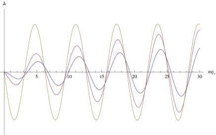
Figure 6: The function of $\Delta$ defined by Eq. (4.20) for $x_{0}=my_{0}=0.01,\;1.0,\;1000$, respectively. Note that the horizontal axis is $my_{c}$.

Table I shows the first three modes $m_{n}\;(n=1,2,3)$ for $x_{0}=0.01,\;1.0,\;1000$, from which we can see that to find $m_{n}$ it is sufficient to consider only the case where $x_{0}\gg 1$.

$x_{0}$	$m_{1}y_{c}$	$m_{2}y_{c}$	$m_{3}y_{c}$
0.01	3.55	6.72	9.87
1.0	3.25	6.41	9.56
1000	3.14	6.28	9.42

Table 1: The first three modes $m_{n}\;(n=1,2,3)$ for $x_{0}=0.01,\;1.0,\;1000$, respectively.

When $x_{0}\gg 1$ we find that $x_{c}=x_{0}+my_{c}\gg 1$, and that AS72

$$J_{\nu}(x) \simeq -Y_{\nu+1}(x)\simeq\sqrt{\frac{2}{\pi x}}\cos\left(x-\frac{7}{20}\pi\right),$$

$$Y_{\nu}(x) \simeq J_{\nu+1}(x)\simeq\sqrt{\frac{2}{\pi x}}\sin\left(x-\frac{7}{20}\pi\right).$$ (4.21)

Inserting the above expressions into Eqs. (IV.1.2) and (4.20), we obtain

$$\Delta = -\sqrt{\frac{4}{\pi^{2}x_{0}x_{c}}}\left\{10\left(x_{c}-x_{0}\right)\cos\left(x_{c}-x_{0}\right)\right.$$ (4.22)

$$\left.+\left(4+25x_{0}x_{c}\right)\sin\left(x_{c}-x_{0}\right)\right\},$$

whose roots are given by

$$\tan\left(x_{c}-x_{0}\right)=-\frac{10\left(x_{c}-x_{0}\right)}{4+25x_{0}x_{c}}.$$ (4.23)

From this equation, we can see that $m_{n}$ satisfies the bounds

$$\frac{n\pi}{y_{c}}<m_{n}<\frac{(n+1)\pi}{y_{c}},\;(n=1,2,3,...).$$ (4.24)

Combining the above expression with Table I, we find that $m_{n}$ is well approximated by

$$m_{n}\simeq n\pi\left(\frac{l_{pl}}{y_{c}}\right)M_{pl},$$ (4.25)

For $x_{0}\gg 1$. In particular, we have

$$m_{1} \simeq 3.14\times\left(\frac{10^{-19}\;{\mbox{m}}}{y_{c}}\right)\;{\mbox{TeV}}$$ (4.26)

$$\simeq \cases{1\;{\mbox{TeV}},&$y_{c}\simeq 10^{-19}\;{\mbox{m}}$,\cr 10^{-2}\;{\mbox{eV}},&$y_{c}\simeq 10^{-5}\;{\mbox{m}}$,\cr 10^{-4}\;{\mbox{eV}},&$y_{c}\simeq 10^{-3}\;{\mbox{m}}$.\cr}$$

It should be noted that the mass $m_{n}$ calculated above is measured by the observer with the metric $\eta_{\mu\nu}$. However, since the warped factor $e^{\sigma(y)}$ is not one at $y=y_{c}$, the physical mass on the visible brane should be given by RS1

$$m^{obs}_{n}=e^{-\sigma\left(y_{c}\right)}m_{n}=\left(\frac{y_{c}+y_{0}}{L}\right)^{1/5}m_{n}.$$ (4.27)

Without introducing any new hierarchy, we expect that $\left[({y_{c}+y_{0})}/{L}\right]^{1/5}\simeq{\cal{O}}(1)$. As a result, we have

$$m^{obs}_{n}=\left(\frac{y_{c}+y_{0}}{L}\right)^{1/5}m_{n}\simeq m_{n}.$$ (4.28)

For each $m_{n}$ that satisfies Eq. (4.20), the wavefunction $\psi_{n}(x)$ is given by

$$\psi_{n}(x) = N_{n}x^{1/2}\left\{\Delta_{12}\left(m_{n},y_{c}\right)J_{\nu}(x)\right.$$ (4.29)

$$\left.-\Delta_{11}\left(m_{n},y_{c}\right)Y_{\nu}(x)\right\},$$

where $N_{n}\equiv N_{n}\left(m_{n},y_{c}\right)$ is the normalization factor, so that

$$\int^{y_{c}}_{0}{\left|\psi_{n}(x)\right|^{2}dy}=1.$$ (4.30)

IV.2 4D Newtonian Potential and Yukawa Corrections

To calculate the four-dimensional effective Newtonian potential and its corrections, let us consider two point-like sources of masses $M_{1}$ and $M_{2}$, located on the brane at $y=y_{c}$. Then, the discrete eigenfunction $\psi_{n}(x)$ of mass $m_{n}$ has an Yukawa correction to the four-dimensional gravitational potential between the two particles BS99 ; Csaki00

$$U(r)=G_{4}\frac{M_{1}M_{2}}{r}+\frac{M_{1}M_{2}}{M_{5}^{3}r}\sum_{n=1}^{\infty}{e^{-m_{n}r}\left|\psi_{n}(x_{c})\right|^{2}},$$ (4.31)

where $\psi_{n}(x_{c})$ is given by Eq. (4.29). When $x_{0}=m_{n}y_{0}\gg 1$, from Eq. (IV.1.2) we find that

$$N_{n} \simeq \sqrt{\frac{\pi^{2}}{50x_{c}y_{c}}},$$

$$\psi_{n}(x_{c}) \simeq \sqrt{\frac{2}{y_{c}}}.$$ (4.32)

Then, it can be seen that all terms except for the first one in Eq. (4.31) are exponentially suppressed, and have negligible contributions to the 4D effective potential $U(r)$.

V Brane Cosmology

In this section, we shall apply the formulas developed in Section II to cosmology.

V.1 General Metric and Gauge Choices

The general metric for cosmology takes the form WS07 ; WCS08 ,

$$ds^{2}_{5}=g_{ab}dx^{a}dx^{b}=g_{MN}dx^{M}dx^{N}-e^{2\omega\left(x^{M}\right)}d\Sigma^{2}_{k},$$ (5.1)

where $M,\;N=0,1$, and

$$d\Sigma^{2}_{k}=\frac{dr^{2}}{1-kr^{2}}+r^{2}\left(d\theta^{2}+\sin^{2}\theta d\varphi^{2}\right),$$ (5.2)

where the constant $k$ represents the curvature of the 3-space, and can be positive, negative or zero. Without loss of generality, we shall choose coordinates such that $k=0,\pm 1$. The metric (5.1) is invariant under the coordinate transformations,

$${x^{\prime}}^{N}=f^{N}\left({x}^{M}\right).$$ (5.3)

Using these two degrees of freedom, one can choose different gauges.

V.1.1 The Canonical Gauge

In particular, in WCS08 the gauge was chosen such that

$$g_{01}=0,\;\;\;y_{I}=0,\;y_{c},$$ (5.4)

where $y_{I}$ denote the locations of the two orbifold branes, with $y_{c}$ being a constant. Then, the general metric can be cast in the form,

$$ds^{2}_{5}=N^{2}(t,|y|)dt^{2}-B^{2}(t,|y|)dy^{2}-B^{2}(t,|y|)d\Sigma^{2}_{k},$$ (5.5)

where $|y|$ is defined as that given in WCS08 [cf. Fig. 2]. By using distribution theory, the field equations on the two branes were obtained explicitly in terms of the discontinuities of the metric coefficients $A,\;B$ and $N$. For the details, we refer readers to WCS08 . The gauge Eq. (5.4) will be referred to as the canonical gauge.

V.1.2 The Conformal Gauge

One can also choose the gauge

$$g_{00}=g_{11},\;\;\;g_{01}=0,$$ (5.6)

so that the general five-dimensional metric takes the form,

$$ds^{2}_{5}=e^{2\sigma(t,y)}\left(dt^{2}-dy^{2}\right)-e^{2\omega(t,y)}d\Sigma^{2}_{k}.$$ (5.7)

But with this gauge, the hypersurfaces of the two branes are not fixed, and usually given by $y=y_{I}(t)$. We shall refer the gauge Eq. (5.6) to as the conformal gauge. It should be noted that in this conformal gauge, metric (5.7) still has the remaining gauge freedom,

$$t=f\left(\xi_{+}\right)+g\left(\xi_{-}\right),\;\;\;y=f\left(\xi_{+}\right)-g\left(\xi_{-}\right)$$ (5.8)

where $\xi_{\pm}\equiv t^{\prime}\pm y^{\prime}$, and $f\left(\xi_{+}\right)$ and $g\left(\xi_{-}\right)$ are arbitrary functions of their indicated arguments.

It should be noted that in Martin04 comoving branes were considered, and it was claimed that the gauge freedom of Eq. (5.8) can always bring the two branes at rest (comoving). However, from Eq. (A5) of Martin04 it can be seen that this is not true (at least) at the moment of the collision, $\tilde{y}_{2}(t)=0$, for which Eq. (A5) reduces to $f(t)=f(t)+2$, which is not satisfied for any finite function $f(t)$. In addition, using Eq. (5.8), one can always bring one brane at rest, as shown in Bowcock00 (See also Martin04 ). In this paper, we shall leave this possibility open, and choose to work with the conformal gauge, in which the branes are located on the surfaces $y=y_{I}(t)$.

V.2 Field Equations Outside the Two Branes

It can be shown that outside the two branes the field equations (II.2) for the metric (5.7) have four independent components, which can be cast in the form,

$$\omega_{,tt}+\omega_{,t}\left(\omega_{,t}-2\sigma_{,t}\right)+\omega_{,yy}+\omega_{,y}\left(\omega_{,y}-2\sigma_{,y}\right)$$ (5.11)

$$\;\;\;\;\;\;\;\;\;\;\;\;\;\;\;=-\frac{1}{6}\left({\phi_{,t}}^{2}+{\phi_{,y}}^{2}\right),$$

$$2\sigma_{,tt}+\omega_{,tt}-3{\omega_{,t}}^{2}-\left(2\sigma_{,yy}+\omega_{,yy}-3{\omega_{,y}}^{2}\right)$$

$$\;\;\;\;\;\;\;\;\;\;\;\;\;\;\;-4ke^{2(\sigma-\omega)}$$

$$\;\;\;\;\;\;\;\;\;\;\;\;\;\;\;=-\frac{1}{2}\left({\phi_{,t}}^{2}-{\phi_{,y}}^{2}\right),$$

$$\omega_{,ty}+\omega_{,t}\omega_{,y}-\left(\sigma_{,t}\omega_{,y}+\sigma_{,y}\omega_{,t}\right)$$

$$\;\;\;\;\;\;\;\;\;\;\;\;\;\;\;=-\frac{1}{6}\phi_{,t}\phi_{,y},$$

$$\omega_{,tt}+3{\omega_{,t}}^{2}-\left(\omega_{,yy}+3{\omega_{,y}}^{2}\right)+2ke^{2(\sigma-\omega)}$$ (5.12)

$$\;\;\;\;\;\;\;\;\;\;\;\;\;\;\;=2\alpha^{2}e^{2(\sigma-\phi)}.$$

On the other hand, the Klein-Gordon equation (2.20) takes the form,

$$\phi_{,tt}+3\phi_{,t}\omega_{,t}-\left(\phi_{,yy}+3\phi_{,y}\omega_{,y}\right)=12\alpha^{2}e^{2(\sigma-\phi)}.$$ (5.13)

V.3 Field Equations on the Two Branes

Eqs. (5.11) - (5.13) are the field equations that are valid in between the two orbifold branes,

$$y_{2}(t)<y<y_{1}(t).$$ (5.14)

The proper distance between the two branes is given by

$${\mathcal{D}}(t)=\int_{y_{2}}^{y_{1}}{e^{\sigma(t,y)}dy}.$$ (5.15)

On each of the two branes, the metric reduces to

$$\left.ds^{2}_{5}\right|_{M^{(I)}_{4}}=g^{(I)}_{\mu\nu}d\xi_{(I)}^{\mu}d\xi_{(I)}^{\nu}=d\tau_{I}^{2}-a^{2}\left(\tau_{I}\right)d\Sigma^{2}_{k},$$ (5.16)

where $\xi^{\mu}_{(I)}\equiv\left\{\tau_{I},r,\theta,\varphi\right\}$, and $\tau_{I}$ denotes the proper time of the I-th brane, defined by

$$d\tau_{I} = e^{\sigma\left[t_{I}(\tau_{I}),y_{I}(\tau_{I})\right]}\sqrt{1-\left(\frac{\dot{y}_{I}}{\dot{t}_{I}}\right)^{2}}\;dt_{I},$$

$$a\left(\tau_{I}\right) \equiv e^{\omega\left[t_{I}(\tau_{I}),y_{I}(\tau_{I})\right]},$$ (5.17)

with $\dot{y}_{I}\equiv d{y}_{I}/d\tau_{I}$, etc. For the sake of simplicity and without of causing any confusion, from now on we shall drop all the indices “I”, unless some specific attention is needed. Then, the normal vector $n_{a}$ and the tangential vectors $e^{a}_{(\mu)}$ are given, respectively, by

$$n_{a} = e^{2\sigma}\left(-\dot{y}\delta^{t}_{a}+\dot{t}\delta^{y}_{a}\right),$$

$$n^{a} = -\left(\dot{y}\delta^{a}_{t}+\dot{t}\delta^{a}_{y}\right),$$

$$e^{a}_{(\tau)} = \dot{t}\delta^{a}_{t}+\dot{y}\delta^{a}_{y},\;\;\;e^{a}_{(r)}=\delta^{a}_{r},$$

$$e^{a}_{(\theta)} = \delta^{a}_{\theta},\;\;\;e^{a}_{(\varphi)}=\delta^{a}_{\varphi}.$$ (5.18)

Thus, we find that

$${\mathcal{G}}^{(5)}_{\mu\nu} = {\mathcal{G}}^{(5)}_{\tau}\delta^{\tau}_{\mu}\delta^{\tau}_{\nu}-{\mathcal{G}}^{(5)}_{\theta}\delta^{m}_{\mu}\delta^{n}_{\nu}g_{mn},$$

$$E^{(5)}_{\mu\nu} = E^{(5)}\left(3\delta^{\tau}_{\mu}\delta^{\tau}_{\nu}-\delta^{m}_{\mu}\delta^{n}_{\nu}g_{mn}\right),$$ (5.19)

where $m,\;n=r,\;\theta,\;\varphi$, and

$${\mathcal{G}}^{(5)}_{\tau} \equiv \frac{1}{3}e^{-2\sigma}\left({\phi_{,t}}^{2}-{\phi_{,y}}^{2}\right)-\frac{1}{24}\left(5\left(\nabla\phi\right)^{2}-6V_{5}\right),$$

$${\mathcal{G}}^{(5)}_{\theta} \equiv \frac{1}{24}\left(8{\phi_{,n}}^{2}+5\left(\nabla\phi\right)^{2}-6V_{5}\right),$$

$$E^{(5)} \equiv \frac{1}{6}e^{-2\sigma}\left(\left(\sigma_{,tt}-\omega_{,tt}\right)-\left(\sigma_{,yy}-\omega_{,yy}\right)\right.$$ (5.20)

$$\left.+ke^{2(\sigma-\omega)}\right),$$

with

$$V_{5}\equiv 6\alpha^{2}e^{-2\phi}.$$ (5.21)

Then, it can be shown that the four-dimensional field equations on each of the two branes take the form,

$$H^{2} + \frac{k}{a^{2}}=\frac{8\pi G}{3}\left(\rho+\tau_{\phi}\right)+\frac{1}{3}\Lambda+\frac{1}{3}{\mathcal{G}}^{(5)}_{\tau}+E^{(5)}$$ (5.22)

$$+\frac{2\pi G}{3\rho_{\Lambda}}\left(\rho+\tau_{\phi}\right)^{2},$$

$$\frac{\ddot{a}}{a} = -\frac{4\pi G}{3}\left(\rho+3p-2\tau_{\phi}\right)+\frac{1}{3}\Lambda$$ (5.23)

$$-E^{(5)}-\frac{1}{6}\left({\mathcal{G}}^{(5)}_{\tau}+3{\mathcal{G}}^{(5)}_{\theta}\right)-\frac{2\pi G}{3\rho_{\Lambda}}\left[\rho\left(2\rho+3p\right)\right.$$

$$\left.+\left(\rho+3p-\tau_{\phi}\right)\tau_{\phi}\right],$$

where $H\equiv\dot{a}/{a},,\;\Lambda\equiv\Lambda_{4},\;G\equiv G_{4}$ and $\rho_{\Lambda}=\Lambda/(8\pi G)$.

On the other hand, from Eqs. (2.45) and (2.46) we find that

$$\phi_{,n}^{(I)}=\epsilon_{I}\left(\kappa^{2}_{5}\frac{\partial V^{(I)}_{4}}{\partial\phi}-6\alpha\epsilon_{I}e^{-\phi}+\frac{1}{2}\sigma^{(I)}_{\phi}\right),\;\;$$ (5.24)

$$\left(\dot{\rho}^{(I)}+\dot{\tau}^{(I)}_{\phi}\right)+3H^{(I)}\left(\rho^{(I)}+p^{(I)}\right)=\Pi^{(I)},\;\;\;\;$$ (5.25)

where $H^{(I)}\equiv\left[da\left(\tau_{I}\right)/d\tau_{I}\right]/a\left(\tau_{I}\right)$, and

$$\Pi^{(I)}\equiv\frac{\epsilon_{I}}{\kappa^{2}_{5}}\phi^{(I)}_{,\tau}\phi^{(I)}_{,n}.$$ (5.26)

From Eqs. (2.11) and (V.3), we also find that

$$\dot{\tau}^{(I)}_{\phi}=\frac{\phi^{(I)}_{,\tau}}{\kappa^{2}_{5}}\left\{\kappa^{2}_{5}\frac{\partial V^{(I)}_{4}}{\partial\phi}-6\alpha\epsilon_{I}e^{-\phi}\right\}.$$ (5.27)

Then, Eqs. (5.24) and (5.25) can be written as

$$\dot{\tau}^{(I)}_{\phi}=\Pi^{(I)}-Q^{(I)},$$ (5.28)

$$\dot{\rho}^{(I)}+3H^{(I)}\left(\rho^{(I)}+p^{(I)}\right)=Q^{(I)},$$ (5.29)

where

$$Q^{(I)}\equiv\frac{1}{2\kappa^{2}_{5}}\phi^{(I)}_{,\tau}\sigma^{(I)}_{\phi}.$$ (5.30)

When there is only gravitational interaction between the scalar field and the perfect fluid, we have $\sigma_{\phi}^{(I)}=0$ [cf. Es.(2.18)], and then the above equations reduce to

$$\dot{\tau}^{(I)}_{\phi}=\Pi^{(I)},\;\left(Q^{(I)}=0\right),$$ (5.31)

$$\dot{\rho}^{(I)}+3H^{(I)}\left(\rho^{(I)}+p^{(I)}\right)=0,\;\left(Q^{(I)}=0\right).\;\;\;\;\;$$ (5.32)

Eqs.(4.14a)-(4.14d) form the complete set of the field equations on the branes. However, in order to solve them, additional information from bulk is needed. In particular, the $E^{(5)}$ term represents the projection of the five-dimensional Weyl tensor on the branes, while the ${\cal{G}}^{(5)}_{\tau}$ and ${\cal{G}}^{(5)}_{\theta}$ terms represent the contribution of the bulk scalar field. When the bulk is conformally flat, $E^{(5)}$ vanishes. The bulk scalar contributions are in general always present, although in some particular cases, such contributions might be negligible. Then, from Eqs.(4.14a) and (4.14b) we can see that the universe will be asymptotically approaching to the $\Lambda$CDM model for $\rho,\;\tau_{\phi}\ll 1$ at later time $a\gg 1$. It should be noted that in GWW07 , using the large extra dimensions, we showed that the effective cosmological constant $\Lambda$ can be lowered to its observational value. In the early universe, the quadratic terms of $\rho$ will dominate, and $H\propto\rho$, a feature that is commonly shared by brane-world models branes .

VI Conclusions and discussions

In this paper, we have systematically studied the brane world in the in the framework of the Horava-Witten heterotic M-Theory on $S^{1}/Z_{2}$ along the line set up by Lukas et al HW96 ; LOSW99 . In particular, after reviewing the model in Sec. II, and writing separately down the general gravitational and matter field equations both in the bulk and on the branes, In Sec. III, we have shown explicitly that the radion is stable, by using the Goldberger-Wise mechanism GW99 . After working out the specific relation between the distance, $Y_{c}$, of the two branes and the radion $\varphi$, we have obtained an explicit form of the radion mass $m_{\varphi}$ in terms of the relevant parameters of the model [cf. Eq.(3.37)]. By properly choosing these parameters, it can be seen that the radion mass can be of the order of GeV.

We have also shown that the gravity is localized on the visible (TeV) brane [cf. Sec. IV], in contrast to the RS1 model in which the gravity is localized on the Planck (hidden) brane RS1 . In addition, the spectrum of the gravitational KK modes is discrete, and given explicitly by Eq.(4.25), which can be in the order of TeV. The corrections to the 4D Newtonian potential from the higher order gravitational KK modes are exponentially suppressed and can be safely neglected [cf. Eq.(4.31)].

To apply such a setup to cosmology, we have first found the general form of metric, by embedding a constant curvature 3-space into a five-dimensional bulk, and discussed the gauge conditions in details. Working with the conformal gauge, we have written down the general gravitational and matter field equations in the bulk, given by Eqs.(5.11)-(5.13), and the generalized Friedmann-like equations on each of the two orbifold branes, given by Eqs.(5.22) and (5.23). The conservation laws for the scalar and matter fields are given, respectively, by Eqs.(5.24) and (5.25). These consist of the complete set of field equations of the brane cosmology in the framework of the Horava-Witten heterotic M-Theory on $S^{1}/Z_{2}$ along the line set up by Lukas et al HW96 ; LOSW99 .

In the study of brane worlds, one of the most attractive features is that it may resolve the long standing hierarchy problem, namely the large difference in magnitudes between the Planck and electroweak scales, ${M_{pl}}/{M_{EW}}\simeq 10^{16}$, where $M_{EW}$ denotes the electroweak scale with $M_{EW}\sim TeV$. In particular, using the large extra dimensions, ADD found that in a D-dimensional bulk with the Planck scale $M_{D}$, the deduced 4-dimensional Planck mass $M_{pl}$ ADD98 is given by $M_{pl}^{2}=V_{D-4}M_{D}^{D-2}$, where $V_{D-4}$ denotes the volume of the extra (D-4)-dimensional space. Clearly, if the extra dimensions are large enough, even $M_{D}$ is in the order of electroweak scale $M_{D}\simeq M_{EW}\simeq TeV$, one can get the correct order of $M_{pl}\simeq 10^{16}\;TeV$, whereby the hierarchy problem is resolved. In the RS1 model, the mechanism is completely different RS1 . Instead of using large dimensions, RS used the warped factor $\sigma(y)=k|y|$, for which the mass $m_{0}$ measured on the invisible (Planck) brane is related to the mass $m$ measured on the visible (TeV) brane by $m=e^{-ky_{c}}m_{0}$. Clearly, by properly choosing the distance $y_{c}$ between the two branes, one can lower $m$ to the order of $TeV$, even $m_{0}$ is still in the roder of $M_{pl}$. It should be noted that the five-dimensional Planck mass $M_{5}$ in the RS1 sceanrio is still of the order of $M_{pl}$ and the two are related by $M^{2}_{pl}={M^{3}}{k^{-1}}\left(1-e^{-2ky_{c}}\right)\simeq M^{2}_{5}$ for $k\simeq M_{5}$.

It is important to note that, when deriving the relation between $M_{D}$ and $M_{pl}$, in both scenarios it was implicitly assumed that the 4-dimensional effective Einstein-Hilbert action $S_{g}^{eff.}$ couples with matter directly as

$$S_{g}^{eff.}+S_{m}=\int{\sqrt{-g}d^{4}\left(-\frac{1}{2\kappa^{2}_{4}}R+{\cal{L}}_{m}\right)},$$ (6.1)

from which one obtains the Einstein field equations, $G_{\mu\nu}=\kappa^{2}_{4}\tau_{\mu\nu}$. In the weak field limit, one arrives at $\kappa^{2}_{4}=8\pi G/c^{4}$ Inverno . However, in the brane-world scenarios, the coupling between the curvature and matter is much more complicated than that given by the above equation. In particular, the gravitational field equations on the branes are given by Eq.(2.30), which is a second-order polynomial in terms of the energy-momentum tensor $\tau_{\mu\nu}$ of the brane. In the weak-field regime, the quadratic terms are negligible, and the term linear to $\tau_{\mu\nu}$ dominates. Then, under the weak-field limit, one can show that $\kappa^{2}_{4}$ defined by Eq.(2.32) is related to the Newtonian constant exactly by $\kappa^{2}_{4}=8\pi G/c^{4}$, from which we find that

$$g_{k}=\frac{6\kappa^{2}_{4}}{\kappa^{4}_{5}}.$$ (6.2)

Note that this result is quite general, and applicable to a large class of brane-world scenarios branes . In the present case, we have $\kappa^{2}_{5}=M^{-3}_{5}=1/(M^{9}_{11}R^{6})$, where $R$ is the typical size of the extra dimensions GWW07 . Then, one find that $g_{k}\simeq 10^{-47}\;GeV^{4}$, that is, to solve the hierarchy problem in the framework of the HW heterotic M Theory on $S^{1}/Z_{2}$, the tension of the brane has to be in the same order of the current matter $\rho_{m}$, as well as of the observational cosmological constant $\rho_{\Lambda}^{obs}$, of course.

Finally, we would like to note that, when we considered the radion stability, the backreaction of the Goldberger-Wise field $\Phi$ was not taken into account. In the Randall-Sandrum model RS1 , it was shown that such effects do not change the main conclusions of the stability of radion DeWolfe . It would be very interesting to show that it is also the case here. It is also very important to study constraints from other physical considerations, such as the solar system tests, the formation of large-scale structure, and the early universe.

- (1) A.G. Riess et al., Astron. J. 116, 1009 (1998); S. Perlmutter et al., Astrophys. J. 517, 565 (1999).
- (2) A.G. Riess et al., Astrophys. J. 607, 665 (2004); P. Astier et al., Astron. and Astrophys. 447, 31 (2006); D.N. Spergel et al., astro-ph/0603449; W.M. Wood-Vasey et al., astro-ph/0701041; T.M. Davis et al., astro-ph/0701510; E. Komatsu, et al, Astrophys. J. Suppl. 180, 330 (2009) [arXiv:0803.0547].
- (3) S. Sullivan, A. Cooray, and D.E. Holz, arXiv:0706.3730; A. Mantz, et al., arXiv:0709.4294; J. Dunkley, et al., arXiv:0803.0586; and E. Komatsu, et al., arXiv:0803.0547.
- (4) S. Weinberg, Rev. Mod. Phys. 61, 1 (1989); S.M. Carroll, arXiv:astro-ph/0004075; T. Padmanabhan, Phys. Rept. 380, 235 (2003); S. Nobbenhuis, arXiv:gr-qc/0411093; J. Polchinski, arXiv:hep-th/0603249; and J.M. Cline, arXiv:hep-th/0612129.
- (5) W. Fischler, et al., JHEP, 07, 003 (2001); J.M. Cline, ibid., 08, 035 (2001); E. Halyo, ibid., 10, 025 (2001); and S. Hellerman, ibid., 06, 003 (2003).
- (6) L.M. Krauss and R.J. Scherrer, Gen. Relativ. Grav. 39, 1545 (2007); and references therein.
- (7) R. R. Caldwell, R. Dave and P. J. Steinhardt, Phys. Rev. Lett. 80, 1582 (1998); A. R. Liddle and R. J. Scherrer, Phys. Rev. D59, 023509 (1999); and P. J. Steinhardt, L. M. Wang and I. Zlatev, ibid., 59, 123504 (1999).
- (8) G. R. Dvali, G. Gabadadze and M. Porrati, Phys. Lett. B484, 112 (2000); C. Deffayet, ibid., 502, 199 (2001); and V. Sahni and Y. Shtanov, JCAP, 0311, 014 (2003).
- (9) S. Capozziello, S. Carloni, and A. Troisi, arXiv:astro-ph/0303041; S.M. Carroll, et al, Phys. Rev. D70, 043528 (2003); and S. Nojiri and S.D. Odintsov, ibid., 68, 123512 (2003).
- (10) E.J. Copeland, M. Sami and S. Tsujikawa, Int. J. Mod. Phys. D15, 1753 (2006); J. Frieman, M. Turner, and D. Huterer, arXiv:0803.0982; R. Durrer and R. Maartens, arXiv:0811.4132; and references therein.
- (11) L. Susskind, arXiv:hep-th/0302219.
- (12) R. Bousso and J. Polchinski, JHEP, 006, 006 (2000).
- (13) P.K. Townsend and N.R. Wohlfarth, Phys. Rev. Lett. 91, 061302 (2003).
- (14) G. W.Gibbons in Supersymmetry, Supergravity and Related Topics, edited by F. de Aguila, et al (Sigapore, World Scientific, 1985), p.124; and J.M. Maldacena and C. Nuñez, Int. J. Mod. Phys. A16, 822 (2001).
- (15) N. Ohta, Phys. Rev. Lett. 91, 061303 (2003).
- (16) N.R. Wohlfarth, Phys. Lett. B563, 1 (2003); and S. Roy ibid., 567, 322 (2003).
- (17) J.K. Webb, et al, Phys. Rev. Lett. 87, 091301 (2001); J.M. Cline and J. Vinet, Phys. Rev. D68, 025015 (2003); N. Ohta, Prog. Theor. Phys. 110, 269 (2003); Int. J. Mod. Phys. A20, 1 (2005); C.M. Chen, et al, JHEP, 10, 058 (2003); E. Bergshoeff, Class. Quantum Grav. 21, 1947 (2004); J.-L. Lehners, P. Smyth, K.S. Stelle, ibid., 22, 2589 (2005); Y. Gong and A. Wang, ibid., 23, 3419 (2006); I.P. Neupane and D.L. Wiltshire, Phys. Rev. D72, 083509 (2005); Phys. Lett. B619, 201 (2005); K. Maeda and N. Ohta, ibid., B597, 400 (2004); Phys. Rev. D71, 063520 (2005); K. Akune, K. Maeda and N. Ohta, ibid., 103506 (2006); V. Baukh and A. Zhuk, ibid., 73, 104016 (2006); A. Krause, Phys. Rev. Lett. 98, 241601 (2007); I.P. Neupane, ibid., 98, 061301 (2007); J.-L. Lehners, P. Smyth, K.S. Stelle, Nucl. Phys. B790, 89 (2008); and references therein.
- (18) Y.-G. Gong, A. Wang, and Q. Wu, Phys. Lett. B663, 147 (2008) [arXiv:0711.1597].
- (19) H. Horava and E. Witten, Nucl. Phys. B460, 506 (1996); 475, 94 (1996).
- (20) N. Arkani-Hamed, S. Dimopoulos and G. Dvali, Phys. Lett. B429, 263 (1998); Phys. Rev. D59, 086004 (1999); and I. Antoniadis, et al., Phys. Lett., B436, 257 (1998).
- (21) A. Wang and N.O. Santos, Phys. Lett. B669, 127 (2008) [arXiv:0712.3938]; and arXiv:0808.2055.
- (22) Q. Wu, N.O. Santos, P. Vo, and A. Wang, JCAP 09, 004 (2008) [arXiv:0804.0620].
- (23) A. Wang and N.O. Santos, in preparation.
- (24) W.D. Goldberger and M.B. Wise, Phys. Rev. Lett. 83, 4922 (1999).
- (25) A. Lukas, et al., Phys. Rev. D59, 086001 (1999); Nucl. Phys. B552, 246 (1999).
- (26) V.A. Rubakov, Phys. Usp. 44, 871 (2001); S. Förste, Fortsch. Phys. 50, 221 (2002); C.P. Burgess, et al, JHEP, 0201, 014 (2002); E. Papantonopoulos, Lect. Notes Phys. 592, 458 (2002); R. Maartens, Living Reviews of Relativity 7 (2004); P. Brax, C. van de Bruck and A. C. Davis, Rept. Prog. Phys. 67, 2183 (2004) [arXiv:hep-th/0404011]; U. Günther and A. Zhuk, “Phenomenology of Brane-World Cosmological Models,” arXiv:gr-qc/0410130 (2004); P. Brax, C. van de Bruck, and A.C. Davis, “Brane World Cosmology,” Rept. Prog. Phys. 67, 2183 (2004) [arXiv:hep-th/0404011]; V. Sahni, “Cosmological Surprises from Braneworld models of Dark Energy,” arXiv:astro-ph/0502032 (2005); R. Durrer, “Braneworlds,” arXiv:hep-th/0507006 (2005); D. Langlois, “Is our Universe Brane,” arXiv:hep-th/0509231 (2005); A. Lue, “Phenomenology of Dvali-Gabadadze-Porrati Cosmologies,” Phys. Rept. 423, 1 (2006) [arXiv:astro-ph/0510068]; D. Wands, “Brane-world cosmology,” arXiv:gr-qc/0601078 (2006); and R. Maartens, “Dark Energy from Brane-world Gravity,” arXiv:astro-ph/0602415 (2006).
- (27) W. Chen, et al, Nucl. Phys. B732, 118 (2006); and J.-L. Lehners, P. McFadden, and N. Turok, Phys. Rev. D75, 103510 (2007).
- (28) C. Csaki, J. Erlich, and C. Grojean, Gen. Relativ. Grav. 33, 1921 (2001).
- (29) N. Arkani-Hamed, et al, Phys. Lett. B480, 193 (2000); and S. Kachru, M.B. Schulz, and E. Silverstein, Phys. Rev. D62, 045021 (2000).
- (30) Y. Aghababaie, et al, Nucl. Phys. B680, 389 (2004); JHEP, 0309, 037 (2003); C.P. Burgess, Ann. Phys. 313, 283 (2004); AIP Conf. Proc. 743, 417 (2005); and C.P. Burgess , J. Matias, and F. Quevedo, Nucl.Phys. B706, 71 (2005).
- (31) S. Forste, et al, Phys. Lett. B481, 360 (2000); JHEP, 0009, 034 (2000); C. Csaki, et al, Nucl. Phys. B604, 312 (2001); and J.M. Cline and H. Firouzjahi, Phys. Rev. D65, 043501 (2002).
- (32) K. Koyama, arXiv:0706.1557.
- (33) C.P. Burgess, arXiv:0708.0911.
- (34) K. Benakli, Int. J. Mod. Phys. D8, 153 (1999); H.S. Reall, Phys. Rev. D59, 103506 (1999); and A. Lukas, B.A. Ovrut, and D. Waldram, ibid., 60, 086001 (1999).
- (35) J. Cline, C. Grojean, and G. Servant, Phys. Rev. Lett. 83, 4245 (1999); C. Csaki et al, Phys. Lett. B462, 34 (1999).
- (36) G.W. Gibbons and S.W. Hawking, Phys. Rev. D12, 2752 (1977).
- (37) S.C. Davis, Phys. Rev. D67, 024030 (2003).
- (38) D. Konikowska, M. Olechowski, and M.G. Schmidt, Phys. Rev. D73, 105018 (2006).
- (39) C. Lanczos, Phys. Z. 23, 539 (1922); Ann. Phys. (Germany), 74, 518 (1924).
- (40) W. Israel, Nuovo Cim. 44B, 1 (1966); ibid., 48B, 463 (1967).
- (41) F. Leblond, R.C. Myers, and D.J. Winters, JHEP, 07, 031 (2001).
- (42) A. Wang, R.-G. Cai, and N.O. Santos, Nucl. Phys. B797, 395 (2008) [arXiv:astro-ph/0607371].
- (43) T. Shiromizu, K.-I. Maeda, and M. Sasaki, Phys. Rev. D62, 024012 (2000); and R.-G. Cai and L.-M. Cao, Nucl. Phys. B785, 135 (2007).
- (44) A.N. Aliev and A.E. Gumrukcuoglu, Class. Quantum Grav. 21, 5081 (2004).
- (45) L. Randall and R. Sundrum, Phys. Rev. Lett. 83, 3370 (1999).
- (46) M. Abramowitz and I.A. Stegun, Handbook of Mathematical Functions (Dover Publications, INC., New York, 1972), pp.374-8.
- (47) W.D. Goldberger and M.B. Wise, Phys. Lett. B475, 275 (2000).
- (48) C. Charmousis, R. Gregory, and V. A. Rubakov, Phys.Rev. D62, 067505 (2000) [arXiv:hep-th/9912160].
- (49) J. Garriga and T. Tanaka, Phys. Rev. Lett. 84, 2778 (2000); T. Tanaka and X. Montes, Nucl. Phys. B582, 259 (2000).
- (50) L. Randall and R. Sundrum, Phys. Rev. Lett. 83, 4690 (1999).
- (51) C. Csaki, J. Erlich, T. J. Hollowwood, and Y. Shirman, Nucl. Phys. B581, 309 (2000).
- (52) C. Csaki, M.L. Graesser, and G.D. Kribs, Phys. Rev. D63, 065002 (2001).
- (53) A. Brandhuber and K. Sfetsos, JHEP, 10, 013 (1999).
- (54) J. Martin, G.N. Felder, A.V. Frolov, M. Peloso, and L.A. Kofman, Phys. Rev. D69, 084017 (2004).
- (55) P. Bowcock, C. Charmousis, and R. Gregory, Class. Quantum Grav. 17, 4745 (2000).
- (56) R. d’Inverno, Introducing Einstein’s Relativity (Clarendon Press, Oxford, 2003), pp.167-168.
- (57) O. DeWolfe et al, Phys. Rev. D62, 046008 (2000); and L. Kofman, J. marin, and M. Peloso, ibid., 70, 085015 (2004).