Admittance and noise in an electrically driven nano-structure: Interplay between quantum coherence and statistics

Abstract

We investigate the interplay between the quantum coherence and statistics in electrically driven nano-structures. We obtain expression for the admittance and the current noise for a driven nano-capacitor in terms of the Floquet scattering matrix and derive a non-equilibrium fluctuation-dissipation relation. As an interplay between the quantum phase coherence and the many-body correlation, the admittance has peak values whenever the noise power shows a step as a function of near-by gate voltage. Our theory is demonstrated by calculating the admittance and noise of driven double quantum dots.

Quantum dynamics in time-dependent potential is an important topic because of its unrevealed non-equilibrium phenomena as well as the increasing demand of manipulating coherent electronic states in quantum information sciencefeve ; gabelli . While the time-dependent potentials in diffusive conductors are known to have destructive role on the quantum coherence of electrons, it is not always obvious which role is played on the quantum coherence by the time-periodic potential in ballistic nano-structures. Quantum coherence and quantum many-particle statistics of relevant particles are key concepts to understand the electron transport properties. For instance, the current noise, which is basically two-particle property, contains the information on the quantum many-particle statisticsblanter . Furthermore, the noise of a coherent conductor in the presence of time-periodic external field is known to be sensitive to the phase of transmission amplitudesLevitov ; Lamacraft ; camalet .

In this work, we study how the interplay between the quantum coherence and the statistics affects on the transport properties in the presence of time-periodic external potential. We particularly concentrate on the noise of quantum displacement current through the driven capacitor, because in usual conductors, Shot noise (in classical granular nature of electrons) dominates other types of noises. By this means, we derive the analytic expression for the admittance and noise formula in terms of the Floquet scattering matrix for the driven nano-capacitor.

The linear response of the capacitor is described by the admittance $g(\omega)=I(\omega)/V(\omega)$ which relates the displacement current $I(\omega)$ to the applied voltage between capacitor $V(\omega)$. The expression which relates equilibrium admittance and the noise power $S(\omega)$ to the scattering matrix has been obtained by Büttiker and his coworkers buttiker ; nigg . Here we generalize the expression to the case of the non-equilibrium states generated by time-periodic potential of frequency $\Omega\gg\omega$. It will be shown here that, as in the case of equilibrium capacitors, the admittance of the driven capacitor can be also understood in terms of the time delay of electrons near Fermi level. Meanwhile, the non-equilibrium current noise power can not be understood within single-particle picture. The noise power shows step structure as a function of the nearby gate voltage, which is associated with the opening of temporal channels in the lead.

Let us begin by introducing a model for the system of a biased dynamic capacitor.(See Fig. 1.) A time-dependent potential with frequency $\Omega$ is applied in a nano-structure (box of dotted line) which is connected to a mesoscopic conductor. The chemical potential of the mesoscopic conductor is controlled by a nearby gate voltage $V_{g}$. The oscillating nano-structure and the mesoscopic conductor are in a loop enclosing a time-periodic magnetic flux $\Phi(t)$. The bias voltage $V(t)$ between nano-structure and external lead is induced as an electromotive force along the loop, $V(t)=d\Phi/dt=V(\omega)e^{i\omega t}$+c.c.

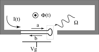
Figure 1: A time-periodic driven nanostructure (dotted box) is connected to a mesoscopic conductor. For bias voltage, an external loop driven by slow-varying flux $\Phi(t)=\Phi_{\omega}\cos\omega t$ is connected.

We assume the mesoscopic conductor is spatially one-dimensional and the electrons are non-interacting spin-polarized gas for simple presentation. Generalization of our results to the case of multi-channel conductors with spin is straightforward. The Hamiltonian for the conductor reads

$$H_{0}=\int d\epsilon~{}~{}\epsilon~{}~{}(a^{\dagger}(\epsilon)a(\epsilon)+b^{\dagger}(\epsilon)b(\epsilon)),$$ (1)

where $a(\epsilon)(b(\epsilon))$ is the annihilation operator for the incoming (outgoing) electron to the driven nano-structure; $\{a^{\dagger}(\epsilon),a(\epsilon^{\prime})\}=\{b^{\dagger}(\epsilon),b(\epsilon^{\prime})\}=\delta(\epsilon-\epsilon^{\prime})$, $\{a(\epsilon),a(\epsilon^{\prime})\}=\{b(\epsilon),b(\epsilon^{\prime})\}=\{a(\epsilon),b^{(\dagger)}(\epsilon^{\prime})\}=0$.

A time-periodic steady states are formed in the conductor and the driven nano-structure

$$i\hbar\frac{\partial}{\partial t}|\psi_{\epsilon}(t)\rangle=(H_{0}+H_{\Omega}(t)+H_{c})|\psi_{\epsilon}(t)\rangle,$$ (2)

where $H_{\Omega}$ is the time-periodic Hamiltonian for the electron in the driven nano-structure and $H_{c}$ denotes the coupling between the lead and the nano-structure. $|\psi_{\epsilon}(t)\rangle$ is formed by incoming electron state of energy $\epsilon$ and the linear combinations of its scattered states with energy $\epsilon+n\hbar\Omega$. We assume the external metallic lead is big enough so that it can be considered as a reservoir in thermal equilibrium. The occupation number for the incoming electron state of energy $\epsilon$ is given by Fermi-Dirac distribution function $f(\epsilon)$.

Let us consider the linear response of the electric current to the time-dependent magnetic flux. The perturbing time-dependent Hamiltonian is $H_{\omega}(t)=\Phi(t)\hat{I}$ where $\hat{I}$ is the current operator

$$\hat{I}=\frac{e}{h}\int d\epsilon d\epsilon^{\prime}~{}(a^{\dagger}(\epsilon)a(\epsilon^{\prime})-b^{\dagger}(\epsilon)b(\epsilon^{\prime})).~{}$$ (3)

In fact, the above current formula is an approximation where the current value is taken as the spatial average value over the length of the conductor $L$. This approximation holds when the relevant frequency scale is much smaller than the Fermi velocity divided by the length of the conductor $L$, i.e. $\omega,\Omega\ll v_{F}/L$, so that the relevant wavenumber $k$ satisfies $|k-k_{F}|L\ll 1$, and $k_{F}L\gg 1$ where the rapidly oscillating phase terms are washed out.

The adiabatic turning on of $\Phi(t)=\Phi_{\omega}\cos\omega te^{0^{+}t}$ gradually deforms $|\psi_{\epsilon}(t)\rangle$ to $|\Psi_{\epsilon}(t)\rangle=\int d\epsilon^{\prime}C_{\epsilon\epsilon^{\prime}}(t)|\psi_{\epsilon^{\prime}}(t)\rangle.$ The coefficients $C_{\epsilon\epsilon^{\prime}}(t)$ are determined by solving the Schrödinger equation for the time-dependent Hamiltonian $H(t)=H_{0}+H_{\Omega}(t)+H_{c}+H_{\omega}(t)$. By employing a perturbation expansion of $C_{\epsilon\epsilon^{\prime}}$ in terms of $\Phi_{\omega}$, we get the first order term $C^{(1)}_{\epsilon\epsilon^{\prime}}=\frac{\Phi_{\omega}}{i\hbar}\int^{t}_{-\infty}dt^{\prime}\cos\omega t^{\prime}\langle\psi_{\epsilon^{\prime}}(t^{\prime})|\hat{I}|\psi_{\epsilon}(t^{\prime})\rangle$.

Up to first order of $\Phi_{\omega}$, the $\omega$ component of the displacement current, $I^{(1)}_{\epsilon,\omega}$, is obtained through

$$\langle\Psi_{\epsilon}(t)|\hat{I}|\Psi_{\epsilon}(t)\rangle = \int d\epsilon^{\prime}\langle\psi_{\epsilon}(t)|\hat{I}|\psi_{\epsilon^{\prime}}(t)\rangle C^{(1)}_{\epsilon\epsilon^{\prime}}(t)+{\rm c.c.}$$ (4)

$$\approx I^{(1)}_{\epsilon,\omega}e^{i\omega t}+I^{(1)}_{\epsilon,-\omega}e^{-i\omega t}.$$

Floquet theorem says, the eigenstates $|\psi_{\epsilon}(t)\rangle$ of time-periodic Hamiltonian can be written in terms of time-independent basis $|\phi^{(l)}_{\epsilon}\rangle$ as $|\psi_{\epsilon}(t)\rangle=\exp(-i\frac{\epsilon}{\hbar}t)\sum_{l=-\infty}^{\infty}e^{-il\Omega t}|\phi^{(l)}_{\epsilon}\rangle$. Using Eqs.(3,4), one can relate $I^{(1)}_{\epsilon,\omega}$ to the Floquet eigenstates $|\phi^{(l)}_{\epsilon}\rangle$, which is useful for further calculations. The thermal-averaged displacement current is given by $I(\omega)=\int d\epsilon~{}f(\epsilon)~{}I^{(1)}_{\epsilon,\omega}$ because the incoming electrons are from the reservoir in equilibrium.

The admittance is given by the induced displacement current $I(\omega)$ divided by the applied voltage $V(\omega)=i\omega\Phi_{\omega}/2$. After some algebra we find;

$$g(\omega) = \frac{1}{i\omega}\sum_{m}\int d\epsilon d\epsilon^{\prime}|\sum_{l}\langle\phi^{(l)}_{\epsilon}|\hat{I}|\phi^{(l+m)}_{\epsilon^{\prime}}\rangle|^{2}$$

$$\times \frac{f(\epsilon)-f(\epsilon^{\prime})}{\epsilon-\epsilon^{\prime}-\hbar\omega-m\hbar\Omega+i0^{+}}.$$

Here, $|\omega|<|\Omega|$ is assumed.

In a quantum conductor with a time-periodic scatterer, the scattering relation between the incoming electron of energy $\epsilon$ and the out-going electron of energy $\epsilon^{\prime}$ is given by Floquet scattering matrixmoskalets , $S_{F}(\epsilon^{\prime},\epsilon)$. The Floquet state in the quantum conductor can be written

$$|\phi_{\epsilon}^{(l)}\rangle=(a^{\dagger}(\epsilon)\delta_{l0}+s_{l}(\epsilon)b^{\dagger}(\epsilon+l\hbar\Omega))|0\rangle,$$ (5)

where $s_{l}(\epsilon)=S_{F}(\epsilon+l\hbar\Omega,\epsilon)$. The unitarity of the scattering matrix gives $\sum_{l}|s_{l}(\epsilon)|^{2}=1$ and its time-reversal symmetry gives $s_{-l}(\epsilon+l\hbar\Omega)=s_{l}(\epsilon)$. The current matrix element in the Floquet basis simply reads

$$\langle\phi^{(l)}_{\epsilon}|\hat{I}|\phi^{(l+m)}_{\epsilon^{\prime}}\rangle=\frac{e}{h}\Big{(}\delta_{l,0}\delta_{m,0}-s^{*}_{l}(\epsilon)s_{l+m}(\epsilon^{\prime})\Big{)}$$ (6)

The real part of the admittance $g^{\prime}(\omega)$ is now written using $\frac{1}{x+i0^{+}}=P\frac{1}{x}-i\pi\delta(x)$;

$$g^{\prime}(\omega) = \frac{e^{2}}{2h}\sum_{m}\int d\epsilon\Big{|}\delta_{m0}-\sum_{l}s_{l+m}(\epsilon)s_{l}^{*}(\epsilon+\hbar\omega+m\hbar\Omega)\Big{|}^{2}$$ (7)

$$\times \frac{f(\epsilon)-f(\epsilon+\hbar\omega+m\hbar\Omega)}{\hbar\omega}$$

The above result is partly confirmed by the fact that if the high frequency $\Omega$-radiation were not there, then $s_{l}\propto\delta_{l,0}$ and Eq.(7) is equivalent to Eq.(2) in Ref.buttiker . It is worth noting that the admittance is a quantity governed by the electron near the Fermi level. At low frequency and zero temperature, the admittance is approximated by

$$g^{\prime}(\omega)\approx\frac{e^{2}}{2h}\omega^{2}(\tau_{d}^{2}(E_{F})+\tau^{2}_{p}(E_{F})),$$ (8)

where $\tau_{d}$ is the phase delay timewigner of the electron in the nano-structure which is defined as $\tau_{d}(\epsilon)=-i\hbar\sum_{l}s^{*}_{l}(\epsilon)\frac{ds_{l}(\epsilon)}{d\epsilon}$ and $\tau_{p}$ (relatively smaller than $\tau_{d}$ for weaker electrical driving ) is the non-equilibrium photo-assisted phase delay time defined by $\tau^{2}_{p}(\epsilon)=\sum_{m\neq 0}|\hbar\sum_{l}s_{l+m}(\epsilon-m\hbar\Omega)\frac{ds_{l}^{*}(\epsilon)}{d\epsilon})|^{2}$.

Now we turn to the (non-symmetrized) current noise $S(\omega)$ defined by

$$S(\omega)\delta(\omega+\omega^{\prime})=\frac{1}{\pi}\int{\rm dt}{\rm dt}^{\prime}e^{i\omega t}e^{i\omega^{\prime}t^{\prime}}\langle\delta\hat{I}(t)\delta\hat{I}(t^{\prime})\rangle$$ (9)

where $\delta I(t)=\hat{I(t)}-\langle\hat{I}(t)\rangle$ and $\hat{I}(t)=e^{iH_{0}t/\hbar}\hat{I}e^{-iH_{0}t/\hbar}$. Again $\omega$,$\omega^{\prime}$ are assumed low enough that terms of higher harmonics involving $\delta(\omega+\omega^{\prime}+n\Omega)$ ($|n|>$1) vanish. Here the average $\langle\cdots\rangle$ means the spatial average after both quantum mechanical and statistical average over many particle states $\frac{1}{2^{(N-1)/2}}\prod_{\epsilon_{j}}\Big{[}a^{\dagger}(\epsilon_{j})+\sum_{l}s_{l}(\epsilon_{j})b^{\dagger}(\epsilon_{j}+l\hbar\Omega)\Big{]}|0\rangle$ with thermodynamic weighting factor $e^{-\beta\sum_{j}(\epsilon_{j}-E_{F})}$. The current correlation $\langle\hat{I}(\omega)\hat{I}(\omega^{\prime})\rangle$ is written in terms of the incoming and outgoing particle operators, ($a,a^{\dagger},b,b^{\dagger}$). The calculation can be easily done by projecting the total many-particle states into incoming particle states. In the projected basis, $b(\epsilon)$ is replaced with $\sum_{l}s_{l}(\epsilon)a(\epsilon+l\hbar\Omega)$.

The correlation between the outgoing particles comes from the exchange correlation among incoming particles. After some algebra, the non-symmetrized noise power of the driven conductor is given by

$$S(\omega) = \frac{e^{2}}{h}\sum_{m}\int d\epsilon\big{|}\delta_{m,0}-\sum_{l}s_{l+m}^{*}(\epsilon)s_{l}(\epsilon+\hbar\omega+m\hbar\Omega)\big{|}^{2}$$ (10)

$$\times f(\epsilon)(1-f(\epsilon+\hbar\omega+m\hbar\Omega)).$$

By keeping only $m=0$ term, we recover the result for the case of time-independent potential.buttiker

Eqs.(7) and (10) are the main results of this work. One can notice that current noise power $S(\omega)$ is related to the admittance $g^{\prime}(\omega)$ via

$$S(\omega)-S(-\omega)=2\hbar\omega g^{\prime}(\omega)$$ (11)

Lesovik and Loosenlesovik has shown the above fluctuation-dissipation relation is valid in a non-equilibrium case where the particle current flow at small finite bias. In this expression, the admittance $g^{\prime}(\omega=0)$ is essentially the derivative of $S(\omega)$ at $\omega=0$. Here, we prove the fluctuation-dissipation relation for the photo-assisted non-equilibrium case.

The noise power in Eq.(10) can be divided into two different parts, $S(\omega)=S_{0}(\omega)+S_{P}(\omega)$. They are the equilibrium noise, $S_{0}(\omega)$ ($m=0$) and non-equilibrium noise, $S_{P}$, ($m\neq 0$). At low frequency and low temperatures, the non-equilibrium noise $S_{P}(\omega)$ is more important than equilibrium noise $S_{0}(\omega)$. The equilibrium noise is proportional to $\omega^{3}$ and the non-equilibrium noise is proportional to $\omega^{2}$. So there is always a frequency regime where the non-equilibrium noise $S_{P}(\omega)$ dominates the equilibrium noise $S_{0}(\omega)$ at low frequencies.

To demonstrate our theory, we consider electrically driven double quantum dots (DQDs) connected to a single (spatial) channel lead. We employ the Floquet scattering theory based on tight-binding approximation to obtain the Floquet scattering matrix element $s_{l}(\epsilon)$ahn-physe .

In the tight-binding model, the localized states in the dots and the leads are created by $d^{\dagger}_{1(2)}$ and $c^{\dagger}_{j}$ (j=-1,-2,-3,…), respectively. The Hamiltonian for the lead and the dot-lead coupling is given by $H_{0}=-\frac{V_{0}}{2}\sum_{j<-1}(c_{j+1}^{\dagger}c_{j}+c_{j}^{\dagger}c_{j+1})$ and $H_{c}=-\gamma\sum_{i=1}^{2}(d_{i}^{\dagger}c_{-1}+c_{-1}^{\dagger}d_{i})$. $V_{0}/2$ is the hopping parameter for the leads which controls the kinetic energy. $\gamma$ is the tunnel coupling between the dots and the lead. The Hamiltonian for the driven double dots in the base of localized state is

$$H_{\Omega}(t)=\frac{1}{2}\left(\begin{array}[]{cc}\Delta-eV_{\Omega}\cos\Omega t&-\Delta_{0}\\ -\Delta_{0}&-\Delta+eV\cos\Omega t\\ \end{array}\right),$$ (14)

where $\Delta$ and $\Delta_{0}$ is the asymmetry energy and tunnel splitting energy of the double-quantum dot. The scattering matrix elements $s_{l}(\epsilon)$ are obtained by a phase matching method using the incoming state, $a^{\dagger}(\epsilon)|0\rangle=\frac{1}{\sqrt{v(\epsilon)}}\sum_{j}e^{ik_{0}j}c^{\dagger}_{j}|0\rangle$ and its outgoing states $b^{\dagger}(\epsilon+l\hbar\Omega)|0\rangle=\frac{1}{\sqrt{v(\epsilon+l\hbar\Omega)}}\sum_{j}e^{-ik_{l}j}c^{\dagger}_{j}|0\rangle$, where $\epsilon+l\hbar\Omega=-V_{0}\cos k_{l}$ and $v(\epsilon)$ is the group velocity.

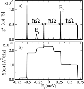
Figure 2: a) Admittance of the driven double quantum dot in a capacitor as a function of the Fermi energy at zero temperature. b) Non-symmetrized current noise power $S(\omega)$ for the same system as a function of the Fermi energy of the external lead. $E_{F}=0$ is the case when the Fermi level matches with the center of the two eigenenergies of the DQD. The parameters in use are $\gamma$=0.16meV, $\Delta_{0}$=0.3meV, $\Delta$=0.4meV, $\Omega$=60.7GHz, $eV_{\Omega}$=0.3meV, and $\omega$=4.55GHz,$V_{0}$=5.1meV, respectively.

We show the admittance of driven double quantum dots in Fig. 2 a). It shows peak structure as a function of Fermi energy. The admittance has peaks when the Fermi energy matches with the resonant energy levels of the DQD as well as photon side bands, $E_{F}\approx E_{r}\pm\hbar\Omega$ where $E_{r}$ is the Floquet eigenvalue of $H_{\Omega}(t)$. For weak driving, $E_{r}$ is the energy eigenvalues for DQD $E_{r}\approx\pm\frac{1}{2}\sqrt{\Delta^{2}+\Delta_{0}^{2}}$. Why does it show peaks? The nonzero admittance of a capacitor is due to the time delay of the electrons at the capacitor. Since only states near the Fermi level are excited by oscillating magnetic flux of low frequency $\omega$, the admittance is naturally given by the Fermi level quantity. So, the peak values of the dwell time at certain Fermi energy give rise to the peak structure of the admittance as clear in Eq.(8). Meanwhile, the role of driving electric field of high frequency $\Omega$ is to help the incoming electron at the Fermi level jump into the resonant levels in double dots via photo absorption or emission. Whenever the Fermi level matches with the resonant energy plus integer multiple of $\hbar\Omega$, the electron can dwell in the dots and the admittance has peaks. This process is depicted in Fig. 3 a).

In Fig. 2 b), we show the noise power as a function of Fermi level. The contribution from equilibrium Nyquist noise is due to electron states near Fermi level. At low frequency and zero temperature, $S_{0}\approx\frac{e^{2}}{4\pi}\omega^{3}\tau_{d}^{2}(E_{F})$buttiker and $S_{P}(\omega)\approx\frac{e^{2}\hbar}{2\pi}\omega^{2}\sum_{m\neq 0}\int d\epsilon|\sum_{l}s^{*}_{l+m}(\epsilon)\frac{d}{d\epsilon}s_{l}(\epsilon+m\hbar\Omega)|^{2}f(\epsilon)(1-f(\epsilon+m\hbar\Omega))$. The sharp peaks in Fig. 2(b) are attributed to the nonzero dwell time at the Fermi levels. In contrast, we find that the non-equilibrium part of noise $S_{P}(\omega)$ shows step-wise behaviour. Why does it show steps? The electrons below Fermi level contribute to the non-equilibrium noise through photon absorption/emission. Note that, in contrast to the case of the admittance, there is no driving probe field of frequency $\omega$. Therefore, the noise power is not necessarily a quantity for the Fermi level. The electrons below Fermi level can contribute to the current fluctuation via photo-assisted tunneling into the dots.

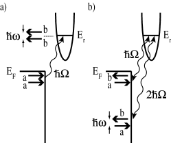
Figure 3: Schematic figures explaining the processes involved in the admittance a) and the current noise b). See the text.

The incoming electron states of energy $E<E_{F}$ contribute to the noise when $E-E_{r}$ is the integer multiple of $\hbar\Omega$. (Fig. 3 b)). Since we consider the current noise power $S(\omega)$ at low frequency $\omega<\Omega$, the outgoing electron states of the energy other than $E+\hbar\omega$ are not involved in the low frequency noise. Therefore, the number of pairs of incoming electron of energy $E$ and the outgoing states of energy $E+\hbar\omega$ determine the strength of the current noise.(Fig. 3 b)). As the Fermi level increases, the number of the pairs increases, which give rise to the step structure. The step arises whenever the Fermi level matches with the resonant energy plus integer multiple of $\hbar\Omega$.

While there have been experimental works on the electrical noise under ac excitation for diffusive conductorsschoelkopf and tunnel junctionsgabelli2 ; deblock , so far there has been no experimental realization of the driven nano-structure tunnel-coupled to single lead. To study the quantum aspect of the admittance discussed in this work, the experimental system by Gabelli et. al.gabelli seems most relevant to the present theoretical work where the dc conductance is zero. For experimental observation of the resonant admittance peaks predicted in this work, the quantum dot in use in Ref.gabelli should be electrically driven and smaller enough to ensure the dot’s quantized energy spacing is larger than the temperature energy scale. To detect the quantum noise at high frequencies, the techniques in Ref.deblock ; onac might be useful where the high frequency noise signal is converted to dc current.

In conclusion, we investigate the low frequency admittance and current noise of nano-structure which is driven by a high frequency field. A fluctuation-dissipation relation for the driven system is obtained. The phase delay time defined through Floquet scattering matrix is essential to understand the admittance. The current noise power shows steps as a function of the Fermi energy when the admittance shows peaks. The Fermionic nature of electrons or the exchange correlation of the incoming electrons is important to the step structure of the noise power.

References

(1) G. Féve et. al.,Science 316, 1169 (2007).
(2) J. Gabelli, et.al., Science 313, 499 (2006).
(3) Ya. M. Blanter and M. Büttiker, Phys. Rep. 336, 1 (2000).
(4)G. B. Lesovik and L. S. Levitov Phys. Rev. Lett. 72,
538(1994).
(5) A. Lamacraft Phys. Rev. Lett. 91, 036804 (2003).
(6) S. Camalet, et.al., Phys. Rev. Lett. 90,
210602 (2003).
(7) M. Büttiker, A. Prêtre,
and H. Thomas, Phys. Rev. Lett. 70, 4114 (1993); M.
Büttiker, H. Thomas, A. Prêtre, Phys. Letters A 180, 364
(1993); A. Prêtre, and H. Thomas, and M. Büttiker, Phys. Rev. B,
54, 8130 (1996).
(8) S. E. Nigg, R. López, and M.
Büttiker, Phys. Rev. Lett. 97, 206804 (2006).
(9) E. P. Wigner, Phys. Rev. 98, 145 (1955);
Felix T. Smith, Phys. Rev. 118, 1 (1960).
(10) G. B. Lesovik and R. Loosen, JETP Lett. 65, 295 (1997).
(11) K.-H. Ahn, H. C. Park, B. Wu, Physica E. 34, 468 (2006); K.-H. Ahn, J. Korean Phys. Soc., 47, 666
(2005).
(12) M. Moskalets and M. Büttiker, Phys.
Rev. B, 66, 205320 (2002).
(13) R. J. Schoelkopf, et. al., Phys. Rev. Lett. 80, 2437
(1998).
(14) J. Gabelli and B. Reulet, Phys. Rev. Lett. 100, 026601 (2008).
(15) R. Deblock, et. al., Science 301,
203 (2003).
(16) E. Onac, et. al., Phys. Rev. Lett. 96, 176601 (2006).