Thermodynamics of vesicle growth and instability

Abstract

We describe the growth of vesicles, due to the accretion of lipid molecules to their surface, in terms of linear irreversible thermodynamics. Our treatment differs from those previously put forward by consistently including the energy of the membrane in the thermodynamic description. We calculate the critical radius at which the spherical vesicle becomes unstable to a change of shape in terms of the parameters of the model. The analysis is carried out both for the case when the increase in volume is due to the absorption of water and when a solute is also absorbed through the walls of the vesicle.

I Introduction

Vesicles are small cell-like structures in which the membrane separating the contents of the vesicle from the environment takes the form of a lipid bilayer. Part of their appeal comes from the fact that living cells are essentially very complex vesicles — with the membrane containing mixtures of different lipids and other components, a cytoskeleton and complex surface structures alb02 . This has led to the use of vesicles as the basic component of models of protocells dea86 ; mor88 ; our99 . On the other hand simple vesicles, without any additional structure, have many fascinating properties when observed in the laboratory. Their self-assembly, their growth, their shape and the fact that they divide to produce daughter vesicles have many aspects which are little-understood. The latter property of replication is especially interesting in the context of models of protocells. One can ask: how much of simple protocell dynamics can be explained using the statistical thermodynamics of vesicles, without the introduction of more complex processes or of genetic material? This question will be the motivation for the present work. In particular we will be interested in describing the dynamics of vesicle growth and the instability which leads to the vesicle changing shape.

To begin the construction of a model for vesicles, it is first necessary to review their dimensions. The typical thickness of the bilayer is $7$nm, while the radius of the vesicle itself can be anything from several times this value up to $100\,\mu$m for so-called giant vesicles. Therefore the bilayer can be thought of as a thin membrane or shell enclosing the contents of the vesicle. In the case of biomolecules the standard picture of this membrane is the fluid mosaic model sin72 where the proteins, enzymes and other such constituents are embedded in the lipid bilayer in which the lipid molecules can freely move as in a liquid. The proteins and enzymes may be able to move from the inner part of the bilayer to the outer part which is in contact with the environment. In the case of interest to us here, these biological aspects are absent and only the fluid nature of the bilayer remains. Therefore the picture which emerges is of a two-dimensional surface, which is supplemented with a thin fluid layer on either side to describe the physical aspect of the bilayer sei97 . Turning this characterization into a quantitative description can be achieved in several different ways; the resulting models go under names such as the spontaneous curvature model hel73 or the bilayer couple model sve82 ; sve83 ; sve89 . However these models have the common feature of a bending energy of the membrane, which is given in terms of the curvature of the two-dimensional surface, together with some extra feature which, in some very basic way, accounts for the fact that the membrane has a thickness. In the spontaneous curvature model this is a extra factor $C_{0}$ subtracted from twice the mean curvature of the surface, and in the bilayer couple model it is a constraint on the mean curvature. Here we will use the spontaneous curvature model, for which the bending energy is $E=(\kappa/2)\int dA\left(2H-C_{0}\right)^{2}$, where $H$ is the local mean curvature, $A$ is the surface area $A$, and $\kappa$ is the bending rigidity.

The vast majority of studies of vesicles based on this form of the bending energy have been of a purely static nature; the energy $E$ has been minimized subject to the constraints that the area of the surface, $A$, and the volume of the vesicle, $V$, are kept constant. The first constraint follows from the large elastic compression modulus; the energy scale associated with this is much greater than that associated with the curvature elasticity and this multiplies a term which fixes $A$ sei97 . Similarly, the energy scale involving the osmotic pressure difference is so large, compared with the curvature energy, that the vesicle volume is effectively fixed. The shapes with the lowest bending energy are usually investigated at different values of a scaled spontaneous curvature and reduced volume. A “phase-diagram” of these minimal shapes in these two variables has quite a complicated structure, with “phases” of prolate ellipsoids, dumb-bell and pear shapes appearing, amongst others sei97 .

Our intention here is to provide a means of linking these snapshots of the vesicle shape. To do this we need a dynamics which gives us a rule to move from one shape to another. We will be chiefly concerned with setting up the correct dynamical description of this system and so we will limit our attention to the growth of spherical vesicles and the transition from a spherical to an ellipsoidal shape. Our treatment differs from the previous studies of this problem boz04 ; boz07 ; mac07a ; mac07b in ways that we describe in detail in Section II. However all these approaches have the common features that they use macroscopic variables and assume that the growth is sufficiently slow that it may be described within the formalism of linear irreversible thermodynamics.

The outline of the paper is as follows. In Section II we introduce the formalism that will be used in the investigation and compare our approach to those used previously. In Section III we carry out the analysis of the growth and loss of stability of the spherical vesicle in the simplest case of a purely aqueous environment and in Section IV we show how this generalizes when a solute is present. In Section V we summarize our results and discuss them in the light of previous work and the model assumptions. There is a mathematical appendix which gives the technical details relating to Sections III and IV.

II Dynamical Description

In the spontaneous curvature model the membrane is a two-dimensional surface, $S$, which separates an inner region, $I$, from the environment, $E$. The outer region could be a purely aqueous environment, or it could also contain a solute, with both the water and solute molecules being able to permeate through the membrane.

The surface is a purely geometric construction; it contains no matter and simply has a bending energy associated with it. If its shape is known, then this bending energy only depends on the volume, $V$, it encloses:

$$E(V)=\frac{\kappa}{2}\oint_{S}\left(C_{1}+C_{2}-C_{0}\right)^{2}\,dA\,,$$ (1)

where $C_{1}$ and $C_{2}$ are the principal radii of curvatures of the surface. In common with the other studies of this system boz04 ; boz07 ; mac07a ; mac07b the deviations from equilibrium will be taken to be sufficiently small that the thermodynamic relation $TdS=dE+P_{i}dV+\sum_{\alpha}\mu_{\alpha}dc_{\alpha}$ can be used. Here $P_{i}$ is the pressure of the fluid inside the membrane, $\mu_{\alpha}$ the chemical potential of chemical $\alpha$ which has concentration $c_{\alpha}$. The only contribution from the membrane is a term $dE=(\partial E/\partial V)dV$, so changing the pressure inside the vesicle from $P_{i}$ to $(P_{i})_{\rm eff}=P_{i}+(\partial E/\partial V)$. Therefore, as long as we replace the internal pressure by this effective pressure, then we may ignore the membrane from a thermodynamic point of view, and simply treat it as a boundary which separates the inside of the vesicle from the environment.

II.1 Purely aqueous environment

The thermodynamic analysis of transport through a membrane which is simply a geometric transition region between two homogeneous regions was carried out by Kedem and Katchalsky fifty years ago ked58 ; ked63 . Suppose, to begin with, that there is no solute present, so that only the flow of water through the membrane need be considered. Then the usual assumption of the thermodynamics of irreversible processes, that the processes under consideration are sufficiently slow to give a linear relation between the fluxes and the forces deG84 , lead to the relation ked58 ; ked63

$$J_{w}=L_{p}\Delta P\,.$$ (2)

Here $J_{w}$ is the flux of water from the environment to the interior, $L_{p}$ is the hydraulic conductivity of the membrane and $\Delta P$ is the difference between the exterior pressure, $P_{e}$, and that of the interior. However, as discussed above, to include the contribution coming from the curvature of the membrane we need to replace $\Delta P$ by the effective pressure difference given by

$$(\Delta P)_{\rm eff}\equiv P_{e}-(P_{i})_{\rm eff}=P_{e}-P_{i}-\left(\frac{\partial E}{\partial V}\right)\equiv\Delta P-\left(\frac{\partial E}{\partial V}\right).$$ (3)

These results may now be brought together. The vesicle is assumed to increase its surface area due to extra lipid molecules being added to the surface. This in turn will change the pressure in the interior, and so change $(\Delta P)_{\rm eff}$ and give rise to a flux of water through the membrane. The rate of increase of the volume of the vesicle will by given by

$$\frac{dV}{dt}=AJ_{w}=L_{p}A\left[\Delta P-\left(\frac{\partial E}{\partial V}\right)\right]\,,$$ (4)

using Eqs. (2) and (3).

We now assume a growth law for the surface area, that is, the rate at which components are incorporated into the vesicle membrane. The simplest, and also the most plausible, is that this is proportional to the surface area boz04 :

$$\frac{dA}{dt}=\lambda A\ \ \Rightarrow\ \ A(t)=A(0)e^{\lambda t}\,.$$ (5)

The analysis below can be carried out with other growth laws. At a more fundamental level we would expect the correct form to emerge from the chemical reactions underlying this process. It is convenient to define a reduced volume by

$$v=\frac{6\pi^{1/2}V}{A^{3/2}}\,,$$ (6)

so that $v=1$ for a sphere and $v<1$ for all other shapes. Then

$$\frac{dv}{dt} = -\frac{3}{2}\lambda v+\frac{6\pi^{1/2}}{A^{3/2}}\frac{dV}{dt}$$ (7)

$$= -\frac{3}{2}\lambda v+\frac{6\pi^{1/2}}{A^{1/2}}L_{p}\left[\Delta P-\left(\frac{\partial E}{\partial V}\right)\right]\,,$$

where we have used Eq. (4).

If the spontaneous curvature, $C_{0}$, was absent in the definition of the bending energy Eq. (1), then the energy would be scale invariant: a typical length scale associated with the vesicle could be changed by an arbitrary scaling factor and $E$ would remain unchanged. However, the inclusion of $C_{0}$, which has dimensions of inverse length, introduces a scale into the problem. Suppose that $R$ is the typical scale factor associated with the vesicle, then scaling the coordinates in Eq. (1) by this factor, the typical length scale associated with the vesicle is unity. After rescaling we denote the principal radii of curvatures by $k_{a}=C_{a}R$, $a=1,2$. Similarly, a dimensionless spontaneous curvature, $k_{0}=C_{0}R$, may be introduced sei97 . If the vesicle is spherical, the typical length scale can be taken to be the radius, and $C_{1}=C_{2}=1/R$. Then

$$E=2\pi\kappa\left(2-C_{0}R\right)^{2}\ \ \Rightarrow\ \ \frac{\partial E}{\partial V}=\frac{C_{0}\kappa}{R^{2}}\left(C_{0}R-2\right)\,.$$ (8)

II.2 Including a Solute

The formalism we have discussed in Section II.1 can be generalized to include a solute. There will now be a flux of solute, $J_{s}$, in addition to the flux of water $J_{w}$, and they will be linearly related to the thermodynamic driving forces which now includes the difference in the osmotic pressure of the solute across the membrane, $\Delta\Pi_{s}$, as well as $\Delta P$ ked58 ; ked63 . The constants multiplying the forces in the linear relations are Onsager coefficients, which will be symmetric in the usual way deG84 . In fact we will use the linear relations involving a slightly different linear combination of variables, corresponding to the “second set of practical phenomenological equations” of Kedem and Katchalsky ked63 :

$$J_{v} = L_{p}\left(\Delta P-\sigma\Delta\Pi_{s}\right)\,,$$ (9)

$$J_{s} = \overline{c}\left(1-\sigma\right)J_{v}+\omega\Delta\Pi_{s}\,,$$ (10)

where $\sigma$ is the reflection coefficient, $\overline{c}$ is the mean concentration of the solute and $\omega$ is the solute permeability. The flux $J_{v}$ is a linear combination of $J_{w}$ and $J_{s}$, namely $J_{v}=J_{w}\overline{V}_{w}+J_{s}\overline{V}_{s}$ where $\overline{V}_{w}$ and $\overline{V}_{s}$ are the partial molar volumes of water and solute respectively. If we assume an ideal solute, then $\Delta\Pi_{s}=k_{B}T\Delta c$ hil86 , where $k_{B}$ is Boltzmann’s constant and $\Delta c$ the difference in concentrations across the membrane. This gives the more useful form

$$J_{v} = L_{p}\left(\Delta P-\sigma k_{B}T\Delta c\right)\,,$$ (11)

$$J_{s} = \overline{c}\left(1-\sigma\right)J_{v}+\omega k_{B}T\Delta c\,,$$ (12)

with $\Delta c=c_{e}-c_{i}$.

In this case the total volume flow per unit area of the membrane is $J_{v}$, and so Eq. (4) is replaced by

$$\frac{dV}{dt}=AJ_{v}=L_{p}A\left[\Delta P-\left(\frac{\partial E}{\partial V}\right)-\sigma k_{B}T\Delta c\right]\,,$$ (13)

where, once again, we have replaced $\Delta P$ by $(\Delta P)_{\rm eff}$ to account for the effect of the membrane curvature. Similarly, if $N$ is the number of molecules of the solute in the interior, then

$$\frac{dN}{dt}=AJ_{s}=A\left[\overline{c}\left(1-\sigma\right)J_{v}+\omega RT\Delta c\right]\,.$$ (14)

This last result may be written in a number of different ways using the relation $N=c_{i}V$.

II.3 Comparisons with Previous Work

The analysis of the growth of vesicles presented in the next section will start from Eqs. (13) and (14). However, we will end this Section by discussing how these two equations differ from those considered by previous workers investigating this problem. In Ref. boz04 it was assumed that no solute was present, so the relevant discussion is that presented in Section II.1. The equation which was used was not Eq. (4), however, since the term involving the bending energy was introduced in a very different way: the pressure difference in Eq. (2) was simply set equal to $(\partial E/\partial V)$, resulting in the pressure difference being completely absent from Eq. (4). We believe our approach to be the correct way of proceeding. The method of Ref. boz04 is extended to include a solute in Ref. boz07 . A further point of disagreement with our treatment is that the reflection coefficient, $\sigma$, is set equal to unity. However this is only true if the membrane is impermeable to the solute, in which case $\omega$ should equal zero too. The simultaneous use of Eq. (13) and Eq. (14) when $\sigma=1$ was already argued against in the original paper of Kedem and Katchalsky ked58 .

The work reported in Refs. mac07a and mac07b has a different philosophy; there it is assumed that the instability by which the division process begins — the sphere becomes unstable to an ellipsoid — is a Turing instability. Thus these authors introduce spatial effects, and the boundary of a two-dimensional vesicle is defined on a lattice. The “total pressure” involving the sum of the hydrostatic pressure difference, the osmotic pressure difference and the term coming from the surface energy are all included. However, since this is a two-dimensional vesicle, the form of the bending energy is different, and it is not clear to us why the surface tension is included with such a large modulus. Thermodynamic relations similar to Eqs. (13) and (14) are used, but apparently not to directly describe the change in vesicle shape. It is also not so clear to us what role the two metabolic centers that these authors introduce have in giving an initial anisotropy to the vesicle and how crucial they are in initiating the symmetry-breaking instability. Clearly subsequent divisions will produce vesicles without these centers and therefore the mechanism will have to still work in their absence.

One of the goals of the present work is to clarify the various assumptions made and systematize the methodology that is used to study vesicle growth and division.

III The first bifurcation

In the purely static analysis of the model defined by Eq. (1), it is known that when the sphere becomes unstable, the stable shape which replaces it is the ellipsoid sei91 . As an initial application of the formalism of Section II, we will investigate this instability from a dynamical viewpoint when no solute is present.

The axisymmetric ellipsoid will be parametrized by expressing the Cartesian coordinates as

$$x = a\sin\theta\cos\phi\,,$$

$$y = a\sin\theta\sin\phi\,,$$

$$x = c\cos\theta\,,$$ (15)

where $0\leq\phi<2\pi$, $-\pi/2<\theta<\pi/2$ and where $a$ and $c$ are constants. For a sphere $a=c\equiv R$, the radius. If the ellipsoid only differs in shape from the sphere very slightly, then $a$ and $c$ may be expressed as

$$a=R\left(1+a_{1}\epsilon\right)\,,\ \ c=R\left(1+c_{1}\epsilon\right)\,,$$ (16)

where $\epsilon$ is a small quantity and $a_{1}$ and $c_{1}$ are numbers which characterize the shape of the ellipsoid; if $a_{1}>c_{1}$ it is oblate and if $a_{1}<c_{1}$ it is prolate.

Using standard results bey87 and (16), it is straightforward to calculate the surface area and volume of the ellipsoid for small $\epsilon$. The details are given in the Appendix where it is shown that

$$A = 4\pi R^{2}\left[1+\frac{2}{3}\left(2a_{1}+c_{1}\right)\epsilon+{\cal O}\left(\epsilon^{2}\right)\right]\,,$$

$$V = \frac{4}{3}\pi R^{3}\left[1+\left(2a_{1}+c_{1}\right)\epsilon+{\cal O}\left(\epsilon^{2}\right)\right]\,.$$ (17)

From these expressions we see immediately that the reduced volume, $v$, defined by Eq. (6) is $1+{\cal O}(\epsilon^{2})$, and so we have to go to next order in Eq. (17) to find the deviation of the reduced volume from the value $1$ which it has when the vesicle is spherical. From Eqs. (43) and (44) we see that

$$v=1-\frac{4}{15}\left(a_{1}-c_{1}\right)^{2}\epsilon^{2}+{\cal O}\left(\epsilon^{3}\right)\,,$$ (18)

with $v<1$ for all cases except the sphere ($a_{1}=c_{1}$) as required. The bending energy is also straightforward to calculate, but much more tedious. From it we can determine $\partial E/\partial V$, as described in the Appendix.

Substituting the expressions for $v$ and $\partial E/\partial V$ into Eq. (7) we find

$$\frac{8}{15\,\ln 2}\left(a_{1}-c_{1}\right)^{2}\epsilon\frac{d\epsilon}{d\tau}=F_{0}+F_{1}\epsilon+F_{2}\epsilon^{2}+{\cal O}\left(\epsilon^{3}\right)\,,$$ (19)

where the $F_{j}$ ($j=0,1,2$) are functions of $R,\Delta P,C_{0}$ and $\eta(\equiv L_{p}\kappa C^{4}_{0}\ln 2/\lambda)$ and are given explicitly in Eq. (53). We have also introduced a scaled time $\tau=t/T_{d}$, where $T_{d}=\ln 2/\lambda$ is the time taken for the surface area to double in value. For Eq. (19) to be consistent as $\epsilon\to 0$ we require $F_{0}=0$, which gives $\Delta P$ in terms of $R,C_{0}$ and $\eta$:

$$\frac{\Delta P}{\kappa}=\frac{C_{0}^{4}R\ln 2}{2\eta}+\frac{C_{0}^{2}}{R}-\frac{2C_{0}}{R^{2}}\,.$$ (20)

Since Eq. (20) holds as $\epsilon\to 0$, it is true for the sphere and could have been obtained more directly from the bending energy of a spherical vesicle given in Eq. (8). Then, since for a sphere

$$\frac{dV}{dt}=\frac{R}{2}\frac{dA}{dt}=\frac{\lambda R}{2}A\,,$$

we see from Eq. (4) that

$$\frac{\lambda R}{2}=L_{p}\left[\Delta P-\frac{\kappa C_{0}R(C_{0}R-2)}{R^{3}}\right]\,,$$ (21)

which agrees with Eq. (20). The quantity $\Delta P$ is the pressure difference required for the vesicle to remain a sphere while growing at a steady rate given by $\lambda$.

Setting $F_{0}=0$ in Eq. (19), one sees that the two sides of the equation are not of the same order as $\epsilon\to 0$ unless $F_{1}=0$. From the explicit form for this function given in the Appendix, setting $\Delta P$ equal to the value given in Eq. (20) gives the result displayed in Eq. (54). We see that, apart from making a particular choice for $R$ in terms of $C_{0}$ and $\eta$, we can only make $F_{1}$ equal to zero by taking $(2a_{1}+c_{1})=0$. This simply amounts to a particular choice of ellipsoid shape. It is, in some sense, the most symmetrical choice and consists of changes in the direction of the two symmetric axes being half of that in the third direction (and having the opposite sign).

Finally, setting both $F_{0}$ and $F_{1}$ equal to zero, which implies the choice Eq. (20) and $c_{1}=-2a_{1}$, gives the expression (56) for $F_{2}$ and leads to

$$\frac{d\epsilon}{d\tau}=\left(\frac{13\eta}{8C^{2}_{0}R^{2}}-\frac{9\eta}{2C^{3}_{0}R^{3}}-\frac{13\ln 2}{16}\right)\epsilon+{\cal O}\left(\epsilon^{2}\right)\,.$$ (22)

If the term on the right-hand side of this equation is positive, then the sphere will be unstable to a transformation into an ellipsoid. This is the case if $2\eta(13C_{0}R-36)>13C_{0}^{3}R^{3}\ln 2$, which can never be satisfied if $C_{0}R<36/13$. Similarly when viewed as an inequality which is cubic in $C_{0}R$, one finds that it cannot be satisfied for any real positive $C_{0}R$ if $\eta<\eta_{\rm min}$ where

$$\eta_{\rm min}=\frac{3^{7}\,2\ln 2}{13^{2}}\approx 17.94\,.$$ (23)

For $C_{0}R>36/13$ the condition for the sphere to be unstable may be written as

$$\eta>\frac{1}{2}\left(\frac{13C_{0}^{3}R^{3}\ln 2}{13C_{0}R-36}\right)\,.$$ (24)

The region of instability is shown in Fig. 1. For values of $\eta>\eta_{\rm min}$ a dynamical transition can eventually occur, the vesicle turning into an ellipsoid. We are only interested in the first transition which is encountered as $R$ increases, which occurs for values of $C_{0}R$ greater than $36/13$, but less than the value that corresponds to $\eta=\eta_{\rm min}$. This latter condition gives the result $C_{0}R=54/13$. Therefore the critical radius, $R_{c}$, at which the transition occurs, lies in the range $36/13<C_{0}R_{c}<54/13$. It is interesting to note the fundamental role that the phenomenological factor $C_{0}$ has in determining the critical radius.

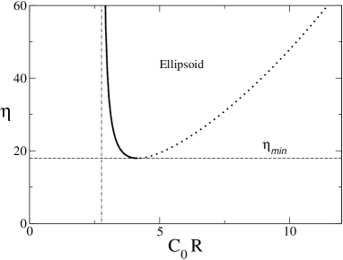
Figure 1: The transition line defining the region of instability in the parameter plane ($C_{0}R$, $\eta$) is depicted for a purely aqueous environment. There is no transition below the horizontal dashed line (which represents $\eta_{\rm min}=17.94$) and to the left of the vertical dashed-dotted line (which represents $C_{0}R=36/13$). In the remaining portion of the figure, the thick solid line represents the transition from the region on the left where the spherical configuration is dynamically favored, to the region on the right, where the ellipsoid configuration is dynamically favored. The dotted line is an unphysical solution of the cubic equation (26).

So, in summary, we suppose that initially the vesicle is a sphere of radius $R(0)$. It then grows according to Eq. (5), that is, the radius increases according to $R(t)=R(0)e^{\lambda t/2}$. The pressure difference between the interior of the vesicle and the exterior during this growth phase may be found from Eq. (20) to be

$$\frac{\Delta P}{\kappa}=\frac{C^{4}_{0}R(0)\ln 2}{2\eta}e^{\lambda t/2}+\frac{C^{2}_{0}}{R(0)}e^{-\lambda t/2}-\frac{2C_{0}}{R(0)^{2}}e^{-\lambda t}\,.$$ (25)

The growth phase continues until the vesicle has achieved a radius of $R_{c}$, which is the smallest real positive root of the cubic equation found by setting $F_{2}$ equal to zero:

$$13C_{0}^{3}R_{c}^{3}\ln 2-26\eta C_{0}R_{c}+72\eta=0\,.$$ (26)

As discussed above there are no such roots for $\eta<\eta_{\rm min}$, given by Eq. (23), and for $\eta>\eta_{\rm min}$, $C_{0}R_{c}$ has to lie in the narrow range $[2.77,4.15]$. The critical radius is reached at a time

$$t_{c}=\frac{2}{\lambda}\ln\left(\frac{R_{c}}{R(0)}\right)\ \ {\rm or}\ \ \tau_{c}=\frac{\ln\left(R_{c}/R(0)\right)^{2}}{\ln 2}\,.$$ (27)

At this time the spherical shape becomes unstable and the vesicle takes on an ellipsoidal shape.

IV The bifurcation with a solute present

In Section II we developed the formalism for the situation where a solute was present, but for simplicity the analysis of Section III assumed that the solute was absent. In this Section we will repeat the analysis of Section III with the solute included.

The extra term which appears in Eq. (13) which changes the position of the instability is $-\sigma k_{B}T\Delta c$. To calculate it we need to determine $\Delta c$. This can be found from the other equation we introduced, Eq. (14), however an integral over time has to be performed. To see this, we use Eq. (13) to write Eq. (14) as

$$\frac{d\left(c_{i}V\right)}{dt}=\overline{c}\left(1-\sigma\right)\frac{dV}{dt}+A\,\omega k_{B}T\Delta c\,,$$ (28)

where $\overline{c}=\Delta c/\ln(c_{e}/c_{i})$ ked58 . If we know $A$ and $V$ as functions of $t$, then we can in principle solve this differential equation for $c_{i}(t)$ and so find $\Delta c(t)$, which can then be substituted into Eq. (13).

To illustrate these basic ideas, we will consider the special case where the membrane is impermeable to solute molecules, so that the number of solute molecules, $N$, is constant. However $c_{i}(t)$ does change with time, due to the fact that the volume, $V$, increases with time, and this has a non-trivial effect on the instability analysis. A membrane impermeable to solute molecules is defined by $\sigma=1$ and $\omega=0$. It follows directly from Eq. (28) that $c_{i}V$ is a constant, and so

$$c_{i}(t)=\frac{c_{i}(0)V(0)}{V(t)}\,.$$ (29)

Then the term $-k_{B}T\Delta c$ which appears in Eq. (13) gives rise to an additional term on the right-hand side of Eq. (7) which equals

$$-\frac{6\pi^{1/2}}{A^{1/2}V}L_{p}k_{B}T\left\{c_{e}V(t)-c_{i}(0)V(0)\right\}\,.$$ (30)

Using the expressions (17), this becomes

$$- \frac{3L_{p}k_{B}T}{R^{4}}\left\{1-\frac{4}{3}\left(2a_{1}+c_{1}\right)\epsilon+{\cal O}\left(\epsilon^{2}\right)\right\}$$

$$\times \left\{c_{e}R^{3}\left[1+\left(2a_{1}+c_{1}\right)\epsilon+{\cal O}\left(\epsilon^{2}\right)\right]-c_{i}(0)R^{3}(0)\right\}\,,$$

to first order in $\epsilon$, since initially the vesicle is a sphere.

To see how these changes affect Eq. (19) let us write it as

$$\frac{8}{15\,\ln 2}\left(a_{1}-c_{1}\right)^{2}\epsilon\frac{d\epsilon}{d\tau}=G_{0}+G_{1}\epsilon+G_{2}\epsilon^{2}+{\cal O}\left(\epsilon^{3}\right)\,,$$ (32)

where the $G_{j}$ ($j=0,1$) are related to the $F_{j}$ as follows:

$$G_{0} = F_{0}-\frac{3\eta\Phi\left[3\Gamma-4\pi R^{3}c_{e}\right]}{4\pi C^{4}_{0}R^{4}\ln 2}$$ (33)

$$G_{1} = F_{1}+\frac{\eta\Phi\left[3\Gamma-\pi R^{3}c_{e}\right]}{\pi C^{4}_{0}R^{4}\ln 2}\,,$$ (34)

where $\Gamma=c_{i}(0)V(0)$ and $\Phi=\sigma k_{B}T$. The analogous result for $G_{2}$ is given by Eq. (LABEL:G_2) in the Appendix. Following the same line of argument as in Section III we require $G_{0}$ and $G_{1}$ to be zero in order for the stability analysis to be applicable. The first condition gives an expression for the pressure difference across the membrane:

$$\frac{\Delta P}{\kappa} = \frac{C_{0}^{4}R\ln 2}{2\eta}+\frac{C_{0}^{2}}{R}-\frac{2C_{0}}{R^{2}}$$ (35)

$$+ \frac{\sigma k_{B}T}{R^{3}}\left(R^{3}c_{e}-R^{3}(0)c_{i}(0)\right)\,,$$

which shows the additional terms that are added to Eq. (20) when a solute is present. The second condition, $G_{1}=0$ again implies that $(2a_{1}+c_{1})=0$ and so the addition of the solute does not change the shape of the ellipsoid for which the stability analysis applies.

If we now use the conditions found by implementing $G_{0}=0$ and $G_{1}=0$ in Eq. (LABEL:G_2) and substituting this into Eq. (32) we find

$$\frac{d\epsilon}{d\tau} = \left(\frac{13\eta}{8C^{2}_{0}R^{2}}-\frac{9\eta}{2C^{3}_{0}R^{3}}-\frac{13\ln 2}{16}\right.$$ (36)

$$- \left.\frac{45\Gamma\Phi\eta}{32\pi C^{4}_{0}R^{4}}\right)\epsilon+{\cal O}\left(\epsilon^{2}\right)\,,$$

which gives the required modification of Eq. (22). A similar analysis to that given in Section III shows that if $4\pi C_{0}R(13C_{0}R-36)<45\Gamma\Phi$, then the sphere is always stable, no matter what the value of $\eta$. This gives the minimum value of the radius, $R$, which can lead to an instability (corresponding to an infinite value for $\eta$) to be

$$C_{0}R_{\rm min}=\frac{18}{13}\left[1+\sqrt{1+\frac{65\Gamma\Phi}{144\pi}}\right]\,.$$ (37)

If $R>R_{\rm min}$, the spherical shape is unstable if

$$\eta>\left(\frac{26\pi C_{0}^{4}R^{4}\ln 2}{4\pi C_{0}R\left(13C_{0}R-36\right)-45\Gamma\Phi}\right)\,.$$ (38)

Figure 2 depicts the domain of instability in the parameter plane $(C_{0}R,\eta)$. Different curves refer to different choices of the quantity $\Gamma\Phi$, and allow the qualitative inspection of the modification induced by the presence of a solute. The condition for a double root of the quartic equation for $C_{0}R$ gives, as in Section III, the maximum value of $R$ which can lead to an instability:

$$C_{0}R_{\rm max}=\frac{27}{13}\left[1+\sqrt{1+\frac{65\Gamma\Phi}{162\pi}}\right]\,.$$ (39)

with the corresponding value of $\eta$ being $\eta_{\rm min}$. This can be determined as a function of $\Gamma\Phi$ by substituting the expression (39) for $C_{0}R_{\rm max}$ back into the quartic equation. The resulting function is shown as an inset in Fig. 2. This increases as $\Gamma\Phi$ increases (larger solute concentration and/or higher temperature). However, the ratio of $R_{\rm max}/R_{\rm min}$ remains essentially unchanged at about $1.5$ for all values of $\Gamma\Phi$. This means that the range of values of the radius at which the spherical shape becomes unstable remains quite small.

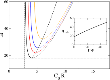
Figure 2: (Color online) The region of instability is depicted for the case when a solute is included in a similar manner to that shown in Fig. 1 when a solute is not present. Different curves refer to distinct values of the product $\Gamma\Phi$ (= 0, 5, 10, 20). The dotted line which passes through the minima of these curves shows the maximum value of $C_{0}R$ for which a transition can occur, and is given by Eq. (39). The corresponding value of $\eta$, $\eta_{\rm min}$, is plotted in the inset as a function of the quantity $\Gamma\Phi$.

V Conclusion

Despite the great interest in the growth, change in shape and division of vesicles, very little is known about the nature of the processes that govern them. Even fundamental questions about the typical vesicle radii at the various stages or the hydrostatic or osmotic pressure differences between the exterior and interior, are still largely open. The main obstacle to achieving a greater understanding is the difficulty in carrying out experiments. Even qualitatively, a consistent picture is hard to achieve, and so a theoretical description which would help with the interpretation of experimental results would be very welcome. In this paper we have proposed such a description, taking extra care to correctly incorporate the energy associated with the curvature of the membrane in the thermodynamic description. We have concentrated on establishing the formalism and demonstrating it on the initial stages of the growth and on the first bifurcation to an ellipsoid. The subsequent time evolution of the vesicle, leading to division, can now be investigated, but this can only be carried out numerically and we leave it for the future.

The vesicle growth is ultimately caused by the incorporation of lipids from the environment into the vesicle wall. This will increase the area, which in turn will lead to a change in the internal hydrostatic pressure and so initiate a flow of fluid through the membrane. This will happen extremely slowly — at a rate governed by the parameter $\lambda$, and so in practice the vesicle will never become flaccid and will maintain a spherical shape in the initial stages of the evolution. It is the quasi-static nature of the expansion that allows us to use the formalism of linear irreversible thermodynamics deG84 . This predicts, among other things, that the radius of the vesicle will grow according to $R(t)=R(0)e^{\lambda t/2}=2^{t/(2T_{d})}$ using $\lambda=\ln 2/T_{d}$. However this exponential growth gets cut off at a radius, $R_{c}$, given by the smallest real solution of Eq. (26) at a critical time given by Eq. (27). This critical radius falls into a remarkably narrow range. The corresponding value of the hydrostatic pressure can then be determined.

It is interesting to compare these results with those found by the previous studies discussed in Section II.3. In Refs. boz04 ; boz07 , the term involving the bending energy on the right of Eq. (4) was effectively omitted and therefore the expression (20) did not contain the final two terms, which originate from this term (see Eq. (8)). It could be argued that it is a legitimate approximation, in the sense that for the parameters of interest, this term is negligible compared to the one that is retained. Since we have included both contributions, we are able to test this by calculating the ratio between the first term on the right-hand side of Eq. (20) and the sum of the second and third terms. We find that this ratio always lies between $0$ and $1$. That is, the terms omitted in Refs. boz04 ; boz07 are always more important than the one included. This ratio is actually zero at one extreme of the range of allowed values of $R$ ($C_{0}R=36/13$, which corresponds to an infinite value of the parameter $\eta$), and increases monotonically to $9/14$ when $C_{0}R$ takes on its greatest allowed value ($54/13$) and $\eta$ takes on its smallest allowed value ($17.94$). It should also be remarked that in Ref.  boz04 the value of $\eta$ used is $1.85$, which is the value at which vesicle splitting gives rise to two equal vesicles, which are equal in size to the initial vesicle. Given the inconsistencies in the formulation we have just alluded to, it is doubtful that this value is correct. Further work is required to enable a comparison between the work reported in Refs. mac07a and mac07b and our approach. As explained in Section II.3, the method used is very different: the vesicle is a closed curve in two dimensions, metabolic centers are present which induce the symmetry breaking and the results obtained are purely numerical.

These results, and others involving the nature of the initial bifurcation, provide an initial set of predictions which can be compared with future experiments. Of course, the model as it stands is quite simple and many features could be made more realistic. For instance, $C_{0}$ is almost certainly not a constant, and becomes non-zero during the course of the vesicle growth. Nevertheless, taking a non-zero $C_{0}$ induces a transition polm . Another aspect that we have not included in the present treatment is a discussion of the effect of thermal fluctuations on the shape of the vesicle. At first sight it is not obvious if thermal fluctuations will have any appreciable effect. An order of magnitude calculation wor97 suggests that under most circumstances fluctuations will not need to be taken into account, however near an instability there may be a significant effect. Within the static picture, which has been the subject of by far the majority of papers to date, the procedure for investigating the effect of thermal fluctuations is clear hel84 ; sei94 ; hei97 ; wor97 ; far03 . The shape is written as a sum of a stationary term plus a small fluctuation and the energy expanded to quadratic order in the fluctuation. Putting this into a Boltzmann factor, the Gaussian integrals may be performed. However there are a number of technical issues, such as the inclusion of constraints. There is also the question of the size of non-Gaussian fluctuations. Nevertheless, it is clear that thermal fluctuations can shift the position of an instability, or even change its nature completely. The analogous calculation carried out within the present framework would be even more complex, however it should definitely be addressed in future work.

Despite such shortcomings, and there are undoubtedly others, we believe that the model is sufficiently detailed to provide a reasonably good description of vesicle growth and hope that it will serve to clarify a number of aspects in this fascinating, and neglected, field.

Appendix A Surface area, volume and bending energy of an ellipsoid

In this Appendix we will collect together the results which are required to calculate the reduced volume and the bending energy of an ellipsoid in Section III, together with the generalization in Section IV.

The ellipsoids we consider here are axisymmetric. The prolate version is formed by rotating an ellipse with semi-minor axis $a$ and semi-major axis $c$ (i.e. $c>a$) about the major axis. It surface area is given by bey87

$$A=2\pi a^{2}+\frac{2\pi ac^{2}}{\sqrt{c^{2}-a^{2}}}\sin^{-1}\left[\frac{\sqrt{c^{2}-a^{2}}}{c}\right]\,.$$ (40)

For an oblate ellipsoid, $c<a$, and bey87 ,

$$A=2\pi a^{2}+\frac{\pi ac^{2}}{\sqrt{a^{2}-c^{2}}}\ln\left[\frac{a+\sqrt{a^{2}-c^{2}}}{a-\sqrt{a^{2}-c^{2}}}\right]\,.$$ (41)

In both cases their volume is given by bey87

$$V=\frac{4}{3}\pi a^{2}c\,.$$ (42)

Substituting the parametrizations (16) into the expressions (40)-(42) one finds Eq. (17). As mentioned in the text, this immediately implies that the reduced volume is 1 to this order, and so we have to go to next order in $\epsilon$ to see some deviation from the result for a sphere. At next order

$$A = 4\pi R^{2}\left[1+\frac{2}{3}\left(2a_{1}+c_{1}\right)\epsilon\right.$$ (43)

$$+ \left.\frac{1}{15}\left(6a_{1}^{2}+c_{1}^{2}+8a_{1}c_{1}\right)\epsilon^{2}+{\cal O}\left(\epsilon^{3}\right)\right]\,,$$

and

$$V = \frac{4}{3}\pi R^{3}\left[1+\left(2a_{1}+c_{1}\right)\epsilon\right.$$ (44)

$$+ \left.\left(a^{2}_{1}+2a_{1}c_{1}\right)\epsilon^{2}+{\cal O}\left(\epsilon^{3}\right)\right]\,,$$

which together give the expression (18) for $v$ to second order in $\epsilon$.

The other quantity we have to evaluate is the bending energy, $E$, given by Eq. (1). This involves evaluating the two integrals

$$J_{1}\equiv\oint_{S}H\,dA\,,\ \ J_{2}\equiv\oint_{S}H^{2}\,dA\,,$$ (45)

where $H=(C_{1}+C_{2})/2$ is the mean curvature. For an axisymmetric ellipsoid this is given by bey87

$$H=\frac{c\left[3a^{2}+c^{2}+\left(a^{2}-c^{2}\right)\cos 2\theta\right]}{\left[a^{2}\cos^{2}\theta+c^{2}\sin^{2}\theta\right]^{3/2}}\,.$$ (46)

Evaluating the integrals in Eq. (45) using the result (46) yields

$$J_{1} = 2\pi c+\frac{\pi a^{2}}{\sqrt{c^{2}-a^{2}}}\ln\left[\frac{c+\sqrt{c^{2}-a^{2}}}{c-\sqrt{c^{2}-a^{2}}}\right]\ \ (c>a)\,,$$

$$J_{1} = 2\pi c+\frac{2\pi a^{2}}{\sqrt{a^{2}-c^{2}}}\sin^{-1}\left[\frac{\sqrt{a^{2}-c^{2}}}{a}\right]\ \ (c<a)\,,$$

and

$$J_{2} = \frac{\pi c^{2}}{a}\left\{\frac{\sin^{-1}\left[\frac{\sqrt{c^{2}-a^{2}}}{c}\right]}{\sqrt{c^{2}-a^{2}}}+\frac{7a}{3c^{2}}-\frac{2a^{3}}{3c^{4}}\right\}\ \ (c>a)\,,$$

$$J_{2} = \frac{\pi c^{2}}{a}\left\{\frac{{\rm tanh}^{-1}\left[\frac{\sqrt{a^{2}-c^{2}}}{a}\right]}{\sqrt{a^{2}-c^{2}}}+\frac{7a}{3c^{2}}-\frac{2a^{3}}{3c^{4}}\right\}\ \ (c<a)\,.$$

Substituting the parametrizations (16) into the expressions (LABEL:J_1s) and (LABEL:J_2s), and using Eq. (43), one obtains

$$E = 2\pi\kappa\left\{\left(C_{0}R-2\right)^{2}+\frac{2}{3}\left(2a_{1}+c_{1}\right)C_{0}R\left(C_{0}R-2\right)\epsilon\right.$$

$$+ \frac{1}{15}\left[c_{1}^{2}\left(32-4C_{0}R+C^{2}_{0}R^{2}\right)+8a_{1}c_{1}\left(-8+C_{0}R\right.\right.$$

$$+ \left.\left.\left.C_{0}^{2}R^{2}\right)+a_{1}^{2}\left(32-4C_{0}R+6C_{0}^{2}R^{2}\right)\right]\epsilon^{2}+{\cal O}\left(\epsilon^{3}\right)\right\}\,.$$

The aim is to calculate $\partial E/\partial V$ which we achieve by using

$$\frac{\partial E}{\partial V}=\frac{\partial E}{\partial R}\frac{dR}{dV}\,.$$ (50)

From Eq. (LABEL:ener_second) one finds

$$\frac{\partial E}{\partial R} = 4\pi\kappa C_{0}\left\{\left(C_{0}R-2\right)+\frac{2}{3}\left(2a_{1}+c_{1}\right)\left(C_{0}R-1\right)\epsilon\right.$$ (51)

$$+ \frac{1}{15}\left[c_{1}^{2}\left(C_{0}R-2\right)+4a_{1}c_{1}\left(1+2C_{0}R\right)\right.$$

$$+ \left.\left.a_{1}^{2}\left(6C_{0}R-2\right)\right]\epsilon^{2}+{\cal O}\left(\epsilon^{3}\right)\right\}\,,$$

and from Eq. (44)

$$\frac{dV}{dR} = 4\pi R^{2}\left[1+\left(2a_{1}+c_{1}\right)\epsilon\right.$$ (52)

$$+ \left.\left(a^{2}_{1}+2a_{1}c_{1}\right)\epsilon^{2}+{\cal O}\left(\epsilon^{3}\right)\right]\,,$$

which gives an expression for $\partial E/\partial V$. Substituting this into Eq. (7), and making use of the expression (18) for $v$ we obtain Eq. (19) with the $F_{j}$ ($j=0,1,2$) given by

$$F_{0} = 3\left(\frac{C_{0}^{4}R^{3}\ln 2-4C_{0}\eta+2C_{0}^{2}\eta R-2\Delta\tilde{P}\eta R^{2}}{2C_{0}^{4}R^{3}\ln 2}\right)\,,$$

$$F_{1} = \left(2a_{1}+c_{1}\right)\eta\left(\frac{6C_{0}-2C_{0}^{2}R+\Delta\tilde{P}R^{2}}{C_{0}^{4}R^{3}\ln 2}\right)\,,$$

$$F_{2} = \frac{1}{15C_{0}^{4}R^{3}\ln 2}\left[2a_{1}c_{1}(-82C_{0}\eta+16C_{0}^{2}\eta R\right.$$ (53)

$$- 9\Delta\tilde{P}\eta R^{2}+6C_{0}^{4}R^{3}\ln 2)-c_{1}^{2}(98C_{0}\eta-29C_{0}^{2}\eta R$$

$$+ 6\Delta\tilde{P}\eta R^{2}+6C_{0}^{4}R^{3}\ln 2)-a_{1}^{2}(278C_{0}\eta$$

$$- \left.74C_{0}^{2}\eta R+21\Delta\tilde{P}\eta R^{2}+6C_{0}^{4}R^{3}\ln 2)\right]\,,$$

where $\Delta\tilde{P}=\Delta P/\kappa$.

As explained in the main text, setting $F_{0}=0$ gives Eq. (20). Using this expression for $\Delta P$ then gives

$$F_{1}=\left(2a_{1}+c_{1}\right)\left(\frac{C^{3}_{0}R^{3}\ln 2+8\eta-2\eta C_{0}R}{C_{0}^{3}R^{3}\ln 2}\right)\,.$$ (54)

Apart from exceptional values of $R$, this vanishes only when $2a_{1}+c_{1}=0$.

If we now set $c_{1}=-2a_{1}$ we find from Eq. (53) that

$$F_{2}=3a_{1}^{2}\left(\frac{14C_{0}^{2}\eta R-38C_{0}\eta-\Delta\tilde{P}\eta R^{2}-6C_{0}^{4}R^{3}\ln 2}{5C_{0}^{4}R^{3}\ln 2}\right)\,.$$ (55)

Finally, setting $\Delta P$ to the value given in Eq. (20) one finds

$$F_{2}=3a_{1}^{2}\left(\frac{26\eta C_{0}R-13C_{0}^{3}R^{3}\ln 2-72\eta}{10C_{0}^{3}R^{3}\ln 2}\right)\,,$$ (56)

which leads to Eq. (22).

In Section IV, the calculation is carried out in the present of a solute. The equation which describes the instability is now Eq. (32) with $G_{0}$ and $G_{1}$ given by Eqs. (33) and (34) respectively and $G_{2}$ given by

$$G_{2} = F_{2}-\frac{\eta\Phi}{10\pi C^{4}_{0}R^{4}\ln 2}\left[4a_{1}c_{1}\left(21\Gamma-3\pi R^{3}c_{e}\right)\right.$$

$$+ \left.c^{2}_{1}\left(33\Gamma-4\pi R^{3}c_{e}\right)+2a^{2}_{1}\left(54\Gamma-7\pi R^{3}c_{e}\right)\right]\,,$$

where once again $\Gamma=c_{i}(0)V(0)$ and $\Phi=\sigma k_{B}T$.

References

- (1) B. Alberts et al. Molecular Biology of the Cell, (Garland Science, New York, 2002). Fourth edition.
- (2) D. W. Deamer. Orig. Life Evol. Biosph. 17, 3 (1986).
- (3) H. J. Morowitz, B. Heinz, and D. W. Deamer. Orig. Life Evol. Biosph. 18, 281 (1988).
- (4) G. Ourisson and Y. Nakatani. Tetrahedron 55, 3183 (1999).
- (5) S. I. Singer and G. L. Nicholson. Science 175, 720 (1972).
- (6) U. Seifert. Adv. Phys. 46, 13 (1997).
- (7) W. Helfrich. Z. Naturforsch. C28, 693 (1973).
- (8) S. Svetina, A. Ottova-Leitmanova, and R. Glaser. J. Theor. Biol. 94, 13 (1982).
- (9) S. Svetina and B. Z̆eks̆. Biochem. Biophys. Acta 42, 86 (1983).
- (10) S. Svetina and Z̆eks̆. Eur. Biophys. J 17. 101 (1989).
- (11) B. Boz̆ic̆ and S. Svetina. Eur. Biophys. J. 33, 565 (2004).
- (12) B. Boz̆ic̆ and S. Svetina. Eur. Phys. J. E24, 79 (2007).
- (13) J. Macia and R. V. Solé. J. Theor. Biol. 245, 400 (2007).
- (14) J. Macia and R. V. Solé. Phil. Trans. R. Soc. 362, 1821 (2007).
- (15) O. Kedem and A. Katchalsky. Biochim. Biophys. Acta 27, 229 (1958).
- (16) O. Kedem and A. Katchalsky. Trans. Faraday Soc. 59, 1918 (1963).
- (17) S. R. de Groot and P. Mazur. Non-Equilibrium Thermodynamics (Dover, New York, 1984).
- (18) T. L. Hill. An Introduction to Statistical Thermodynamics (Dover, New York, 1986).
- (19) U. Seifert, K. Berndl and R. Lipowsky. Phys. Rev. A44, 1182 (1991).
- (20) W. H. Beyer. CRC Standard Mathematical Tables (CRC Press, Baton Rouge, 1987).
- (21) P. Olmsted (private communication).
- (22) M. Wortis, M. Jarić and U. Seifert. Jour. Mol. Liq. 71, 195 (1997).
- (23) W. Helfrich and R-M. Servuss. Il Nuovo Cimento 3D, 137 (1984).
- (24) U. Seifert. Z. Phys. B97, 299 (1995).
- (25) V. Heinrich, F. Sevs̆ek, S. Svetina and B. Z̆eks̆. Phys. Rev. E 55, 1809 (1997).
- (26) O. Farago and P. Pincus. Eur. Phys. J. E11, 399 (2003).