TeV variability in blazars: how fast can it be?

Abstract

Recent Cerenkov observations of the two BL Lac objects PKS 2155–304 and Mkn 501 revealed TeV flux variability by a factor $\sim$ 2 in just 3–5 minutes. Even accounting for the effects of relativistic beaming, such short timescales are challenging simple and conventional emitting models, and call for alternative ideas. We explore the possibility that extremely fast variable emission might be produced by particles streaming at ultra–relativistic speeds along magnetic field lines and inverse Compton scattering any radiation field already present. This would produce extremely collimated beams of TeV photons. While the probability for the line of sight to be within such a narrow cone of emission would be negligibly small, one would expect that the process is not confined to a single site, but can take place in many very localised regions, along almost straight magnetic lines. A possible astrophysical setting realising these conditions is magneto–centrifugal acceleration of beams of particles. In this scenario, the variability timescale would not be related to the physical dimension of the emitting volume, but might be determined by either the typical duration of the process responsible for the production of these high energy particle beams or by the coherence length of the magnetic field. It is predicted that even faster TeV variability – with no X–ray counterpart – should be observed by the foreseen more sensitive Cerenkov telescopes.

1 Introduction

In the standard framework, the overall non-thermal energy distribution of blazars is produced within a relativistic jet closely aligned to the line of sight. While the origin of the flux variability is not known, for a variability timescales $t_{\rm var}$ the general causality argument imposes the limit $R\lower 3.22916pt\hbox{$\sim$}\hbox to0.0pt{\hss\raise 1.1625pt\hbox{$<$}}ct_{\rm var}\delta$ on the typical dimension $R$ of a quasi–spherical emitting region, where $\delta$ is the Doppler factor of the radiating plasma. This constrain can be bypassed if the dimension of the region along the line of sight is much smaller than the other two dimensions. Such a configuration is the natural one arising in shocks forming within the flow (internal shock model, Spada et al. 2001, Guetta et al. 2004). In this scenario the minimum variability timescale is related to the Schwarzschild radius $R_{\rm s}$ of the central black hole, $t_{\rm var}>R_{\rm s}/c$, due to the cancellation of the bulk Lorentz factors.

Unprecedented ultra–fast variability at TeV energies has been recently detected from the blazars Mkn 501 (Albert et al. 2007) and PKS 2155–304 (Aharonian et al. 2007), on timescales as short as $t_{\rm var}\sim$ 3–5 minutes. And in the latter source (at $z=0.116$) the variable high energy radiation corresponded to an observed (isotropic) luminosity $L\sim 10^{47}$ erg s^-1, which was dominating the broadband emission.

As pointed out by Begelman, Fabian & Rees (2008) – the observations of ultra–fast variability strongly challenges the above framework in both geometrical configurations. In the case of a quasi–spherical region, the short variability timescale implies that the source is too compact (see Begelman et al. 2008) unless extreme values for $\delta$ ($>100$) are assumed, at odds with – among other beaming indicators – the relatively low velocity estimated for the knots in their pc–scale jets (Piner et al. 2008; but see Ghisellini et al. 2005 for a possible solution). In the internal shock scenario, $t_{\rm var}$ is totally inconsistent with the typical black hole masses hosted in blazar nuclei.

In principle there is no lower limit on the dimension of an emitting region and thus variability timescales could be decoupled from the typical minimum scale of the system: the average emission, typically varying on timescales $t_{\rm var}\sim 10^{4}$ s, could still be produced over volumes comparable to the jet size, while sporadic, ultra–fast flares could originate in very localised regions. However, as the flux of the ultra–fast flares was comparable to the bolometric one, a further condition would have to occur (such as an extremely efficient radiation mechanism, a high Lorentz factor for the emitting plasma, a particular geometry). It is thus meaningful to wonder whether there is any robust physical limit to the observed duration and luminosity of flares.

In this work we tackle this question in the context of leptonic emission models, i.e. the observed high energy radiation is produced, via inverse Compton, by relativistic leptons. We first consider a completely ideal case which maximises the effects of relativistic beaming showing that, under particular conditions involving beams of highly relativistic emitting particles, no observationally interesting limit holds. Then the astrophysical feasibility of such an ideal case is examined, and we propose a more specific setting which seems an ideal environment to produce such narrow beams.

2 An idealised limit to fast TeV variability

Relativistic amplification of the emitted radiation is the key physical process on which the standard model for blazars is based. Typically it is postulated that high–energy electrons ($\gamma>10^{5}$) move with random directions within the emitting region which, in turn, is propagating with a bulk Lorentz factor of $\Gamma\sim 10$ at a small angle with respect to the line of sight.

However, if the highly relativistic electrons were almost co–aligned in a narrow beam (as considered by, e.g., Aharonian et al. 2002, Krawczynski 2008) we can achieve a more efficient situation – in terms of detected emission – for observers aligned with the beam. Before assessing the physical feasibility of such a configuration let us consider the consequences on the observed emission.

The energy loss for (standard) inverse Compton (IC) scattering of an electron with Lorentz factor $\gamma=(1-\beta^{2})^{-1/2}$ embedded in a radiation field of energy density $U_{\rm r}$ is (e.g. Rybicki & Lightman 1979):

$$P\,=\,\dot{\gamma}m_{\rm e}c^{2}\,=\,{4\over 3}\sigma_{\rm T}c\gamma^{2}U_{\rm r},$$ (1)

where $\sigma_{\rm T}$ is the Thomson cross section and the seed photon field is assumed isotropically distributed. In Eq. 1 $P$ represents the power emitted by the electrons, while the power received by an observer depends on the viewing angle: within the cone $1/\gamma$ time is Doppler contracted by the factor $(1-\beta)$ and the isotropic equivalent power $P_{\rm iso}$ is enhanced by the factor $(1-\beta)^{-1}$, as the radiation is collimated in a solid angle $\Delta\Omega=2\pi(1-\beta)$. The two effects combine to yield a maximum observed power

$$P_{\rm iso,max}\,=(1-\beta)^{-2}P\,=(1+\beta)^{2}\gamma^{4}P\sim{16\over 3}\sigma_{\rm T}c\gamma^{6}U_{\rm r}.$$ (2)

If the electron and the observer remain ”aligned” for a time longer than the radiative cooling time $t_{\rm c}$, radiation will be seen for

$$t_{\rm r}\,=(1-\beta)t_{\rm c}\,=\,{3m_{\rm e}c\over 4\sigma_{\rm T}(1+\beta)\gamma^{3}U_{\rm r}}.$$ (3)

Let us estimate how many electrons $N$ are required in order to observe $P_{\rm iso,max}\sim 10^{47}L_{47}$ erg s^-1 in the TeV range. For simplicity we first consider the case where the source has no bulk motion and the seed photons are isotropically distributed. This requires $\gamma\geq 10^{6}$, in order to produce TeV photons. Then

$$N\,=\,{10^{47}L_{47}\over P_{\rm iso,max}}\,=\,9.4\times 10^{59}\,{L_{47}\over\gamma^{6}U_{\rm r}}=\,9.4\times 10^{23}\,{L_{47}\over\gamma^{6}_{6}U_{\rm r}},$$ (4)

corresponding to a mass $Nm_{\rm e}\sim 0.85L_{47}/(\gamma^{6}_{6}U_{\rm r})$ milligrams and an energy $E=\gamma Nm_{\rm e}c^{2}=7.7\times 10^{23}L_{47}/(\gamma^{5}_{6}U_{\rm r})$ erg.

Emission would be observed for a mere $t_{\rm r}\,=1.5\times 10^{-11}/(\gamma_{6}^{3}U_{\rm r})$ s, during which an electron would travel for a cooling distance $\Delta R_{\rm c}=\beta ct_{\rm c}=9\times 10^{11}$ cm towards the observer.

This idealised limit to the shortest time variability observable in the TeV range, even thought unrealistic, shows that high amplitude, apparent luminosity variability is physically possible even over sub–nanosecond timescales.

In the sketched scenario the variability timescales – unrelated to the size of the emitting region – may reflect how long a beam maintains its coherence and alignment with the observer’s line of sight, and/or the duration of the process responsible to produce such a beam.

2.1 Energy requirements

The first issue to be discussed in relation to the idealised case concerns the feasibility of attaining realistic configurations which allow this “streaming scenario” without requiring a large amount of energy.

If electrons stream along magnetic field lines, the latter should maintain their direction (within a factor $1/\gamma$) for a minimum scale length, of the order of the electron cooling one ($\sim\Delta R_{c}\sim 10^{11}-10^{12}$ cm). This probably imposes the most severe constrain, but it is hard to meaningfully quantify it. If electrons move along non–parallel (or partly curved) magnetic field lines, at any given time the probability of observing radiation (from electrons pointing along the line of sight) increases. On the other hand, this of course requires more electrons (to account for those not emitting towards the observer at a given instant).

For a flare during which the observed luminosity $L$ doubles in a time $\Delta t$, the numbers and total energy of electrons required to radiate the observed average $L$ are a factor $\Delta t/t_{\rm r}$ larger than what just derived above. As an illustrative example, the TeV flare of PKS 2155–304 lasted for $\Delta t=100\Delta t_{2}$ s, yielding $\Delta t/t_{\rm r}=6.7\times 10^{12}\Delta t_{2}\gamma_{6}^{3}U_{\rm r}$. It follows that the total energy which has to be invoked to sustain the observed average $L=10^{47}L_{47}$ erg s^-1 for $\Delta t$ is

$$E\,=\,\gamma Nm_{\rm e}c^{2}{\Delta t\over t_{\rm r}}\,=\,5.2\times 10^{36}\,{L_{47}\Delta t_{2}\over\gamma^{2}_{6}}\quad{\rm erg}.$$ (5)

Note that $E$ is independent of $U_{\rm r}$ (as expected, since only electron energies are involved). The term $\gamma^{-2}$ enters through the solid angle of the beamed radiation.

The inferred energetics would be not particularly demanding, but it corresponds to a single particle beam. As the probability that such a beam is oriented along the line of sight with an accuracy of order $1/\gamma$ is exceedingly small, the existence of many beams along field lines, whose directions cover a sizeable fraction $f$ of the jet opening angle $\theta_{\rm j}$, is mandatory for the process to be of any astrophysical relevance.

If $A$ is the number beams – each subtending a solid angle $\Delta\Omega_{\rm b}=2\pi[1-\cos(1/\gamma)]$ – with directions within the jet solid angle $\Delta\Omega_{\rm j}=2\pi(1-\cos\theta_{\rm j})$,

$$f\,\approx\,A\,{\Delta\Omega_{\rm b}\over\Delta\Omega_{\rm j}}\,\sim\,{A\over(\gamma\theta_{\rm j})^{2}}\,\sim\,10^{-10}\,{A\over(\gamma_{6}\theta_{\rm j,-1})^{2}}.$$ (6)

$f$ can be in principle roughly estimated by the “duty cycle” of the high energy ultra–fast flares, namely the fraction of the observational time during which flares are visible. Therefore, if one ultra–fast flare is detected during an observing time interval $T_{\rm obs}$,

$$f\,=\,{\Delta t\over T_{\rm obs}}\,=\,10^{-3}\,{\Delta t_{2}\over T_{\rm obs,5}}\,\to\,A\,\sim 10^{7}\,(\gamma_{6}\theta_{\rm j,-1})^{2}\,{\Delta t_{2}\over T_{\rm obs,5}}$$ (7)

where $T_{\rm obs}\sim 10^{5}$ s has been assumed (likely a lower limit).

Consequently the total energetics, $E_{\rm tot}$, which also accounts for beams not pointing at the observer amounts to

$$E_{\rm tot}\,=\,AE\,=\,5.2\times 10^{43}\,{\Delta t_{2}\over T_{\rm obs,5}}\,L_{47}\Delta t_{2}(\theta_{\rm j,-1})^{2}\quad{\rm erg}$$ (8)

independently of $\gamma$. This corresponds to the bulk energy of leptons responsible of flares. Modelling of the average spectral energy distribution of TeV blazars, and in particular of PKS 2155–304 (see e.g. Foschini et al. 2007; Celotti & Ghisellini 2007; Ghisellini & Tavecchio 2008) imply jet powers of the order $L_{\rm jet}\sim 10^{45}$ erg s^-1, largely exceeding $E_{\rm tot}/\Delta t$. We conclude that from the energetics point of view, the proposed mechanism is not demanding.

2.2 Partial isotropization of pitch angles and synchrotron emission

The mechanism responsible for the acceleration of particles along field lines could in principle favour a distribution of pitch angles $\psi$ peaked at small values, of the order $\sim 1/\gamma$ (see Section 3).

It is also likely though that small disturbances in the field configuration result in values $\psi$ greater than $1/\gamma$. The solid angle of emission is then $\Delta\Omega_{\rm b}=2\pi(\psi/\gamma)\gg\pi/\gamma^{2}$: the IC power emitted by the beam will spread over a larger solid angle (implying a reduced observed flux), but this effect will be compensated by photons emitted along the line of sight from other beams.

When the electrons acquire a non–vanishing pitch angle $\psi$, they also emit synchrotron radiation. It is interesting to evaluate the corresponding flux. Like the IC radiation, the synchrotron power $P_{\rm s,iso}$, received by an “aligned” observer, is amplified by a factor $(1-\beta\cos\psi)^{-1}$ with respect to the emitted one, $P_{\rm s,e}$. The radiation is collimated within a solid angle of the order $\Delta\Omega_{\rm s}\sim 2\pi\sin\psi/\gamma$,

$$P_{\rm s,iso}\, = \,P_{\rm s,e}\,\,{4\pi\gamma\over 2\pi\sin\psi}\,\,{1\over 1-\beta\cos\psi}$$ (9)

$$= \,4\sigma_{\rm T}cU_{B}\gamma^{3}\beta^{2}{\sin\psi\over 1-\beta\cos\psi}$$

This is maximised at $\sin\psi=1/\gamma$ at a value

$$P_{\rm s,iso,max}\,=\,4\sigma_{\rm T}cU_{B}\gamma^{4}\beta^{2},\quad(\sin\psi=1/\gamma),$$ (10)

which is a factor $2\gamma^{2}$ larger than for an electron with pitch angle $\psi=90^{\circ}$. With respect to Eq. 2, the ratio of observed and emitted power is smaller by a factor $\gamma^{2}$, as synchrotron emission has an extra pitch–angle dependence ($\propto 1/\gamma^{2}$ for $\psi\sim 1/\gamma$).

To summarise. Only IC radiation (and no synchrotron) is observed from leptons perfectly aligned with the magnetic field lines, and in turn with the observer. For pitch angles of the order $1/\gamma$, the synchrotron flux received from a single electron is maximised, yet the ratio of the received powers (IC/synchrotron) is a factor $\sim\gamma^{2}$ larger (cfr Eq. 2 with Eq. 10) than the corresponding ratio in the isotropic pitch angle case. In other words, radiation from streaming electrons will produce effects more pronounced in the IC than in the synchrotron branch of the spectral distribution.

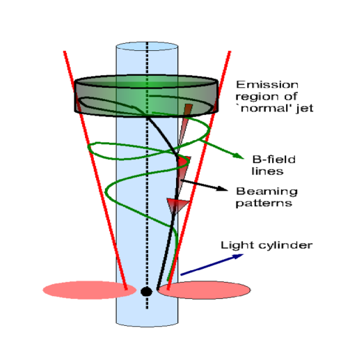
Figure 1: Schematic representation of the proposed scenario. At some distance from the black hole and accretion disc part of the jet power is dissipated in a region moving with a bulk Lorentz factor 10–30, producing radiation through “standard” synchrotron and self–Compton emission. Magneto–centrifugally accelerated electrons are bound to stream along magnetic field lines, initially oriented with different directions. They would reach the light cylinder at different locations where the electrons reach their maximum energy. Beyond the light cylinder field lines wound–up since they cannot move rigidly any longer. Occasionally, magnetic field lines close to the light cylinder would point towards the observer. In these cases one can then detect the relativistically boosted radiation resulting from the IC scattering by the magneto–centrifugally accelerated electrons off the seed photons produced by the “normal” jet and/or by the accretion flow.

3 A possible astrophysical setting: magneto–centrifugal acceleration

A natural astrophysical mechanism producing a configuration similar to the one proposed, where highly relativistic electrons stream along magnetic field lines, is centrifugal acceleration (e.g. Rieger & Mannheim 2000, Osmanov et al. 2007, Rieger & Aharonian 2008).

Several models invoking centrifugal acceleration assume that magnetic field lines rigidly rotate at a fraction of the black hole rotational velocity. A charged test particle, injected at the base and co–rotating with the field (as “bead–on–wire”) will experience the centrifugal force and will be accelerated with an efficiency that increases as the particle approaches the light cylinder (Machabeli & Rogava 1994; Machabeli et al. 1996; Gangadhara & Lesch 1997; Rieger & Mannheim 2000; Osmanov et al. 2007). The energy boost will be limited by radiative losses due to IC process and/or by the breakdown of the “bead–on–wire” approximation, when the Coriolis force – tearing the particle off the field line – exceeds the Lorentz force. The effective limiting mechanism depends on the accretion disc luminosity: the former (latter) will dominate for higher (lower) radiation energy densities. Maximum electron Lorentz factors around $\gamma=10^{8}$ can be attained under reasonable conditions when, as in TeV emitting BL Lacs, the accretion disc is radiatively very inefficient (Osmanov et al. 2007). If, besides the accretion disc, there are other sources of cooling photons, the maximum $\gamma$ will be smaller. In TeV BL Lacs the radiation produced by the “normal” jet region can in some cases dominate (but not by a huge factor) the cooling. We have checked that in such conditions the maximum $\gamma$–factor reaches values as large as $10^{6}$, as required to produce TeV radiation. Protons suffer less from radiative losses and their maximum energy is limited by the breakdown of the “bead–on–wire” approximation. As a result, protons and electrons can achieve comparable energies in such a case.

Before and during the acceleration three important effects will concur to decrease the final electron pitch angle:

1. the magneto–centrifugal force increases only the parallel component of the particle momentum;

2. the magnetic field decreases with distance: therefore the pitch angle of the accelerated electron will also decrease, as in a magnetic bottle;

3. at the beginning of the acceleration, the electron is likely sub–relativistic due to strong radiation losses since close to the accretion disc the radiation and magnetic fields are most intense (see below).

In the following we examine these effects in some details: Magneto–centrifugal acceleration – The force vector can be decomposed into two components, parallel and perpendicular to the magnetic field line. During a gyro–orbit, the perpendicular one acts half of the time in favour and half against the electron motion, with a null average effect. Only the parallel momentum of the particle will then be increased in the process. Adiabatic invariant – Since the electron moves along divergent magnetic field lines, its pitch angle will decrease. A simple estimate can be made using the adiabatic invariant in the form

$${(p^{\prime}_{\perp})^{2}\over B^{\prime}}\,=\,{\rm constant}\,\to p^{\prime}_{\perp}\,\propto\,(B^{\prime})^{1/2},$$ (11)

where $p^{\prime}_{\perp}\equiv\gamma^{\prime}_{\perp}\beta^{\prime}_{\perp}$ is the dimensionless transverse electron momentum in the gyro–frame. A Lorentz transformation in the lab frame yields:

$$\gamma\,=\,\gamma_{\parallel}\gamma^{\prime}_{\perp},\qquad\beta_{\perp}\,=\,{\beta^{\prime}_{\perp}\over\gamma_{\parallel}},$$ (12)

from which

$$\tan\psi\,=\,{\beta_{\perp}\over\beta_{\parallel}}\,\to\,\sin\psi\,={p^{\prime}_{\perp}\over\gamma\beta}.$$ (13)

As $p^{\prime}_{\perp}$ will decrease owed to the decrease of the $B$–field (Eq. 11) while $\gamma$ will increase thanks to acceleration, the pitch angle will decrease. Thus even though initially an electron is mildly relativistic in the gyro–frame (i.e. $p^{\prime}_{\perp}\lower 3.22916pt\hbox{$\sim$}\hbox to0.0pt{\hss\raise 1.1625pt\hbox{$>$}}1$) this ensures that the final pitch angle is of the order of $1/\gamma$. Radiative cooling – For an electron with initial large pitch angle and large $p^{\prime}_{\perp}$ the decreasing magnetic field might not be sufficient to yield a final small $\psi$. However, close to the accretion disk, the magnetic field is large, implying severe radiation losses. While synchrotron losses do not affect the pitch angle (synchrotron photons radiated by a relativistic electron are emitted along the electron velocity direction), they limit $p^{\prime}_{\perp}$ (e.g. $p^{\prime}_{\perp}$ reaches trans–relativistic values for $B\sim 100$ G at a scale of $R\sim 10^{15}$ cm). A similar effect is produced by IC scattering, as in the electron rest frame virtually all seed photons are seen as coming from the forward direction and the scattering cross section is azimuthally symmetric (both in the Thomson and in the Klein Nishina regime).

3.1 The spectrum: qualitative considerations

The equilibrium distribution of particles, solution of the kinetic equation including the acceleration and cooling terms, can be described by a power–law with typical slope $N(\gamma)\propto\gamma^{-n}$, with $n=3/2$ (Rieger & Aharonian 2008). For an isotropic pitch angle distribution the corresponding IC spectrum is of the form $\propto\nu^{-(n-1)/2}\propto\nu^{-1/4}$ (if the seed photons are monochromatic and their energy density is constant along the electron beam). If the seed photons are distributed as $F(\nu_{\rm s})\propto\nu_{\rm s}^{-\alpha_{s}}$, with $\alpha_{s}>1/4$, the slope of the scattered spectrum is the same of the slope of the seeds, i.e. $\alpha_{s}>1/4$, and somewhat steeper at high frequencies if Klein–Nishina effects are important. This is the limit when there is a large ensemble of beams covering a wide range of directions.

The other limit is when only the radiation from a single beam can be observed. This comprises particles with a range of $\gamma$ and, correspondingly, of pitch angles (cfr Eq. 13): lower energy electrons, predominant at the start of the acceleration process, will have the largest pitch angles; the most energetic electrons, with the smallest pitch angles, will tend to be located at the end of the accelerating zone and will mostly contribute to the emission in the TeV band.

The observed spectral slope of the radiation from a single beam can be qualitatively estimated for a beam along a (straight) field line perfectly aligned with the line of sight, and a particle energy power–law distribution $N(\gamma)\propto\gamma^{-n}$.

Let us discuss first the case of monochromatic seed photons, of frequency $\nu_{0}$. The up–scattered photons will have an average frequency $\nu\propto\gamma^{2}\nu_{0}$ for scatterings in the Thomson regime, and $\nu\propto\gamma$ in the Klein–Nishina one.

If the energy density of the seeds are roughly the same for electrons of low and high $\gamma$, the resulting spectral slope will correspond to

$$L(\nu)\propto N(\gamma)P_{\rm iso,max}{d\gamma\over d\nu} \propto \nu^{(5-n)/2}\,\quad{\rm Thomson}$$ (14)

$$\propto \nu^{(6-n)}\qquad{\rm Klein~{}Nishina},$$

as $P_{\rm iso,max}\propto\gamma^{6}$ for a single electron (Eq. 2). As above, if the seed photons are distributed as $F(\nu_{\rm s})\propto\nu_{\rm s}^{-\alpha_{s}}$ the slope of the scattered spectrum is the same of the slope of the seeds, and somewhat steeper at high frequencies if Klein–Nishina effects are important.

The observed spectral slope will depend on the distributions of the emitting beams. In any case, at TeV energies, we expect a slope very similar to the slope of the seed photon distribution, steepening at the highest frequencies because of Klein–Nishina effects.

As for the seed photons, we will have always at least two components: the radiation coming from the (inefficient) accretion flow (see Mahadevan 1997 for illustrative examples of disc spectra) and the radiation produced by the “normal” active region of the jet. Their relative importance depends on their luminosities and spectra, the distance of the electron beams, and the bulk velocity of the active region of the jet. For typical values (i.e. disc luminosities $\sim 10^{41}$ erg s^-1, jet comoving luminosities $\sim 10^{43}$ erg s^-1, and beams located at $\sim 10^{17}$ cm from a disc of size $\sim 10^{16}$ cm) the jet radiation dominates. In this case the spectrum produced by the electron beam is expected to be very similar to the SSC spectrum of the jet.

4 Discussion and observational tests

We have suggested that ultra–fast TeV variability could originate from particles “streaming” along magnetic field lines, namely beams of highly relativistic electrons with very small pitch angles that occasionally point towards the observer, giving rise to flare events.

These leptons could inverse Compton scatter synchrotron photons produced by the population of electrons responsible for the broad band radiation detected most of the observing time, characterised by variability timescales of a few hours. The latter, “normal” jet emission also comprises a synchrotron self–Compton TeV component, expected to vary coherently with the synchrotron one at X–rays frequencies.

Usually, the streaming particles would point in directions off the line of sight, but changes in the magnetic lines orientation result in a non zero probability that they become closely aligned with it. The probability for this to occur depends on the geometry, the degree of coherence of the magnetic field and the total number of particle beams (pointing in any direction). The latter number can be estimated from the (admittedly still poorly determined) duty cycle of the ultra–fast variability events: the required total energy is not demanding.

Within this scenario there is in principle no astrophysical interesting limit on how fast TeV variability can be. Variations the order of $10^{47}$ erg s^-1 in the apparent luminosity can occur even over sub–nanosecond timescales. However a typical minimum variability timescale could be estimated for a specific geometrical setting. For illustration, consider a configuration where magnetic field lines, before reaching the light cylinder, rigidly rotate at some velocity $\beta_{\rm B}c$ and the emission region is located at some distance $z$ from the black hole. Particles travelling along a given field line with pitch angle $\sim 1/\gamma$, will emit in a particular direction for a time:

$$t_{\rm var}\,=\,{2\over\gamma}\,{2\pi\theta_{\rm j}z\over\beta_{\rm B}c}\,\sim\,0.5\,{\theta_{\rm j,-1}z_{\rm 16}\over\beta_{\rm B}\gamma_{6}}\,\,{\rm s},$$ (15)

where $2\pi\theta_{\rm j}z/\beta_{\rm B}c$ is the rotational period of the field line and $2/\gamma$ is the fraction of the rotational period during which the beaming cone subtends the line of sight. Thus in this geometrical situation the minimum variability timescale is expected to be of the order of a second. This simply refers to a single field line, aligned (within a factor $1/\gamma$) for at least one cooling length (i.e. for $\sim 10^{12}$ cm) – if this is not the case $t_{\rm var}$ would be shorter. It also assumes a single bunch of electrons whose emission can be observed: $t_{\rm var}$ would be longer if we can detect the radiation from particles streaming on other adjacent field lines.

The variability timescale of these ultra–fast events is not related to the typical dimension of the emitting region and depends on the duration of the acceleration phase and on the time interval over which the magnetic field lines are aligned with the line of sight.

Magneto–centrifugal acceleration scenario can easily produce beams of electrons with pitch angles of the order $1/\gamma$. This can be achieved if initially (i.e. at the base of the jet) the particles are not relativistic, as indeed radiation losses ensure.

The general scenario where “needle beams” of very energetic electrons with small pitch angles can account for ultra–fast TeV variability bear some relevant consequences that can be observationally tested:

• Although in principle TeV variability timescales could be extremely short, in the proposed astrophysical setting a typical minimum value can be of the order of a second (Eq. 15). As a consequence, more and more sensitive Cerenkov telescopes and arrays should detect faster and faster flux variability. Peak fluxes need not to be smaller for shorter events.

• No correlation between X–ray and TeV flux is expected during ultra–fast flares, as synchrotron emission from the streaming particles is weaker than the inverse Compton one by a factor $\gamma^{2}$. Ultra–fast TeV variability should resemble the phenomenology of “orphan flares” (as detected from the TeV BL Lac 1959+650; Krawczynski et al. 2004). On the contrary, the synchrotron and inverse Compton fluxes produced by the normal jet should vary in a correlated way. Furthermore the normal jet synchrotron flux is likely to always dominate over the streaming particle synchrotron component and thus no ultra–fast events should be observed in the X–ray band.

• Variability should be faster at higher inverse Compton frequencies, as they are produced by the higher energy electrons which also have the smallest pitch angles. This also implies that the observed flux has to be produced by a smaller number of streaming particle bunches, namely higher energy flares should be rarer.

• TeV spectra, during ultra–fast variability, are expected to be similar to less active phases, as observed in the flaring state of PKS 2155–304 (Aharonian et al. 2007).

References

- (1) Aharonian F., Akhperjanian A.G., Razer–Bachi A.R. et al., 2007, ApJ, 664, L71
- (2) Aharonian F., Timokhin A.N. & Plyasheshnikov A.V., 2002, A&A, 384, 834
- (3) Albert J., Aliu E., Anderhub H. et al., 2007, ApJ, 669, 862
- (4) Begelman M.C., Fabian A.C. & Rees M.J., 2008, MNRAS, 384, L19
- (5) Foschini L., Ghisellini G., Tavecchio F. et al., 2007, ApJ, 657, L81
- (6) Gangadhara R.T., & Lesch H. 1997, A&A, 323, L45
- (7) Ghisellini G., Tavecchio F. & Chiaberge M., 2005, A&A, 432, 401
- (8) Guetta D., Ghisellini G., Lazzati D. & Celotti A., 2004, A&A, 421, 877
- (9) Krawczynski H., 2008, ApJ, 659, 1063
- (10) Krawczynski H., Hughes S.B., Horan D. et al., 2004, ApJ, 601, 151
- (11) Machabeli G.Z. & Rogava A.D., 1994, Ph. Rv. A., 50, 98
- (12) Machabeli G.Z., Nanobashvili I.S. & Rogava A.D.. 1996, Radiophysics and Quantum Electronics, 39, 26
- (13) Machabeli G.Z., Osmanov Z.N. & Mahajan S.M., 2005, PhPL, 12, 2901
- (14) Mahadevan R., 1997, ApJ, 477, 585
- (15) Osmanov Z., Rogava A. & Bodo G., 2007m A&A, 470, 395
- (16) Piner G.B., Pant N. & Edwards P.G., 2008, ApJ, 678, 64
- (17) Rieger F.M. & Aharonian F., 2008, A&A, 479, L5
- (18) Rieger F.M. & Mannheim K., 2000, A&A, 353, 473
- (19) Rybicki G.B. & Lightman A.P., 1979, Radiation processes in astrophysics, Wiley & Sons (New York)
- (20) Spada M., Ghisellini G., Lazzati D. & Celotti A., 2001, MNRAS, 325, 1559