Resolution of the Distance Ambiguity for Galactic H II Regions

Abstract

We resolve the kinematic distance ambiguity for 266 inner Galaxy H ii regions out of a sample of 291 using existing H i and ${}^{13}{\rm CO}$ sky surveys. Our sample contains all H ii regions with measured radio recombination line (RRL) emission over the extent of the ${}^{13}{\rm CO}$ Boston University—Five College Radio Astronomy Observatory Galactic Ring Survey ($18\arcdeg\ <l<55\arcdeg$ and $|b|<1$) and contains ultra compact, compact, and diffuse H ii regions. We use two methods for resolving the distance ambiguity for each H ii region: H i emission/absorption (H i E/A) and H i self-absorption (H i SA). We find that the H i E/A and H i SA methods can resolve the distance ambiguity for 72% and 87% of our sample, respectively. When projected onto the Galactic plane, this large sample appears to reveal aspects of Galactic structure, with spiral arm-like features at Galactocentric radii of 4.5 and 6 kpc, and a lack of H ii regions within 3.5 kpc of the Galactic center. Our H ii regions are approximately in the ratio of 2 to 1 for far verses near distances. The ratio of far to near distances for ultra-compact H ii regions is 2.2 to 1. Compact H ii regions are preferentially at the near distance; their ratio of far to near distances is 1.6 to 1. Diffuse H ii regions are preferentially at the far distance; their ratio of far to near distances is 3.8 to 1. This implies that the distinction between ultra compact and compact H ii regions is due largely to distance, and that the large angular size of diffuse H ii regions is not due solely to proximity to the Sun.

1 INTRODUCTION

H ii regions are the clearest tracers of massive star formation because of their visibility across the Galactic disk at cm-wavelengths. Without a known distance, however, the physical properties of H ii regions remain unknown. Distances allow one to transform measured properties such as flux and angular size into physical properties such as luminosity and physical size. The knowledge of these properties for H ii regions is vital to understanding the process of star formation in our Galaxy.

The simplest and most common way to estimate the distance to an H ii region with a measured velocity is to assume a Galactic rotation curve. Rotation curves generally model axially symmetric circular orbits such that a source’s velocity is a function only of Galactocentric distance. There have been many models of Galactic rotation proposed using various tracers (e.g Burton & Gordon 1978; Clemens 1985; Brand 1986; Fich, Blitz & Stark 1989; McClure-Griffiths & Dickey 2007). All rotation curves have some amount of intrinsic error because they are simplified models of a more complicated rotation pattern. Additionally, when transforming velocities into distances, velocities that depart from circular rotation (due to streaming motions) will cause errors in the derived distance. Streaming motions result in velocity deviations of $\sim 10$ $\,{\rm km\,s}^{-1}$ (Burton 1971; Stark & Brand 1989), which cause a distance uncertainty up to 2 kpc over the longitude range of our present study.

While the procedure of transforming velocities into distances is straightforward in the outer Galaxy, most distances in the inner Galaxy are degenerate: for each velocity there are two possible distances. These two distances (a “near” and a “far” distance) are spaced equally about the tangent point distance. This problem has become known as the kinematic distance ambiguity (KDA). For only one positive velocity along each line of sight, the tangent point velocity, is the degeneracy not present. Determining whether the H ii regions in our sample lie at the near or the far distance is the goal of this paper.

One method that has proved effective at resolving the KDA towards H ii regions is H i Emission/Absorption, hereafter H i E/A. All H ii regions emit broadband thermal free-free continuum radiation in the cm-wavelength regime. Neutral H i gas between the H ii region and the observer will absorb the thermal continuum if the brightness temperature of the H i is less than that of the H ii region at 21 cm. Because the continuum emission is broadband, and not limited to a particular frequency (velocity), all foreground H i has the potential to absorb the H ii region’s continuum. In the first quadrant, the LSR velocity increases with distance from the Sun, reaches a peak at the tangent point, and decreases with distance thereafter (see Figure 1). Thus H ii regions at the near distance will show H i absorption lines from foreground clouds at velocities up to their radio recombination line (RRL) velocity. If an H ii region is at the far distance, it will show absorption from foreground H i clouds with velocities up to the tangent point velocity. The H i E/A method therefore relies on H i absorption at velocities between the RRL and tangent point velocity to distinguish between the near and the far distance.

Many authors have used H i E/A to resolve the KDA for H ii regions. Kuchar & Bania (1994) used both pointed Arecibo 21 cm H i observations (HPBW of $4\arcmin$) and also Boston University—Arecibo Observatory Galactic H i Survey data (hereafter BUAO H i survey; Kuchar & Bania 1993) to resolve the KDA for 70 Galactic H ii regions. Fish et al. (2003) resolved the KDA using the H i E/A method for a sample of 20 UC H ii regions using the VLA in A- or BnA-configurations ($1\arcsec$ to $6\arcsec$ synthesized beam). Kolpak et al. (2003) measured the 21 cm H i absorption spectrum towards 49 H ii regions using the VLA in C-configuration ($16\arcsec$ synthesized beam). The high success rate of these efforts proves the utility of H i E/A experiments in H ii region distance determinations.

A second method that has been used to resolve the KDA is H i self-absorption, hereafter H i SA. H i SA is useful for resolving the KDA for molecular clouds. Cold foreground H i will absorb against warmer background H i at the same velocity. Liszt, Burton & Bania (1981) hypothesized that Galactic molecular clouds must contain residual H i, a result that has been confirmed by many observations (e.g. Wannier et al. 1991; Kuchar & Bania 1993; Williams & Maddalena 1996). The H i gas associated with molecular clouds is cold ($\sim 10\,{\rm K}$) compared the the warm H i in the ISM ($\sim 100\,{\rm K}$). The H i inside a molecular cloud at the near distance will absorb against the warm background H i at the same LSR velocity that lies at the far distance. The H i inside a molecular cloud at the far distance shows no such absorption as there is no background H i at the same velocity. Thus the signature of a cloud at the near distance is molecular emission at the same velocity and with the same line width as an H i absorption feature. Since H ii regions are almost always associated with molecular gas (Anderson et al. 2008; hereafter Paper I), the distance to H ii regions can be found using H i SA.

Molecular clouds frequently display H i SA features (e.g. Knapp 1974). A theoretical study by Flynn et al. (2004) showed that all model molecular clouds could produce H i SA. Jackson et al. (2002) found a strong H i SA signal associated with the molecular cloud located at ($l,b$)=($45\fdg 6,+0\fdg 3$) using the BUAO H i survey (Kuchar & Bania 1993) and the BU–FCRAO ${}^{13}{\rm CO}$  Galactic Ring Survey data (GRS; Jackson et al. 2006). Goldsmith & Li (2005) found that the ${}^{13}{\rm CO}$ molecule is a very good tracer of H i SA. More recently, Busfield et al. (2006) used H i SA analysis to determine the distances towards massive young stellar object candidates.

One can also use formaldehyde (${\rm H_{2}CO}$) absorption to resolve the KDA. This method is identical to the H i E/A method, except that the absorber is ${\rm H_{2}CO}$ instead of H i. Again, it is the broadband nature of the radio continuum emission of H ii regions that makes this method possible, as the radio continuum and ${\rm H_{2}CO}$ lines are both bright in the cm-regime. The ${\rm H_{2}CO}$ absorption method was used by Wilson (1972) in a study of 73 discrete radio continuum peaks in the Galactic plane, 49 of which are H ii regions. Downes et al. (1980) used this method on a larger sample of Galactic radio sources. More recently, Araya et al. (2002), Watson et al. (2003), and Sewilo, et al. (2004) used ${\rm H_{2}CO}$ absorption towards ultra compact (UC) H ii regions to resolve the KDA towards a combined 108 out of 147 sources.

Because of the high filling factor of H i compared to ${\rm H_{2}CO}$, H i absorption methods are more robust than ${\rm H_{2}CO}$ absorption methods. In ${\rm H_{2}CO}$ studies there may not be a molecular cloud with appreciable ${\rm H_{2}CO}$ that has a velocity that lies between the H ii region and the tangent point velocities. In this case the near distance will be mistakenly chosen since there will be no absorption line between the source velocity and the tangent point velocity. On the basis of their observations, Watson et al. (2003) estimate that there is one cloud containing measurable ${\rm H_{2}CO}$ every 2.9 $\,{\rm kpc}$. For H i  there is average one cloud every 0.7 kpc (Bania & Lockman 1984). The chance of the misassignment increases as the difference between the near distance and the tangent point distance decreases, making the determination using ${\rm H_{2}CO}$ absorption for sources near the tangent point less robust than the determination made using H i absorption.

2 DATA

2.1 The VLA Galactic Plane Survey

For the H i E/A analysis we use data from the VLA 21cm H i Galactic Plane Survey (VGPS; Stil et al. 2006). The VGPS sky coverage spans $18\arcdeg<l<67\arcdeg$ with $|b|$ varying from $1\fdg 3$ to $2\fdg 6$ over the longitude range. The angular resolution of the VGPS is $1\arcmin$. Short-spacing information was obtained by making an H i survey with the NRAO Green Bank Telescope. The spectral resolution of the VGPS is 1.56 $\,{\rm km\,s}^{-1}$, with a channel width of 0.824 $\,{\rm km\,s}^{-1}$. The RMS noise in the VGPS is $\sim 2$ K per 0.824 $\,{\rm km\,s}^{-1}$ channel. In addition to the H i data cubes, the VGPS also produced continuum maps from the portions of each spectrum without H i line emission. These 21cm continuum maps have the same $1\arcmin$ resolution as the line emission data cubes.

2.2 The Southern Galactic Plane Survey

For the range $15\arcdeg<l<18\arcdeg$ we use the Southern Galactic Plane Survey (SGPS; McClure-Griffiths et al. 2005). The SGPS sky coverage spans $253\arcdeg<l<358\arcdeg$ and $5\arcdeg<l<20\arcdeg$ over the latitude range $|b|\leq 1.5$. The SGPS combines data from the Australia Telescope Compact Array and the Parkes Radio Telescope. The angular resolution of the SGPS is $\sim 2\arcmin$. The spectral resolution of the SGPS is 0.8 $\,{\rm km\,s}^{-1}$. The RMS noise in the SGPS is 1.6 K. The continuum data for the SGPS are not yet public over the longitude range of interest here, so we use the SGPS data at large negative velocities as a proxy.

2.3 The ¹³CO Galactic Ring Survey

For the H i SA analysis we use both the H i surveys and the ${}^{13}{\rm CO}$ GRS. The GRS sky coverage spans 74 square degrees, from $18\arcdeg<l<56\arcdeg$ and $|b|<1\arcdeg$ with additional, incomplete sky coverage from $14\arcdeg<l<18\arcdeg$ over the same latitude range. The GRS has an angular resolution of $46\,\arcsec$, a spectral resolution of $0.21\,{\rm km\,s}^{-1}$, and $22\,\arcsec$ angular sampling. The typical spectral RMS of the GRS is 0.13 K (T${}_{A}^{*}$).

2.4 The H II Region Sample

Our sample of 291 H ii regions is that of Paper I, which used the GRS to associate molecular gas clumps with H ii regions. This sample represents all H ii regions with measured RRL emission over the extent of the GRS. The sample contains UC H ii regions (compiled from Araya et al. 2002; Watson et al. 2003; Sewilo, et al. 2004), classical compact H ii regions (compiled from Lockman 1989), and diffuse regions (compiled from Lockman, Pisano, & Howard 1996). Here we follow the naming convention of Paper I. The first letter of the H ii region name (“U”, “C”, or “D”) refers to its classification (UC, compact, or diffuse). In Paper I, all sources were confirmed to be H ii regions by examining their infrared and radio continuum emission.

There are a number of UC H ii regions in this sample that have multiple RRL velocities along the line of sight, indicating multiple H ii regions. In Paper I we were able to determine which RRL velocity is truly from the UC H ii region for 10 cases on the basis of the molecular emission near these H ii regions. We expunge the 10 H ii regions at the velocity without molecular emission from our sample. While the RRL emission indicates that there are H ii regions at these velocities, they are unlikely to be UC H ii regions; their removal results in a cleaner sample. For lines of sight with multiple H ii regions, the H i E/A method is unable to distinguish which H ii region is causing the absorption.

Table 1 summarizes the kinematic properties of our H ii regions derived using the McClure-Griffiths & Dickey (2007) rotation curve. Listed in Table 1 are the source name, the Galactic longitude and latitude, the RRL velocity, the Galactocentric radius, the near distance, the far distance, and the tangent point distance. Typical measurement errors on the RRL velocity are 2 $\,{\rm km\,s}^{-1}$ (see data compiled in Paper I). This error is insignificant compared to uncertainties in the rotation curve model, which may be 10 $\,{\rm km\,s}^{-1}$. There are 25 lines of sight with multiple RRL velocities. The source names for these H ii regions are denoted with an extra “a” or “b” (e.g. D17.25$-$0.20a).

3 RESOLVING THE KDA

We perform two independent analyses on each H ii region, using both the H i E/A and H i SA techniques. There are many benefits to using both methods. Some sources may be better suited to one method. The use of both methods also allows us to test the robustness of the methods themselves. The H i E/A and H i SA methods are complementary. A lack of strong absorption increases the chance that a source will be assigned to the near distance in the H i E/A analysis, as it may not show absorption between the RRL velocity and the tangent point velocity. A lack of absorption in the H i SA analysis, however, implies the far distance. A null result in the H i E/A analysis therefore implies the near distance, while a null result in the H i SA analysis implies the far distance.

3.1 H I Emission/Absorption

The H i E/A method studies H i absorption from foreground H i clouds absorbing against the broadband continuum emission from a background H ii region. The absorption is usually, and most easily, detected in the difference between on– and off–source spectra as follows:

$$\Delta T(v)=[T_{\rm off}(v)-T_{\rm on}(v)]=T_{\rm c}(1-e^{-\tau(v)}),$$ (1)

where $T_{\rm on}(v)$ and $T_{\rm off}(v)$ are the on– and off–source H i intensity at velocity $v$, $T_{\rm c}$ is the continuum brightness temperature, and $\tau(v)$ is the optical depth of the absorbing gas at velocity $v$. As can be seen from Equation 1, absorption features will appear as positive values of $\Delta T$.

We use the H i survey data to derive the $T_{\rm on}$ and $T_{\rm off}$ spectra for each source. We select on– and off–source regions using the 21cm continuum maps and extract spectra from all voxels that fall within these on– and off–source regions. We then average all the on–source spectra to create an unweighted average on–source spectrum, and do the same for the off–source spectra.

There are many factors to consider when selecting which on– and off–source locations will produce the strongest and most reliable absorption signal. We find that the following four factors are the most important when selecting the on– and off–source regions from which the spectra will be extracted:

1. The on– and off–source region should be located as near to each other as possible so the spectra share the same background.

2. The on–source region should be small and localized on the strongest continuum emission, as this will produce the strongest absorption. The VGPS RMS noise is $\sim 2$ $\,{\rm K}$ channel^-1 (the RMS noise of the SGPS is 1.6 K channel^-1), which is large when compared to the absorption signal for weak continuum sources. Therefore, the on–source region must also be large enough to significantly reduce this noise in the resultant average on–source spectrum.

3. The off–source region should entirely encircle the on–source spectrum in an attempt to account for gradients in the background emission.

4. The off–source region should be located off the continuum source and away from other continuum sources so the absorption signal is not lost when the difference spectrum is created.

We find that satisfying criterion (1) at the expense of the other criteria gives the most reliable results. To some extent, these criteria are mutually exclusive. For example, a large diffuse source has difficulty satisfying conditions (1) and (2) and (3) simultaneously since the strongest continuum locations are far away from the locations without continuum emission. Weak continuum sources and complicated regions require a compromise between these criteria.

We use these criteria to select on– and off–source regions individually for each H ii region. In the 21cm continuum images, we define the on–source region as all contiguous pixels associated with each H ii region that are above a threshold evaluated individually for each region. We then define the off–source region as being those pixels that both encircle the on–source pixels, and also are free from continuum emission.

There are two sources of noise that affect the reliability of a 21 cm absorption line detection: receiver noise and true variations in the emission profile. The calculation of emission fluctuations is of course not free from receiver noise, so these two values do not add in quadrature. We calculate the RMS receiver noise for each spectrum individually from the channels devoid of H i emission. We estimate the true fluctuations in the H i background by computing the standard deviation of values in the off–source spectrum at each velocity:

$$\sigma_{T}{\rm(}v{\rm)}=\left\{\frac{1}{N}\displaystyle\sum_{i=0}^{n}[T_{{\rm off,}i}(v)-\overline{T}_{\rm off}(v)]^{2}\right\}^{1/2},$$ (2)

where the summation is carried out over all pixels in the off–source region and $\overline{T}_{\rm off}(v)$ is the average value in the off–source region. We require the difference spectrum, $\Delta T$, to be larger than $5\sigma_{rms}$ and larger than $1\sigma_{T}$ for a positive detection of H i absorption, criteria similar to that of other authors (e.g. Payne, Salpeter & Terzian 1980; Kuchar & Bania 1994).

We find that fluctuations in the background emission are not well accounted for by our error estimates. H ii regions should have enough neutral hydrogen just beyond the ionization front to produce absorption. For each source we test for absorption within 10 $\,{\rm km\,s}^{-1}$ of the RRL velocity. Because H ii regions expand as they age, we allow as much as a 10 $\,{\rm km\,s}^{-1}$ difference between the RRL velocity and the absorption velocity. The KDA resolution for sources that do not show any absorption within 10 $\,{\rm km\,s}^{-1}$ of the RRL velocity should be regarded with suspicion since the absorption signal must be very weak, and may be due to background fluctuations.

To limit misassignments to the near distance, we assign all sources whose source velocity is within 10 $\,{\rm km\,s}^{-1}$ of the tangent point velocity to the tangent point distance. The reliability of a H i E/A distance assignment decreases as the source velocity approaches the tangent point velocity. As the two velocities approach one another, the probability of a cold intervening cloud decreases, and therefore a near distance assignment becomes increasingly probable and the KDA resolution increasingly problematic.

3.2 H I Self-Absorption

Cold H i lying in front of warm background H i will absorb the warmer emission, a process known as H i self-absorption. Molecular clouds are composed partly of neutral hydrogen. This neutral gas is cold compared to the warmer H i gas in the interstellar medium. H ii regions are created by massive stars inside molecular clouds, and show a strong association with molecular gas (Churchwell, Walmsley, & Cesaroni 1990; Russeil & Castets 2004; Paper I). The use of the H i SA method for the molecular gas associated with H ii regions provides another, but less direct, KDA resolution technique.

There must be significant cold H i gas to produce measurable absorption against the warm H i background. The intensity of an H i SA features at LSR velocity $v$ (see Levinson & Brown 1980) is

$$\Delta T_{\rm SA}(v)=(T_{b}(v)-T_{s})(1-e^{-\tau(v)}),$$ (3)

where $\Delta T_{\rm SA}(v)$ is the depth of the self-absorption line at velocity $v$, $T_{b}(v)$ is the intensity of the warm H i background at velocity $v$, $T_{s}$ is the H i spin temperature, and $\tau(v)$ is the optical depth at velocity $v$. In the average H i spectra we create for the H i E/A analysis the $1\sigma_{rms}$ is generally $\sim 0.2\,{\rm K}$. We find, however, that variations of $\sim 10\,{\rm K}$ are necessary to distinguish H i SA from background fluctuations. For $T_{s}=10\,{\rm K}$, and $T_{b}=100\,{\rm K}$, we calculate that the minimum optical depth required to produce measurable H i SA is $\sim 0.12$. To convert from line parameters to column density of H i  we use the equation

$$N{\rm(HI)}=1.82\times 10^{18}~{}T_{s}~{}\tau_{0}~{}\Delta V,$$ (4)

where $\Delta V$ is the FWHM of the absorption line, and $\tau_{0}$ is the optical depth at line center. If we assume $\Delta V=5\,{\rm km\,s}^{-1}$, a column density of $\sim 1\times 10^{19}$ H i atoms is required to produce measurable H i SA.

There should be sufficient residual cold H i inside most molecular clouds to produce a measurable H i SA signal. Cosmic rays maintain a small population of cold neutral H i inside all molecular clouds. Assuming molecular clouds are comprised of $\sim 0.2\%$ H nuclei (Burton, Liszt, & Baker 1978; Li & Goldsmith 2003), a column density of $6\times 10^{21}$ ${\rm H_{2}}$ molecules is required to create the necessary column density of H i for H i SA. Using the conversions of Simon et al. (2001):

$$N({\rm H_{2}})=4.92\times 10^{20}\,T_{\rm 13CO}\,\Delta v\simeq 5\times 10^{20}\,W_{\rm 13CO},$$ (5)

a $W_{\rm 13CO}$ value of $\sim 10\,{\rm K}\,{\rm km\,s}^{-1}$ is required to produce measurable H i SA from cold H i in a molecular cloud. Integrated intensity values of this magnitude are frequently found towards H ii regions (Paper I).

The analysis of H i SA in molecular clouds is complicated by H ii regions for two reasons: (1) H ii regions are strong continuum sources and produce absorption at many velocities along the line of sight; and (2) H ii regions heat molecular clouds, which decreases the self-absorption signal. To eliminate absorption from continuum sources, we locate all significant continuum features in the VGPS and SGPS data sets. We find in the H i E/A analysis that locations with VGPS or SGPS 21 cm continuum intensities of $\sim 20\,{\rm K}$ can produce an absorption signal. This 20 K limit was also chosen by Gibson et al. (2005) to exclude continuum locations from their H i SA analysis. In addition to discrete continuum sources, there is diffuse continuum emission in the plane of the Galaxy. This diffuse emission must be subtracted off to gauge a continuum source’s intensity reliably. We estimate the diffuse background by filtering the continuum images with a $10\arcmin$ median filter. We then subtract this background image from the original continuum image and locate all pixels that are above $20\,{\rm K}$. We exclude the positions of these pixels from further H i SA analysis.

To solve the problem of local heating by H ii regions, we search for absorption signals in the larger molecular cloud associated with the H ii region, and not in the molecular material immediately surrounding the H ii region. The larger clouds we use entirely surround and encompass the molecular clumps. We find that in general the molecular gas immediately surrounding H ii regions produces poor absorption signals, presumably due to the increased heating. Also, for some H ii regions (especially UCs) the continuum and ${}^{13}{\rm CO}$ clump are entirely co-spatial. Therefore, a larger region must be analyzed for these H ii regions since excluding all positions with a continuum intensity greater than 20 K would exclude all emission from the associated molecular clump. Further, the size scale of the molecular gas clumps associated with H ii regions (a few arcminutes in diameter, see Paper I) makes H i SA difficult to distinguish from background fluctuations in the VGPS and SGPS, which are also of the same size scale. The larger associated clouds are likely colder and often have filamentary morphologies that make H i SA signals easier to identify in both spectra and integrated intensity images.

To identify these larger molecular clouds, we create ${}^{13}{\rm CO}$ integrated intensity, $W_{\rm 13CO}$, images of each H ii region with associated ${}^{13}{\rm CO}$ (253 regions) using the ${}^{13}{\rm CO}$ line center and line width from the analysis of Paper I. We then locate pixels in this integrated intensity image that are contiguous with the molecular material found in Paper I in two trials: one trial where all selected pixels have values greater than 75% of the peak value found in Paper I, and a second trial where the level is set to 85% of the peak value. For bright ${}^{13}{\rm CO}$ clumps, the 75% level selects regions that are too large and possibly merged with other clouds. For dim ${}^{13}{\rm CO}$ clumps the 85% level selects sources that are too small. One of these two levels reliably selects a single molecular cloud for nearly all sources. For a few sources, the 75% level selects regions that are still within the radio continuum emission area, and therefore a lower threshold is necessary. We also require all pixels to have values greater than 5 times the RMS background level in the integrated intensity image. This criterion prevents clouds with weak ${}^{13}{\rm CO}$ emission from becoming too large and merging with background emission.

In the H i SA analysis, locating off–source positions that sample the same background and do not cause absorption is extremely difficult and unreliable. This difficulty primarily stems from the large angular size of the molecular cloud that we are probing. Our criterion (1) for the selection of on– and off–source regions in the H i E/A analysis, which also applies to the H i SA analysis, mandates on– and off–pairings that are close on the sky. The large size of the molecular cloud makes this criterion nearly impossible to satisfy, and hence would lead to many false absorption signals. Moreover, as shown in §5, a H i SA signal may be caused by low column densities of ${}^{13}{\rm CO}$, and therefore it is difficult to find off–positions without absorption.

4 H II Region Distances

4.1 H I Emission/Absorption Protocol

We determine whether the source lies at the near or the far distance using the analysis summarized in Figure 2, which shows example spectra for four H ii regions. The top panel in each plot shows the on–source (solid line) and off–source (dotted line) average H i spectra. The bottom panel shows the difference spectrum ($\Delta T$). The three vertical lines on the left mark the RRL velocity, and the $\pm 10\,{\rm km\,s}^{-1}$ area. The vertical dashed line on the right marks the tangent point velocity (McClure-Griffiths & Dickey 2007). The dotted lines in the bottom panel show our error estimates (the larger of $5\sigma_{rms}$ and $1\sigma_{T}$), see §3.1.

We assign a confidence parameter to each source based on the strength of the absorption features and RRL velocity with respect to the tangent point velocity. This qualitative parameter indicates our confidence that the H i E/A KDA resolution is correct. We are very confident in the KDA resolutions for sources with a confidence parameter value of “A”. We assign sources with significant absorption features that are generally at the same level as the noise a confidence of “B”. We also assign a confidence “B” to sources for which the RRL velocity and the tangent point velocity are close, as the probability of intervening gas is low. There are 47 sources for which we are unable to assign a distance with any confidence due to weak or absent absorption features.

Background fluctuations caused by on– and off–source spectra drawn from different regions can cause false absorption signals. This is the largest source of uncertainty in our analysis. To separate true H i E/A signals from background fluctuations, which may be caused by H i SA, we require that the absorption morphology matches the continuum morphology. We verify the H i E/A KDA resolution for all sources by examining the single channel 21cm H i position-position intensity image at the velocity of highest absorption with VGPS or SGPS 21cm continuum contours overlaid. Example images for the same sources whose spectra are shown in Figure 2 are shown in Figure 3.

4.2 H I Self-Absorption Protocol

We determine if the source lies at the near or the far distance using the analysis summarized in Figure 4, which shows examples for four H ii regions. In Figure 4, the gray curve is the average H i spectrum and the black curve is the average ${}^{13}{\rm CO}$ spectrum. The vertical solid line marks the velocity of the associated ${}^{13}{\rm CO}$ gas found in Paper I, while the vertical dashed line shows the tangent point velocity. We visually examine each plot for absorption features in the H i spectrum at the velocity of the associated ${}^{13}{\rm CO}$ emission. These absorption features must also share nearly the same line width in H i and ${}^{13}{\rm CO}$ to be true self-absorption features.

Background fluctuations and absorption from cold H i gas not in molecular clouds confuse the spectral analysis by creating features that appear to be H i SA signals in the spectra. Additionally, since we are examining the larger molecular cloud surrounding a molecular clump, there is an increased risk of blending molecular clouds at the near and the far distances that share the same velocity. We therefore require the morphology of the absorption in the H i images to match that of the ${}^{13}{\rm CO}$ gas. We verify the results of the H i SA spectral analysis by examining single channel H i VGPS or SGPS images centered at the velocity of peak ${}^{13}{\rm CO}$ emission, with ${}^{13}{\rm CO}$ integrated intensity contours overlaid. Figure 5 shows representative images for the same sources who spectra were shown in Figure 4. As is clear from Figure 5, H i SA features may be difficult to determine from H i images alone. The spectral analysis is often easier to interpret, and we mainly use the images to aid in confusing cases.

We assign each source a confidence parameter to indicate the likelihood that the H i SA feature is an artifact of noise or of background fluctuations. This qualitative parameter indicates our confidence that the H i SA KDA resolution is correct. For “A” sources at the near distance, the H i absorption signal is strong, unambiguous, and at the same velocity as the ${}^{13}{\rm CO}$ emission line. For “A” sources at the far distance, the H i at the velocity of the ${}^{13}{\rm CO}$ emission line is smooth and shows no fluctuations that could be interpreted as weak absorption. The reliability of the KDA resolution for “B” quality sources is less certain due to a fluctuating H i spectrum or weak ${}^{13}{\rm CO}$ emission.

4.3 The KDA Resolutions

We are able to resolve the KDA for 266 out of 291 sources (91%). This statistic is a bit misleading, though, as the percentage of successful KDA resolutions is $99\%$ for UC H ii regions, 97% for compact H ii regions, and $72\%$ for diffuse H ii regions. Diffuse H ii regions are difficult to analyze mainly due to their weak radio continuum and molecular emission. Additionally, the H i E/A analysis is more difficult for H ii regions of larger angular extent, since finding “off” positions that measure the same background as the “on” positions is challenging.

The H i E/A method has a few limitations that decrease the number of sources whose KDA can be resolved. For lines of sight with multiple H ii regions, the H i E/A method is unable to distinguish which H ii region is causing the absorption. Additionally, we assign H ii regions with RRL velocities within 10 $\,{\rm km\,s}^{-1}$ of the tangent point velocity to the tangent point distance. Excluding the sources with multiple velocities and those whose RRL velocity is within 10 $\,{\rm km\,s}^{-1}$ of the the tangent point velocity, our success rate for the H i E/A method is 72%. The H i E/A method is better suited to strong, compact radio sources, which also favors UC and compact H ii regions. We were able to successfully resolve the KDA towards 84% of UC regions, 89% of compact regions, and 29% of diffuse regions. Our success rate is 42% when all sources are included.

The H i SA method is more successful than the H i E/A method at making KDA determinations. We were able to resolve the KDA for 87% of all H ii regions: 99% of UC, 89% of compact, and 64% of diffuse H ii regions. Paper I found that UC and compact H ii regions have similar, and strong, molecular emission properties. This leads to a higher success rate for these regions in the H i SA analysis.

Our KDA resolutions are approximately in the ratio of 2 to 1 for far verses near distances. There is about twice as much Galactic plane area within the solar circle spanned by far KDA distances compared to near distances over our longitude range. Assuming a uniform surface density of H ii regions, this ratio of 2 to 1 is what one would expect from geometric effects alone. The ratio of far to near sources is highest for UC and diffuse H ii regions (2.2 and 3.8, respectively), and significantly lower for the compact H ii regions (1.6). Because the diffuse regions are large in angular extent, one may expect that this large angular size is due to proximity to the Sun. These results imply that diffuse H ii regions are truly large and extended: their population is evenly spread throughout the inner Galaxy. The low ratio of far to near compact H ii regions implies two possibilities: (1) compact H ii regions are truly more common close to the Sun, or (2) UC and compact H ii regions are not distinct classifications and many compact H ii regions would be classified as ultra compact if placed at the far distance.

We believe that option (1) above is unlikely, and that the UC and compact H ii regions are not distinct classes of object. The UC H ii regions in our sample were found using infrared color criteria from the IRAS point source catalog. As shown by Conti & Crowther (2004), IRAS color criterion are not unique to UC H ii regions; giant H ii regions (H ii regions with $>10^{50}$ Lyman continuum photons s^-1) occupy the same infrared color-space as UC H ii regions. The distinction between UC and compact H ii regions is therefore likely one largely of angular size.

The ratio of far to near sources is similar for both KDA resolution methods; the ratio for all three H ii region classifications is 1.9 for the H i E/A method and 2.1 for the H i SA method. As mentioned in §3, a null result in the H i E/A method (no absorption between the RRL velocity and the tangent point velocity) implies the near distance while a null result in the H i SA method (no absorption) implies the far distance. That these two methods return a similar ratio of far verses near sources implies that our results are not heavily influenced by a lack of absorption.

With resolved distance ambiguities, we can transform the H ii region’s velocity into a distance using a rotation curve. We use the McClure-Griffiths & Dickey (2007) rotation curve because it is the most densely sampled rotation curve extent, and includes data from both the first and the fourth Galactic quadrants. Table 2 summarizes the parameters derived by the resolution of the distance ambiguity for our sample of 291 H ii regions. Listed are the source name, together with the parameters derived from the H i E/A and H i SA analyses, the KDA resolved distance from the Sun, $D_{\sun}$ (kpc), and the height above the Galactic plane, $z$ (pc). The derived H i E/A parameters include the maximum velocity of H i absorption, $V_{\rm max}$, whether H i absorption was detected within $10\,{\rm km\,s}^{-1}$ of the RRL velocity, the near/far KDA resolution, and the confidence parameter for this determination, CEA. The derived H i SA parameters include the near/far KDA resolution, and the confidence parameter for this determination, CSA. For sources whose H i E/A and H i SA KDA resolutions disagree, the KDA resolution that we adopt is marked with an asterisk. The distances for sources that the H i E/A analysis located at the tangent point and for which the H i SA analysis was able to resolve the KDA are the H i SA distances. In §4.5 we describe how we resolve these discrepancies.

4.4 H I Emission-Absorption verses H I Self-Absorption

The H i SA analysis can resolve the KDA for sources that cannot be resolved using the H i E/A method. For the H i E/A analysis we make no attempt to resolve the KDA for sources within 10 $\,{\rm km\,s}^{-1}$ of the tangent point velocity, as any determination would be unreliable. Because H i SA relies on background clouds at the same velocity, the reliability of H i SA is independent of the RRL velocity. The top row of Figure 6, shows the H i SA spectra of C31.58$+$0.10 and U45.93$-$0.40, sources with RRL velocities within 10 $\,{\rm km\,s}^{-1}$ of the tangent point velocity. For C31.58$+$0.10, there is significant absorption at the same velocity as the associated CO gas, implying the near distance. For U45.93$-$0.40, however, there is no absorption at the RRL velocity, implying the far distance.

The H i SA method can also resolve the KDA for lines of sight with multiple H ii regions. If there are two H ii regions along a line of sight, the H i E/A analysis cannot determine which H ii region is causing the absorption. The bottom row of Figure 6 illustrates this point using the H ii regions C28.31$-$0.02a and C28.31$-$0.02b. This line of sight has two H ii regions, one at 35.8 $\,{\rm km\,s}^{-1}$ and one at 92.4 $\,{\rm km\,s}^{-1}$ (Lockman 1989). Figure 6 shows how H i SA can be used to resolve the KDA for this source. The H ii region at 35.8 $\,{\rm km\,s}^{-1}$ (C28.31$-$0.02a) does not show absorption at the RRL velocity and must lie at the far distance. The H ii region at 92.4 $\,{\rm km\,s}^{-1}$ (C28.31$-$0.02b) does show absorption at the RRL velocity, and thus lies at the near distance.

The use of both methods gives a more robust H ii region KDA resolution. The H i E/A method solves the KDA for 6 sources that could not be resolved using the H i SA method. We are able to resolve the KDA for an additional 138 sources using the H i SA method. Of these 138 sources, 72 were placed at the tangent point in the H i E/A analysis, 36 are lines of sight with multiple H ii regions, and 30 did not show absorption above the noise level in the H i E/A analysis.

4.5 Agreement Between H I Self-Absorption and H I Emission/Absorption

In general our two methods are in good agreement. For sources not assigned to the tangent point in the H i E/A analysis, and for which associated ${}^{13}{\rm CO}$ was detected in Paper I, we find an 79% agreement rate between the two methods. We estimate the robustness of each method by comparing sources that have “A” confidence parameters in one method against all sources in the other. For our H i E/A “A” sources, the H i SA KDA determination agrees 84% of the time. The same analysis using “A” H i SA sources shows an 97% agreement with the H i E/A analysis results. Although the H i SA method is able to resolve the KDA for more sources (cf. §5), it appears to be less robust than the H i E/A method. Busfield et al. (2006) found in single pointing CO measurements towards 94 massive young stellar objects that the H i SA method was $\sim 80\%$ accurate, in agreement with our results.

There are many possible reasons why an H i E/A and H i SA KDA resolution may disagree for any given H ii region:

1. Molecular gas at the near distance may not produce H i SA due to warming of the ${}^{13}{\rm CO}$ gas. This appears to be the case for U23.96+0.15, U25.38$-$0.18, and U34.26+0.15. For these regions, the H i E/A analysis is unambiguous and places the H ii region at the near distance. The molecular material is of a morphology and intensity that a misassignment by Paper I is unlikely. These are well known bright H ii region complexes with high infrared luminosity. The molecular material surrounding these regions is probably heated and thus produces a poor absorption signal. All of these regions have associated ${}^{13}{\rm CO}$ gas with higher than average excitation temperatures (see Paper I). If $T_{s}=30\,{\rm K}$, instead of 10 K (as we assumed in §3.2), we would need a $W_{\rm 13CO}$ value $\sim 30\%$ higher to produce the same absorption signal.

2. Molecular gas associated with H ii regions may not produce H i SA because of insufficient column density of cold H i. In §3.2, we calculate that a $W_{\rm 13CO}$ value of $\sim 10$ K $\,{\rm km\,s}^{-1}$ is required to produce measurable absorption ($W_{\rm 13CO}$ is proportional to column density). Sources that do not produce absorption are assigned to the far distance, possibly in error. If an insufficient column density of ${}^{13}{\rm CO}$ is an issue, the ratio of far to near sources should increase with decreasing values of $W_{\rm 13CO}$. We plot in Figure 7 the ratio of far to near sources verses the average H ii region $W_{\rm 13CO}$ value. In this figure, the $W_{\rm 13CO}$ values are binned by 5 K $\,{\rm km\,s}^{-1}$ intervals. The ratio of far to near sources shown in the solid line results from the 75% threshold criterion, whereas the dashed line results from the 85% threshold criterion. The $0-5$ K $\,{\rm km\,s}^{-1}$ bin does show a higher ratio of far to near determinations. There are no near sources in either the $75\%$ threshold bin nor the $85\%$ threshold bin; the ratio is undefined. There are, however, only 5 sources in the $75\%$ $0-5$ K $\,{\rm km\,s}^{-1}$ bin and 4 sources in the $85\%$ bin. The sources in the 0$-$5 K $\,{\rm km\,s}^{-1}$ bin all have a confidence parameter value of “B” and therefore their H i SA resolutions are less robust. We conclude that H i SA suffers no near/far bias if the average $W_{\rm 13CO}$ value is at least 5 K $\,{\rm km\,s}^{-1}$. Therefore, H i SA can be caused even by relatively low column densities of ${}^{13}{\rm CO}$.

3. There may be no H i SA signal because of a lack of warm background H i. The observable result of such a situation would be a lack of absorption at the velocity of ${}^{13}{\rm CO}$ emission.

4. Cold H i at the near distance not associated with molecular clouds may cause a H i SA signal when the H ii region lies at the far distance. This appears to be the case for U42.11$-$0.44. In this situation, a H ii region at the far distance is incorrectly assigned to the near distance in the H i SA analysis. H i SA is frequently caused by H i gas not inside molecular clouds (see Peters & Bash 1983; Bania & Lockman 1984; Peters & Bash 1987). Gibson et al. (2000) found that most H i SA features in the 21cm H i Canadian Galactic Plane (outer Galaxy) Survey, a survey that is very similar to the VGPS and SGPS, have no obvious ${}^{12}{\rm CO}$ counterpart. We attempt to remove errors caused by cold H i not in molecular clouds by analyzing the VGPS and SGPS (l, b) images at the velocity of the molecular gas. We require the absorbing H i gas to have a similar spatial morphology as the ${}^{13}{\rm CO}$ emission.

5. Velocity blending may confuse the H i SA analysis by combining two unrelated clouds along the line of sight. We used larger molecular clouds in our analysis, instead of the molecular clumps identified in Paper I. The emission from a molecular cloud associated with an H ii region at the near distance may be blended with that of a molecular cloud at the far distance, diminishing the H i SA signal. Conversely, a molecular cloud at the far distance may be confused with molecular emission at the near distance that is associated with an H ii region, thus causing a H i SA signal. We inspected the (l, b) single channel VGPS and SGPS images to look for the signature of velocity crowding: clouds that go from absorption into emission. This visual signature, however, could also be caused by a variable background, and therefore velocity crowding may remain a problem.

6. A lack of cold H i between the H i region and the tangent point velocities may lead to inaccuracies in the H i E/A analysis. Bania & Lockman (1984) estimate that there is a cold H i cloud every 0.7 kpc, on average. At the low end of our longitude range, $l=15\arcdeg$, our criterion that places sources at the tangent point if their RRL velocity is within 10 $\,{\rm km\,s}^{-1}$ of the tangent point velocity corresponds to about 0.7 kpc. At the high end of our longitude range, $l=56\arcdeg$, it corresponds to about 2 kpc. Therefore, we do not believe that a lack of H i between the source and the tangent point is a large problem.

7. One may mistake H i SA for H i E/A. The two methods do not necessarily have unique spectral signatures, because in both cases the line width is supersonic. Visual inspection of the integrated intensity maps should reduce errors from this confusion. If the absorption is caused by the H ii region’s radio continuum, the morphology will match that of the 21cm continuum emission; if it is caused by the H i inside molecular clouds, it will match the ${}^{13}{\rm CO}$ emission.

8. Fluctuations (from either the background or from noise) may result in a false absorption signal in the H i E/A analysis. The error from background and noise fluctuations should also be minimized from visual inspection of the integrated intensity maps. Background features that may look like absorption features in the spectra will not match the 21cm continuum emission when seen in the (l, b) maps.

9. Finally, the 20% disagreement rate may be caused by inaccurate ${}^{13}{\rm CO}$/H ii associations in Paper I. For example, the molecular material may lie at the near distance whereas the H ii region is at the far distance. It is difficult to estimate the occurrence of inaccurate ${}^{13}{\rm CO}$/H ii associations because of the many possible errors just discussed. There are probably a very small number of mis-associations, however, as the aforementioned errors can account for many of the discrepancies between the results of the H i E/A and H i SA methods.

We believe the H i E/A KDA analysis to be more robust than the H i SA analysis for H ii regions. H i E/A directly measures the absorption from the free-free emission of an H ii region. The H i E/A KDA resolutions are more robust because the presence of absorption at velocities beyond the RRL velocity makes the KDA resolution unambiguous. Also, the absorption caused by H i E/A can be much stronger than that caused by H i SA as the continuum brightness temperature of H ii regions at 21cm can be very high. Therefore, a smaller column density of H i may produce absorption in the H i E/A method compared to what is required in the in H i SA method. Our H i SA method is less direct, and uses molecular gas as a proxy for emission from the H ii region. The use of ${}^{13}{\rm CO}$ as a proxy has many potential uncertainties, as enumerated above. The KDA resolutions made using the H i SA method remain slightly ambiguous even if absorption is present because there are many ways to create absorption at the same velocity as ${}^{13}{\rm CO}$ emission.

For sources with a disagreement between the two methods, our final KDA determination is that found by the method with a confidence parameter value of “A”. If both methods have the same confidence parameter value, we visually examine the spectra and images for evidence that one method has a more robust result. In general, we choose the distance determination of the H i E/A method.

4.6 Agreement with Other Distance Determinations

Our KDA resolutions agree with most previously published distance determinations. We agree with $\sim 75\%$ of the determinations made previously using ${\rm H_{2}CO}$ absorption, and agree with $\sim 95\%$ of determinations made previously using H i E/A. The adopted tangent point velocity depends on the adopted rotation curve, and therefore is not uniform from study to study. In our comparisons with previously published studies below, we disregard H ii regions located at the tangent point in either study to create a fair comparison. The sources for which our KDA resolution disagrees with a previously published KDA resolution are summarized in Table Resolution of the Distance Ambiguity for Galactic H II Regions, which lists the source name, our determination, the other author’s determination, and the reference.

4.6.1 ${\rm H_{2}CO}$ Absorption Distances

Our H ii region sample shares 50 non-tangent point nebulae with Downes et al. (1980). We have 14 disagreements in KDA resolution, and one source which has multiple velocity components, U25.72+0.05. The second velocity for U25.72+0.05 was unknown to Downes et al. (1980). Seven of these sources Downes et al. (1980) assign to the near distance while we assign the far distance. These seven discrepancies can be explained if ${\rm H_{2}CO}$ is not detectable between the H ii region and the tangent point. The remaining seven discrepancies are difficult to explain. The rather high RMS noise of the VGPS and SGPS H i data, however, may be a factor.

We have 10 non-tangent point sources in common with Wink, Altenhoff & Mezger (1982), and disagree on three determinations, for: U19.61$-$0.24, U43.18$-$0.52, and U43.89$-$0.78. All three sources Wink, Altenhoff & Mezger (1982) locate at the near distance, while we locate at the far distance.

We have 9 non-tangent point sources in common with Araya et al. (2002), and disagree with three of their determinations. We disagree on U35.57+0.07, U35.58$-$0.03, and U50.32+0.68, all of which Araya et al. (2002) locate at the near distance. U35.58$-$0.03 was reobserved by the same group (Watson et al. 2003) and their newer determination agrees with ours. Kuchar & Bania (1994) agrees with our determination for U35.57+0.07, which we locate at the far distance with high confidence in both the H i SA and H i SA analyses. U50.32+0.68 is a very weak continuum source, but does appear to show true absorption at 68 $\,{\rm km\,s}^{-1}$ in our H i E/A analysis, implying the far distance.

We have 23 non-tangent point sources in common with Watson et al. (2003). We disagree with five of their determinations for these 23 sources. We disagree on U50.32+0.68, which was mentioned previously. We are confident in our determination for U34.09+0.44 and U35.67-0.04, as the determinations in both H i E/A and H i SA agree with high confidence. The H i SA analysis for U35.02+0.35 shows strong H i absorption near the velocity of ${}^{13}{\rm CO}$ emission, although the velocities are very slightly different. We were unable to perform the H i E/A analysis on U34.40+0.23 since it is a very weak radio continuum source, but the H i SA analysis implies the far distance. For U34.40+0.23, this is particularly strange since it appears to be associated with an infrared dark cloud. As infrared dark clouds are seen in silhouette against the infrared background, they most likely lie at the near distance. This could be a case where H i SA is produced within the cloud itself, or the H ii region is not associated with the infrared dark cloud.

We have 20 non-tangent point sources in common with Sewilo, et al. (2004), and disagree on three determinations. We disagree with their determination for U23.27+0.08, C23.24$-$0.24, and U24.50$-$0.04. The H ii region U23.27+0.08 is quite weak and we were unable to perform the H i E/A analysis. Using the H i SA analysis we assign the near distance, although with low confidence. For C23.24$-$0.24, we assign the near distance in both analyses, while Sewilo, et al. (2004) assign the far distance based on the detection of a molecular cloud in absorption at 95.6 $\,{\rm km\,s}^{-1}$. We detect absorption at 119 $\,{\rm km\,s}^{-1}$in our H i E/A analysis for U24.50$-$0.04, implying the far distance. Sewilo, et al. (2004) argue for the near distance. This H ii region is so close to the tangent point, however, that the KDA resolution has little impact on the assigned distance.

4.6.2 HI Emission/Absorption Distances

We share 32 non-tangent point determinations with Kuchar & Bania (1994) and disagree on U44.26+0.10 and C51.36+0.00. The H ii region U44.26+0.10 is too close to the tangent point for the H i E/A analysis, but the H i SA analysis places it at the far distance. Our H i SA analysis also shows that C51.36+0.00 is at the far distance. There is an absorption line in the H i SA analysis near the velocity of peak ${}^{13}{\rm CO}$ emission, but this line is caused by a large H i SA feature that is not associated with ${}^{13}{\rm CO}$.

We have 36 non-tangent point sources in common with Kolpak et al. (2003). We disagree on the KDA resolution for U23.71+0.17, C25.41$-$0.25, and C30.78$-$0.03. For U23.71+0.17, our two method disagree. The H i E/A method favors the near distance, since the absorption lines are quite strong and appear only up to the RRL velocity. Unfortunately, C25.41$-$0.25 is too weak a continuum source for us to perform the H i E/A analysis. The H i SA analysis of this source implies the far distance with low confidence. Downes et al. (1980) also assign the far distance to C25.41$-$0.25. For C30.78$-$0.03, we detect absorption at 97 $\,{\rm km\,s}^{-1}$, which is within 10 $\,{\rm km\,s}^{-1}$ of the 91.6 $\,{\rm km\,s}^{-1}$ RRL velocity. Kolpak et al. (2003) detect absorption at 122 $\,{\rm km\,s}^{-1}$ that is not present in our analysis. In the H i SA analysis, there is a strong absorption feature at the same velocity and with the same line width as a ${}^{13}{\rm CO}$ feature, implying the near distance.

We share six non-tangent point sources in common with Fish et al. (2003), and agree on all except for U28.20-0.05. This source lies near the tangent point, but our H i SA analysis shows no H i absorption at the velocity of ${}^{13}{\rm CO}$ emission, which implies the far distance.

4.7 Catalog of H II Region Properties

As was done in Paper I, we provide our results online in an H ii region catalog. This website now contains all the molecular line data from Paper I, as well as all data from Tables 1 and 2, the spectra from which we made the distance determinations in both the H i SA and H i E/A analyses, and images we used to assist our KDA resolution. This website should become a valuable tool for the study of H ii regions.

5 DISCUSSION

The distribution of the 266 H ii regions with resolved distance ambiguities projected onto the Galactic plane is shown in Figure 8. The left panel of Figure 8 shows a scatter plot of the data. In the right panel, the data are binned into $0.25\times 0.25$ kpc pixels, and then smoothed with a 5 pixel Gaussian filter. Figure 8 appears to show some hints of Galactic structure. There are two circular arc segments centered at the Galactic Center, near where the Scutum arm (at a Galactocentric radius of $\sim 4.5$ kpc) and the Sagittarius arm (at a Galactocentric radius of $\sim 6$ kpc) are thought to be located. The most striking features of this plot though are where the H ii regions are not located, namely at a Galactocentric radius of $\sim 5$ kpc and within 3.5 kpc of the Galactic Center. We believe the paucity of H ii regions within 3.5 kpc of the Galactic center is further evidence of a Galactic bar of half-length 4 kpc, as described by Benjamin et al. (2005). This region is very well sampled, with almost 100 H ii regions within $l=25\arcdeg$. These results are supported by the histogram of Galactocentric radii shown in Figure 9. An H ii region’s Galactocentric radius is a function only of the rotation curve, and not of any KDA distance resolution. Figure 9 shows concentrations of H ii regions at Galactocentric radii of 4.5 and 6 kpc. There are large streaming motions found at these radii (McClure-Griffiths & Dickey 2007).

The distribution of height above the Galactic plane for H ii regions with resolved distance ambiguities is shown in Figure 10. The top left panel of Figure 10 is a stacked histogram; the top curve in this panel shows the entire distribution and the shadings represent the proportion of this total made up by the categories of H ii regions. Clockwise from top right are the individual histograms for the UC, compact, and diffuse nebulae. The entire distribution appears to be Gaussian, with a FWHM of 68 pc (the standard deviation of the z height, $\sigma_{z}$, is 42 pc), centered at $-11$ pc. This result is slightly lower than that found by other authors, who generally find an offset of $\sim 20$ pc (see Reed 2006; and references therein). While we are only sampling $|b|<1\arcdeg$ in this study, the number of H ii regions outside the latitude range is small and should not affect our results significantly if included in our sample.

One may expect that UC regions, being younger, would have had less time to drift from their natal environments, and thus would have a narrow distribution of heights above the Galactic plane. Our results show that UC, compact, and diffuse H ii regions in fact share similar distributions, with $\sigma_{z}$ values near 40 pc. A Gaussian fit to each distribution shows some segregation, with FWHM values of 60 pc, 64 pc, and 96 pc for UC, compact and diffuse regions, respectively. A Kolmagorov-Smirnov (K-S) test, however, reveals that these differences are not significant. The K-S test assesses the likelihood that two samples are drawn from the same parent distribution. We find a 35% probability that the UC and compact H ii region scale heights are drawn from the same parent distribution, a 15% probability for the compact and diffuse H ii region scale heights, and a 9% probability for compact and diffuse H ii region scale heights.

Values of $\sigma_{z}$ near 40 pc have been found by many authors. In their study of UC and compact H ii regions, Paladini, Davies, & Dezotti (2004) showed that for the sources with the most secure distance determinations, $\sigma_{z}\simeq 40$ pc. In a study of UC H ii region candidates, Bronfman et al. (2000) estimate $\sigma_{z}\simeq 30$ pc. Giveon et al. (2005) estimate in their sample of UC H ii region candidates that $\sigma_{z}\simeq 30$ pc as well. Neither the Bronfman et al. (2000) nor the Giveon et al. (2005) study makes distance determinations for their H ii regions, and therefore these scale height estimates may be uncertain.

6 SUMMARY

We resolve the kinematic distance ambiguity (KDA) for 266 inner Galaxy H ii regions out of a sample of 291 using the 21cm H i VLA Galactic Plane Survey and the ${}^{13}{\rm CO}$ BU-FCRAO Galactic Ring Survey. Our sample of H ii regions is divided into three subsets: ultra compact (UC), compact, and diffuse nebulae. We use two methods to resolve the distance ambiguity for each H ii region: H i Emission/Absorption (H i E/A) and H i self-absorption (H i SA). There is an 79% agreement rate between the two methods. We find that the H i E/A method is more robust than the H i SA method for H ii regions, but the H i SA method is able to resolve the distance ambiguity for almost twice the number of sources. We estimate the robustness of the H i E/A and H i SA methods as implemented here at 97% and 84%, respectively. Using H i SA we can resolve the distance ambiguity for lines of sight with two H ii regions at different velocities, and for H ii regions near the tangent point. We find that the H i SA signal can be caused by modest column densities of ${}^{13}{\rm CO}$ ($W_{\rm 13CO}$ values down to $\sim 5$ K $\,{\rm km\,s}^{-1}$) and therefore the utility of this method is not limited to large, dense molecular clouds. We have greater success for both methods with UC and compact H ii regions, as their strong radio continuum emission and association with molecular material make the distance determinations unambiguous in most cases.

Our sample of H ii regions is approximately in the ratio 2 to 1 for far verses near KDA resolutions. The ratio of far to near UC and diffuse H ii regions is 2.2 to 1 and 3.8 to 1, respectively. For compact H ii regions, the ratio is 1.6 to 1. This implies that compact H ii regions are not a physically defined classification, but rather that many compact H ii regions are so classified because of their proximity to the Sun. The diffuse H ii regions’ large angular sizes are not due to proximity to the Sun.

Our KDA resolutions agree with most previously published results. Our results agree with $\sim 95$% of the KDA resolutions found previously using the H i E/A method, and with $\sim 75$% of those found using ${\rm H_{2}CO}$ absorption. Some of the disagreements with the results of ${\rm H_{2}CO}$ absorption studies can be explained by the relatively low line of sight filling factor of ${\rm H_{2}CO}$.

Our sample of H ii regions appears to trace aspects of Galactic structure such as circular arc segments at Galactocentric radii of 4.5 and 6 kpc, and a lack of H ii regions within 3.5 of the Galactic center. There is a paucity of H ii regions at a Galactocentric radius of 5 kpc. These features are largely independent of any distance determination. The scale height for all three H ii region classifications is around 40 pc.

Table 1: H ii Region Kinematic Parameters

Source	l	b	$V_{\rm LSR}$	$R_{\rm GC}$	$D_{\rm near}$	$D_{\rm far}$	$D_{\rm TP}$
	($\arcdeg$)	($\arcdeg$)	($\,{\rm km\,s}^{-1}$)	(kpc)	(kpc)	(kpc)	(kpc)
U23.87$-$0.12	23.87	$-$0.12	073.8	4.6	4.7	10.8	7.8
C23.91+0.07a	23.91	$+$0.07	032.8	6.4	2.4	13.1	7.8
C23.91+0.07b	23.91	$+$0.07	103.4	3.8	6.1	09.4	7.8
U23.96+0.15	23.96	$+$0.15	078.9	4.4	5.0	10.6	7.8
C24.00$-$0.10	24.00	$-$0.10	075.8	4.5	4.8	10.7	7.8
C24.13$-$0.07	24.13	$-$0.07	086.9	4.2	5.3	10.2	7.8
C24.14+0.12	24.14	$+$0.12	114.5	3.6	6.8	08.7	7.8
D24.14+0.43	24.14	$+$0.43	098.4	4.0	5.9	09.6	7.8
C24.19+0.20	24.19	$+$0.20	111.9	3.7	6.6	08.9	7.8
C24.22$-$0.05	24.22	$-$0.05	082.0	4.4	5.1	10.4	7.8

Note. — Table 1 is published in its entirety in the electronic edition of the Astrophysical Journal. A portion is shown here for guidance regarding its form and content.

Table 2: H ii Region Kinematic Distances

	H i E/A					H i SA
Source	$V_{\rm max}$	Abs?	N/F	CEA		N/F	CSA	$D_{\sun}$	$z$
	($\,{\rm km\,s}^{-1}$)							(kpc)	(pc)
U23.87$-$0.12	100	Y	F*	A		F*	A	10.8	0$-22.6$
C23.91+0.07a	$\cdots$	$\cdots$	$\cdots$ *	$\cdots$		F*	B	13.1	0+16.1
C23.91+0.07b	$\cdots$	$\cdots$	$\cdots$ *	$\cdots$		F*	B	09.4	0+11.5
U23.96+0.15	082	Y	N*	A		F*	B	05.0	0+13.0
C24.00$-$0.10	102	Y	F*	A		F*	A	10.7	0$-18.7$
C24.13$-$0.07	109	Y	F*	A		F*	A	10.2	0$-12.4$
C24.14+0.12	$\cdots$	$\cdots$	T*	$\cdots$		F*	A	08.7	0+18.3
D24.14+0.43	$\cdots$	$\cdots$	$\cdots$ *	$\cdots$		N*	A	05.9	0+44.1
C24.19+0.20	$\cdots$	$\cdots$	T*	$\cdots$		F*	A	08.9	0+31.1
C24.22$-$0.05	119	Y	F*	A		F*	B	10.4	00$-9.1$

Note. — Table 2 is published in its entirety in the electronic edition of the Astrophysical Journal. A portion is shown here for guidance regarding its form and content.

Table 3: Distance Discrepancies

Source	This Work	Past Work	Reference
C19.61-0.13	F	N	1
U19.61-0.24	F	N	1, 2
U19.68-0.13	F	N	1
U20.08-0.14	F	N	1
C22.76-0.49	N	F	1
C22.95-0.32	N	F	1
C22.98-0.36	N	F	1
C23.24-0.24	N	F	5
U23.27+0.08	N	F	5
C23.54-0.04	N	F	1
U23.71+0.17	N	F	7
U23.96+0.15	N	F	1
C25.41-0.25	F	N	7
U24.50-0.04	F	N	5
U25.38-0.18	N	F	1
U28.20-0.05	F	N	8
C30.78-0.03	N	F	7
U31.40-0.26	F	N	1
C23.24-0.24	N	F	1
U34.09+0.44	F	N	4
U34.40+0.23	F	N	4
U35.02+0.35	N	F	4
U35.57+0.07	F	N	3
U35.58-0.03	F	N	1, 3
U35.67-0.04	F	N	1, 4
U43.18-0.52	F	N	2
U43.89-0.78	F	N	2
U44.26+0.10	F	N	6
U50.32+0.68	F	N	3, 4
C51.36+0.00	F	N	6

Figure 1: The inner Galaxy Kinematic Distance Ambiguity. Shown is the LSR velocity plotted as a function of distance from the Sun for the line of sight toward the H ii region G18.15$-$0.28, which has an observed radio recombination line (RRL) velocity of +53.9$\,{\rm km\,s}^{-1}$ Lockman (1989). Three different models for Galactic rotation, Clemens (1985; dotted), Brand (1986; dashed), and McClure-Griffiths & Dickey (2007; solid), give identical distances for both the near and far kinematic distances. G18.15$-$0.28 must be located at the 4.2 kpc near distance because H i absorption is not seen at velocities between the RRL and the tangent point terminal velocity of +139.4$\,{\rm km\,s}^{-1}$ (see §4.1).

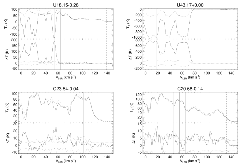
Figure 2: Example H i E/A analysis for four H ii regions. The top panel of each plot shows the on– (solid line) and off– (dotted line) source average H i spectra. The bottom panel of each plot shows the difference between the off– and on–source spectra (solid line) and our error estimates (dotted lines). The three solid vertical lines mark the RRL velocity and $\pm$10 $\,{\rm km\,s}^{-1}$ of the RRL velocity, and the dashed vertical line marks the tangent point velocity. Sources at the far distance will show absorption between the RRL velocity and the tangent point velocity. Sources at the near distance will show absorption only up to the RRL velocity. Top row: example near (left) and far (right) sources which we assign with high confidence (confidence parameter = A). Bottom row: example near (left) and far (right) sources which we assign with low confidence (confidence parameter = B).

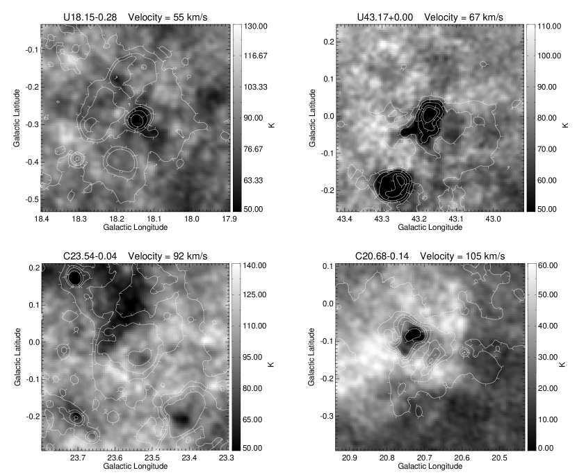
Figure 3: Single channel VGPS images for the Figure 2 H ii regions showing the H i intensity at the highest velocity with detected absorption. The contours are of 21cm VGPS continuum. Tick marks on the contours point towards decreasing values of 21cm continuum intensity. Top row: example near (left) and far (right) sources which we assign with high confidence (confidence parameter = A). Bottom row: example near (left) and far (right) sources which we assign with low confidence (confidence parameter = B).

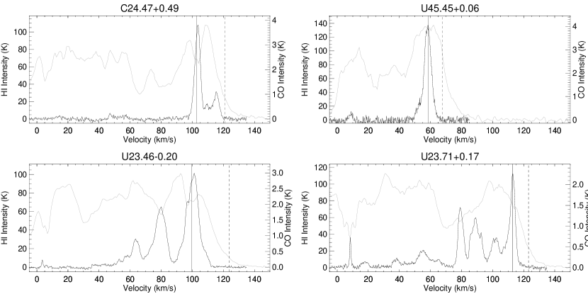
Figure 4: Example H i SA analysis for four H ii regions. The spectrum shown in gray is H i while the spectrum shown in black is ${}^{13}{\rm CO}$. The solid vertical line marks the velocity of the ${}^{13}{\rm CO}$ associated with the H ii region found in Paper I, and the dashed vertical line marks the tangent point velocity. Sources at the near distance show H i absorption at the velocity of ${}^{13}{\rm CO}$ emission. Sources at the far distances show no H i absorption at the velocity of ${}^{13}{\rm CO}$ emission. Top row: example near (left) and far (right) sources which we assign with high confidence (confidence parameter = A). Bottom row: example near (left) and far (right) sources which we assign with low confidence (confidence parameter = B).

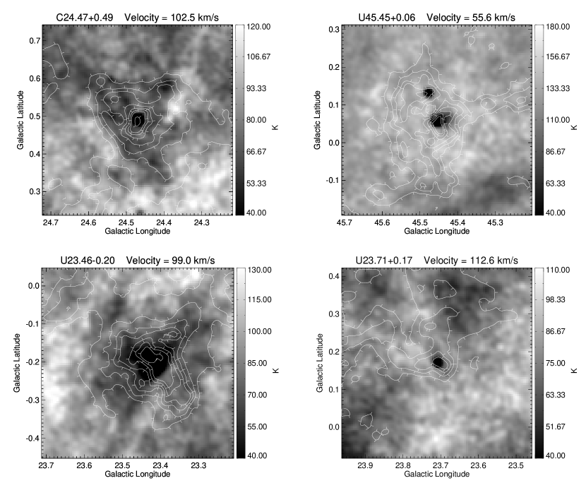
Figure 5: Single channel VGPS images for the Figure 4 H ii regions at the velocity of peak ${}^{13}{\rm CO}$ intensity used in the H i SA analysis. The contours are of integrated ${}^{13}{\rm CO}$ intensity, $W_{\rm 13CO}$. Tick marks on the contours point towards decreasing values of $W_{\rm 13CO}$. Top row: example near (left) and far (right) sources which we assign with high confidence (confidence parameter = A). Bottom row: example near (left) and far (right) sources which we assign with low confidence (confidence parameter = B). The two top images and bottom right image show strong absorption from the H ii region radio continuum at image center; these positions with strong radio continuum emission were not used in the H i SA analysis.

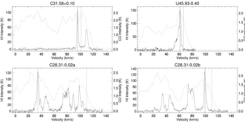
Figure 6: Example H i SA analysis for four H ii regions whose KDA cannot be resolved using the H i E/A method. The plot formats are those of Figure 4. In the top row, the source velocities are very near the tangent point velocities, and yet the H i SA analysis is able to resolve the KDA; the top left source is at the near distance while the top right source is at the far distance. In the bottom row, two H ii regions are located along the same line of sight, but the H i SA analysis is able to resolve the KDA for both sources.; C28.31$-$0.02a is at the far distance while C28.31$-$0.02b is at the near distance.

Figure 7: The ratio of far to near sources plotted as a function of the average H ii region integrated intensity, $W_{\rm 13CO}$. The solid line shows this relationship for a sample of H ii region/${}^{13}{\rm CO}$ cloud complexes defined by 75% of the peak ${}^{13}{\rm CO}$ value. The dashed line shows the relationship defined by 85% of the peak ${}^{13}{\rm CO}$ value.

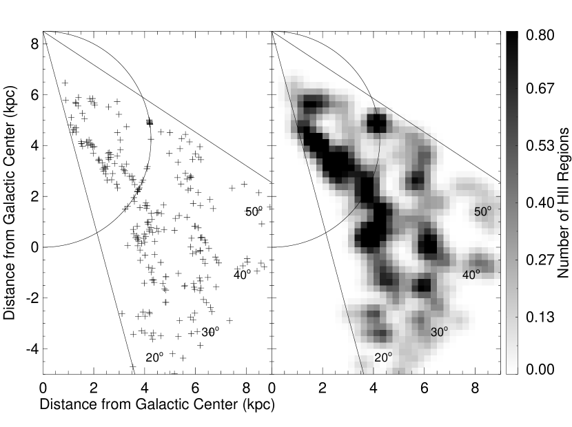
Figure 8: Galactic Distribution of H ii regions. The straight lines show the longitude range of our sample, $15\arcdeg-56\arcdeg$. The half-circle indicates the tangent point distance, and is the locus of subcentral points. The left panel plots shows the positions for all regions with KDA resolved distances. In the right panel, these positions are binned into $0.25\times 0.25$ $\,{\rm kpc}$ pixels, and the resultant image smoothed with a $5\times 5$ pixel Gaussian filter.

Figure 9: Distribution of Galactocentric radii for our H ii region sample. The distribution is shown using 0.25 kpc bins. The peaks at 4.5 and 6 kpc in this distribution correspond to the radii of the circular arc features seen in Figure 8.

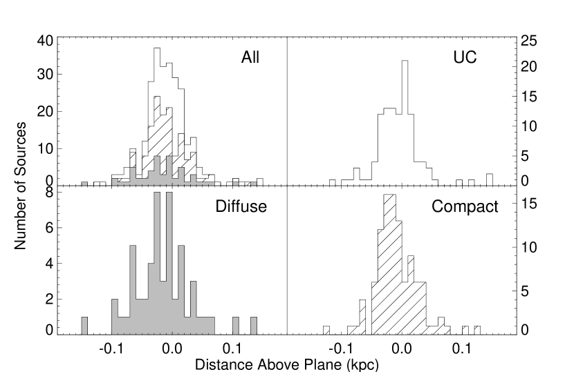
Figure 10: Distribution of height above the plane for the sources with resolved distance ambiguities. Ultra compact sources are shown open, compact sources are shown hatched, and diffuse sources are shown in gray. The top left panel is the stacked histogram of all three categories of H ii regions such that the outer line shows the entire distribution. The other three panels show the distribution for the three categories of H ii regions.

References

- Anderson et al. (2008) Anderson, L. D., Bania, T. M., Jackson, J. M., Clemens, D. P., Heyer, M., Simon, R., Shah, R. Y., Rathborne, J. M. 2008, submitted (Paper I)
- Araya et al. (2002) Araya, E., Hofner, P., Churchwell, E., & Kurtz, S. 2002, ApJS, 138, 63
- Bania & Lockman (1984) Bania, T. M. & Lockman, F. J., 1984, ApJ, 54, 513
- Benjamin et al. (2005) Benjamin, R. A., et al. 2005, ApJ, 630, 149
- Brand (1986) Brand, J. 1986, PhD Thesis, Leiden Univ. (Netherlands)
- Bronfman et al. (2000) Bronfman L., Casassus S., May J., Nyman L. A. 2000, A&A, 358, 521
- Burton (1971) Burton, W. B. 1971, A&A, 10, 76
- Burton & Gordon (1978) Burton, W. B. & Gordon, M. A. 1978, ApJ, 63, 7
- Burton, Liszt, & Baker (1978) Burton, W. B., Liszt, H. S., & Baker, P. L. 1978, ApJ, 219, 67
- Busfield et al. (2006) Busfield, A. L., Purcell, C. R., Hoare, M. G., Lumsden, S. L., Moore, T. J. T., Oudmaijer, R. D. 2006, MNRAS, 366, 1096
- Churchwell, Walmsley, & Cesaroni (1990) Churchwell, E., Walmsley, C. M., & Cesaroni, R. 1990, A&AS, 83, 119
- Clemens (1985) Clemens, D. P. 1985, ApJ, 295, 422
- Conti & Crowther (2004) Conti, P. S. & Crowther, P. A. 2004, MNRAS, 355, 899
- Downes et al. (1980) Downes, D., Wilson, T. L., Bieging, J., & Wink, J. 1980, A&AS, 40, 379
- Fich, Blitz & Stark (1989) Fich, M., Blitz, L. & Stark, A. A. 1989, ApJ, 342, 272
- Fish et al. (2003) Fish, V. L., Reid, M. J., Wilner, D. J., & Churchwell, E. 2003, ApJ, 587, 701
- Flynn et al. (2004) Flynn, E. S., Jackson, J. M., Simon, R., Shah, R. Y., Bania, T. M. & Wolfire, M. 2004, ASP Conference Series, 317, 44
- Gibson et al. (2000) Gibson, S. J., Taylor, A. R., Higgs, L. A., & Dewdney, P. E. 2000, ApJ, 540, 851
- Gibson et al. (2005) Gibson S. J., Taylor, A. R., Higgs, L. A, Brunt, C. M., & Dewdney, P.E. 2005, ApJ, 626, 195
- Giveon et al. (2005) Giveon, U., Becker, R. H., Helfand, D. J., & White, R. L. 2005, AJ, 130, 156
- Goldsmith & Li (2005) Goldsmith, P. F. & Li, D. 2005, 622, 938
- Jackson et al. (2002) Jackson, J. M., Bania, T. M., Simon, R., Kolpak, M., Clemens, D. P. & Heyer, M. 2002, ApJ, 566, 81
- Jackson et al. (2006) Jackson, J. M., Rathborne, J. M., Shah, R. Y., Simon, R., Bania, T. M., Clemens, D. P., Chambers, E. T., Johnson, A. M., Dormody, M. & Lavoie, R. 2006, ApJS, 163, 145
- Li & Goldsmith (2003) Li, D., & Goldsmith, P. F. 2003, ApJ, 585, 823
- Knapp (1974) Knapp, G. R. 1974, AJ, 79, 527
- Kolpak et al. (2003) Kolpak, M. A., Jackson, J. M., Bania, T. M., & Clemens, D. P. 2003, ApJ, 582, 756
- Kuchar & Bania (1993) Kuchar, T. A & Bania, T. M. 1993, ApJ, 414, 664
- Kuchar & Bania (1994) Kuchar, T. A. & Bania, T. M. 1994, ApJ, 436, 117
- Levinson & Brown (1980) Levinson, F. H. & Brown, R. L. 1980, ApJ, 242, 416
- Lockman (1989) Lockman, F. J. 1989, ApJS, 71, 469
- Lockman, Pisano, & Howard (1996) Lockman, F. J, Pisano, D. J., & Howard, G. J., ApJ, 472, 173
- Liszt, Burton & Bania (1981) Liszt, H. S., Burton, W. B., & Bania, T. M. 1981, ApJ, 246, 74
- McClure-Griffiths et al. (2005) McClure-Griffiths, N.M., Dickey, J.M., Gaensler, B.M., Green, A.J., Haverkorn, M., Strasser, S. 2005, ApJS, 158, 178
- McClure-Griffiths & Dickey (2007) McClure-Griffiths, N. M. & Dickey, J. 2007, ApJ, 671, 427
- Paladini, Davies, & Dezotti (2004) Paladini, R., Davies, R. D., & DeZotti, G. 2004, 347, 237
- Payne, Salpeter & Terzian (1980) Payne, H. E., Salpeter, E. E. & Terzian, Y. 1980, ApJ, 240, 499
- Peters & Bash (1983) Peters, W. L. & Bash, F. N. 1983, Proc. Astr. Soc. Australia, 5, 224
- Peters & Bash (1987) Peters, W. L. & Bash, F. N. 1987, ApJ, 317, 646
- Reed (2006) Reed, B. C. 2006, J. R. Astron. Soc. Canada, 100, 146
- Russeil & Castets (2004) Russeil, D. & Castets, A. 2004, A&A, 417, 107
- Simon et al. (2001) Simon, R., Jackson, J. M., Clemens, D. P., & Bania, T. M. 2001, ApJ, 551, 747
- Sewilo, et al. (2004) Sewilo, M., Churchwell, E., Kurtz, S., Goss, W. M., Hofner, P. 2004, ApJ, 605, 285
- Stark & Brand (1989) Stark, A. A. & Brand, J. 1989, ApJ, 339, 763
- Stil et al. (2006) Stil, J. M., et al. 2006, AJ, 132, 1158
- Wannier et al. (1991) Wannier, P. G., Lichten, S. M., Andersson, B. G., & Morris, M. 1991, ApJS, 75, 987
- Watson et al. (2003) Watson, C., Araya, E., Sewilo, M., Churchwell, E., Hofner, P., & Kurtz, S. 2003, ApJ, 587, 714
- Williams & Maddalena (1996) Williams, J. P. & Maddelena, R. J. 1996, ApJ, 464, 247
- Wilson (1972) Wilson, T. L. 1972, A&A, 19, 354
- Wink, Altenhoff & Mezger (1982) Wink, J. E., Altenhoff, W. J., & Mezger, P. G. 1982, A&A, 108, 227