A branch-and-bound feature selection algorithm for U-shaped cost functions

Abstract

This paper presents the formulation of a combinatorial optimization problem with the following characteristics: $i$.the search space is the power set of a finite set structured as a Boolean lattice; $ii$.the cost function forms a U-shaped curve when applied to any lattice chain. This formulation applies for feature selection in the context of pattern recognition. The known approaches for this problem are branch-and-bound algorithms and heuristics, that explore partially the search space. Branch-and-bound algorithms are equivalent to the full search, while heuristics are not. This paper presents a branch-and-bound algorithm that differs from the others known by exploring the lattice structure and the U-shaped chain curves of the search space. The main contribution of this paper is the architecture of this algorithm that is based on the representation and exploration of the search space by new lattice properties proven here. Several experiments, with well known public data, indicate the superiority of the proposed method to SFFS, which is a popular heuristic that gives good results in very short computational time. In all experiments, the proposed method got better or equal results in similar or even smaller computational time.

I Introduction

A combinatorial optimization algorithm chooses the object of minimum cost over a finite collection of objects, called search space, according to a given cost function. The simplest architecture for this algorithm, called full search, access each object of the search space, but it does not work for huge spaces. In this case, what is possible is to access some objects and choose the one of minimum cost, based on the observed measures. Heuristics and branch-and-bound are two families of algorithms of this kind. An heuristic algorithm does not have formal guaranty of finding the minimum cost object, while a branch-and-bound algorithm has mathematical properties that guarantee to find it.

Here, it is studied a combinatorial optimization problem such that the search space is composed of all subsets of a finite set with $n$ points (i.e., a search space with $2^{n}$ objects), organized as a Boolean lattice, and the cost function has a U-shape in any chain of the search space or, equivalently, the cost function has a U-shape in any maximal chain of the search space.

This structure is found in some applied problems such as feature selection in pattern recognition [dudahart2000chap1, jaduma:2000] and W-operator window design in mathematical morphology [dmartins2006]. In these problems, a minimum subset of features, that is sufficient to represent the objects, should be chosen from a set of $n$ features. In W-operator design, the features are points of a finite rectangle of $Z^{2}$ called window. The U-shaped functions are formed by error estimation of the classifiers or of the operators designed or by some measures, as the entropy, on the corresponding estimated join distribution. This is a well known phenomenon in pattern recognition: for a fixed amount of training data, the increasing number of features considered in the classifier design induces the reduction of the classifier error by increasing the separation between classes until the available data becomes too small to cover the classifier domain and the consequent increase of the estimation error induces the increase of the classifier error. Some known approaches for this problem are heuristics. A relatively well succeeded heuristic algorithm is SFFS [pudil94], which gives good results in relatively small computational time.

There is a myriad of branch-and-bound algorithms in the literature that are based on monotonicity of the cost-function [frank, nakariyakul, wang, yang]. For a detailed review of branch-and-bound algorithms, refer to [somol]. If the real distribution of the joint probability between the patterns and their classes were known, larger dimensionality would imply in smaller classification errors. However, in practice, these distributions are unknown and should be estimated. A problem with the adoption of monotonic cost-functions is that they do not take into account the estimation errors committed when many features are considered (“curse of dimensionality” also known as “U-curve problem” or “peaking phenomena” [jaduma:2000]).

This paper presents a branch-and-bound algorithm that differs from the others known by exploring the lattice structure and the U-shaped chain curves of the search space.

Some experiments were performed to compare the SFFS to the U-curve approach. Results obtained from applications such as W-operator window design, genetic network architecture identification and eight UCI repository data sets show encouraging results, since the U-curve algorithm beats (i.e., finds a node with smaller cost than the one found by SFFS) the SFFS results in smaller computational time for 27 out of 38 data sets tested. For all data sets, the U-curve algorithm gives a result equal or better than SFFS, since the first covers the complete search space.

Though the results obtained with the application of the method developed to pattern recognition problems are exciting, the great contribution of this paper is the discovery of some lattice algebra properties that lead to a new data structure for the search space representation, that is particularly adequate for updates after up-down lattice interval cuts (i.e., cuts by couples of intervals [0,X] and [X,W]). Classical tree based search space representations does not have this property. For example, if the Depth First Search were adopted to represent the Boolean lattice only cuts in one direction could be performed.

Following this introduction, Section 2 presents the formalization of the problem studied. Section 3 describes structurally the branch-and-bound algorithm designed. Section 4 presents the mathematical properties that support the algorithm steps. Section 5 presents some experimental results comparing U-curve to SFFS. Finally, Conclusion discusses the contributions of this paper and proposes some next steps of this research.

II The Boolean U-curve optimization problem

Let $W$ be a finite subset, $\mathscr{P}(W)$ be the collection of all subsets of $W$, $\subseteq$ be the usual inclusion relation on sets and, $|W|$ denote the cardinality of $W$. The search space is composed by $2^{|W|}$ objects organized in a Boolean lattice.

The partially ordered set $(\mathscr{P}(W),\subseteq)$ is a complete Boolean lattice of degree $|W|$ such that: the smallest and largest elements are, respectively, $\emptyset$ and $W$; the sum and product are, respectively, the usual union and intersection on sets and the complement of a set $X$ in $\mathscr{P}(W)$ is its complement in relation to $W$, denoted by $X^{c}$.

Subsets of $W$ will be represented by strings of zeros and ones, with $0$ meaning that the point does not belong to the subset and $1$ meaning that it does. For example, if $W=\{(-1,0),(0,0),$ $(+1,0)\}$, the subset $\{(-1,0),(0,0)\}$ will be represented by $110$. In an abuse of language, $X=110$ means that $X$ is the set represented by $110$.

A chain $\mathcal{A}$ is a collection $\{A_{1},A_{2},\ldots,A_{k}\}\subseteq\mathcal{X}\subseteq\mathscr{P}(W)$ such that $A_{1}\subseteq A_{2}\subseteq\ldots\subseteq A_{k}$. A chain $\mathcal{M}\subseteq\mathcal{X}$ is maximal in $\mathcal{X}$ if there is no other chain $\mathcal{C}\subseteq\mathcal{X}$ such that $\mathcal{C}$ contains properly $\mathcal{M}$.

Let $c$ be a cost function defined from $\mathscr{P}(W)$ to $\mathbb{R}$. We say that $c$ is decomposable in U-shaped curves if, for every maximal chain $\mathcal{M}\subseteq\mathscr{P}(W)$, the restriction of $c$ to $\mathcal{M}$ is a U-shaped curve, i. e., for every $A,X,B\in\mathcal{M}$, $A\subseteq X\subseteq B\Rightarrow\max(c(A),c(B))\geq c(X)$.

Figure 1 shows a complete Boolean lattice $\mathcal{L}$ of degree $4$ with a cost function $c$ decomposable in U-shaped curves. In this figure, it is emphasized a maximal chain in $\mathcal{L}$ and its cost function. Figure 2 presents the curve of the same cost function restricted to some maximal chains in $\mathcal{L}$ and in $\mathcal{X}\subseteq\mathcal{L}$. Note the U-shape of the curves in Figure 2.

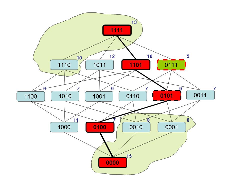
Figure 1: A complete Boolean lattice $\mathcal{L}$ of degree $4$ and the cost function decomposable in U-shaped curves. $\mathcal{X}=\mathcal{L}-\{0000,0010,0001,1110,1111\}$ is a poset obtained from $\mathcal{L}$. A maximal chain in $\mathcal{L}$ is emphasized. The element $0111$ is the global minimum element and $0101$ is the local minimum element in the maximal chain.

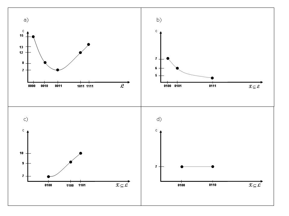
Figure 2: The four possible representaion of the cost function $c$ restricted to some maximal chains in $\mathcal{L}$ (a) and in $\mathcal{X}\subseteq\mathcal{L}$ (b-d) of Figure 1.

Our problem is to find the element (or elements) of minimum cost in a Boolean lattice of degree $|W|$. The full search in this space is an exponential problem, since this space is composed by $2^{|W|}$ elements. Thus, for moderately large $|W|$, the full search becomes unfeasible.

III The U-curve algorithm

The U-shaped format of the restriction of the cost function to any maximal chain is the key to develop a branch-and-bound algorithm, the U-curve algorithm, to deal with the hard combinatorial problem of finding subsets of minimum cost.

Let $A$ and $B$ be elements of the Boolean lattice $\mathcal{L}$. An interval $[A,B]$ of $\mathcal{L}$ is the subset of $\mathcal{L}$ given by $[A,B]=\{X\in\mathcal{L}:A\subseteq X\subseteq B\}$. The elements $A$ and $B$ are called, respectively, the left and right extremities of $[A,B]$. Intervals are very important for characterizing decompositions in Boolean lattices [Banon, Salas].

Let $R$ be an element of $\mathcal{L}$. In this paper, intervals of the type $[\emptyset,R]$ and $[R,W]$ are called, respectively, lower and upper intervals. The right extremity of a lower interval and the left extremity of an upper interval are called, respectively, lower and upper restrictions. Let $\mathcal{R}_{L}$ and $\mathcal{R}_{U}$ denote, respectively, collections of lower and upper intervals. The search space will be the poset $\mathcal{X}(\mathcal{R}_{L},\mathcal{R}_{U})$ obtained by eliminating the collections of lower and upper restrictions from $\mathcal{L}$, i. e., $\mathcal{X}(\mathcal{R}_{L},\mathcal{R}_{U})=\mathcal{L}-\bigcup\{[\emptyset,R]:R\in\mathcal{R}_{L}\}-\bigcup\{[R,W]:R\in\mathcal{R}_{U}\}$. In cases in which only the lower or the upper intervals are eliminated, the resulting search space is denoted, respectively, by $\mathcal{X}(\mathcal{R}_{L})$ and $\mathcal{X}(\mathcal{R}_{U})$ and given, respectively, by $\mathcal{X}(\mathcal{R}_{L})=\mathcal{L}-\bigcup\{[\emptyset,R]:R\in\mathcal{R}_{L}\}$ and $\mathcal{X}(\mathcal{R}_{U})=\mathcal{L}-\bigcup\{[R,W]:R\in\mathcal{R}_{U}\}$.

The search space is explored by an iterative algorithm that, at each iteration, explores a small subset of $\mathcal{X}(\mathcal{R}_{L},\mathcal{R}_{U})$, computes a local minimum, updates the list of minimum elements found and extends both restriction sets, eliminating the region just explored. The algorithm is initiated with three empty lists: minimum elements, lower and upper restrictions. It is executed until the whole space is explored, i. e., until $\mathcal{X}(\mathcal{R}_{L},\mathcal{R}_{U})$ becomes empty. The subset of $\mathcal{X}(\mathcal{R}_{L},\mathcal{R}_{U})$ eliminated at each iteration is defined from the exploration of a chain, which may be done in down-up or up-down direction. Algorithm 1 describes this process. The direction selection procedure (line 5) can use a random or an adaptative method. The random method states a static probability to select the down-up or up-down direction. The adaptative method calculates a new probability to each direction giving more probability to down-up direction if most of the local minima is closest to the bottom of the lattice and up-down otherwise.

Algorithm 1 U-curve-algorithm()

1:  $\mathcal{M}$ $\Leftarrow\emptyset$

2:  $\mathcal{R}_{L}\Leftarrow\emptyset$

3:  $\mathcal{R}_{U}\Leftarrow\emptyset$

4:  while $\mathcal{X}(\mathcal{R}_{L},\mathcal{R}_{U})\neq\emptyset$ do

5:     direction $\Leftarrow$ Select-Direction()

6:     if direction is UP then

7:        Down-Up-Direction($\mathcal{R}_{L}$, $\mathcal{R}_{U}$)

8:     else

9:        Up-Down-Direction($\mathcal{R}_{L}$, $\mathcal{R}_{U}$)

10:     end if

11:  end while

An element $C$ of the poset $\mathcal{X}\subseteq\mathcal{L}$ is called a minimal element of $\mathcal{X}$, if there is no other element $C^{\prime}$ of $\mathcal{X}$ with $C^{\prime}\subset C$. In Figure 1, the minimal elements of $\mathcal{X}(\mathcal{R}_{L})$ are: $1000$, $0100$ and $0011$. If the down-up direction is chosen, the Down-Up-Direction procedure is performed (algorithm 2):

• Minimal-Element procedure calculates a minimal element $B$ of the poset $\mathcal{X}(\mathcal{R}_{L})$. Only the lower restriction set is used to calculate the minimal element $B$. An element $B$ is said to be covered by the lower restriction set $\mathcal{R}_{L}$, if $\exists R\in\mathcal{R}_{L}:B\subseteq R$, and $B$ is said to be covered by the upper restriction set $\mathcal{R}_{U}$, if $\exists R\in\mathcal{R}_{U}:R\subseteq B$. When the calculated $B$ is covered by an upper restriction, it is discarded, i.e., the lower restriction set is updated with $B$ and a new iteration begins (lines 1-5).

• The down-up direction chain exploration procedure begins with a minimal element $B$ and flows by random selection of upper adjacent elements from the current poset $\mathcal{X}(\mathcal{R}_{L},$ $\mathcal{R}_{U})$ until it finds the U-curve condition, i. e., the last element selected ($B$) has cost bigger than the previous one ($M$) (lines 7-11).

• At this point, the element $M$ is the minimum element of the chain explored, $A$ and $B$ are, respectively, the lower and upper adjacent elements of $M$ (i.e., $A\subset M\subset B$ and $\{X\in\mathscr{P}(W):A\subset M\}=\{X\in\mathscr{P}(W):M\subset B=\emptyset$) by construction, $c(A)\leq c(M)\leq C(B)$. It can be proved that any element $C$ of $\mathcal{X}(\mathcal{R}_{L},\mathcal{R}_{U})$, with $C\subset A$, has cost bigger than $A$ and, any element $D$ of $\mathcal{X}(\mathcal{R}_{L},\mathcal{R}_{U})$, with $B\subset D$, has cost bigger than $B$. By using this property, the lower and upper restrictions can be updated, respectively, by $A$ and $B$ (lines 12-17). Figure 3 shows a schematic representation of the first iteration of the algorithm and the elements contained in the intervals $[\emptyset,A=1\ldots 1010\ldots 0]$ and $[B=1\ldots 11110\ldots 0,W]$.

• The result list can be updated with $M$ (line 18) , i. e., $M$ will be included in the result list if it has cost lower than the elements already saved in the list. The result list can save a pre-defined number of elements with low costs or only elements with the overall minimum cost.

• In order to prevent visiting the element $M$ more than once, a recursive procedure called minimum exhausting procedure is performed (line 19)

Algorithm 2 Down-Up-Direction(ElementSet $\mathcal{R}_{L}$, ElementSet $\mathcal{R}_{U}$)

1:  $B\Leftarrow$ Minimal-Element($\mathcal{R}_{L}$)

2:  if $B$ is covered by $\mathcal{R}_{U}$ then

3:     Update-Lower-Restriction($B$, $\mathcal{R}_{L}$)

4:     return  

5:  end if

6:  $M\Leftarrow$ null

7:  repeat

8:     $A\Leftarrow M$

9:     $M\Leftarrow B$

10:     $B\Leftarrow$ Select-Upper-Adjacent($M$, $\mathcal{R}_{L}$, $\mathcal{R}_{U}$)

11:  until $c(B)>c(M)$ or $B=$ null

12:  if $A\neq$ null then

13:     Update-Lower-Restriction($A$, $\mathcal{R}_{L}$)

14:  end if

15:  if $B\neq$ null then

16:     Update-Upper-Restriction($B$, $\mathcal{R}_{U}$)

17:  end if

18:  Update-Results($M$)

19:  Minimum-Exhausting($M$, $\mathcal{R}_{L}$, $\mathcal{R}_{U}$)

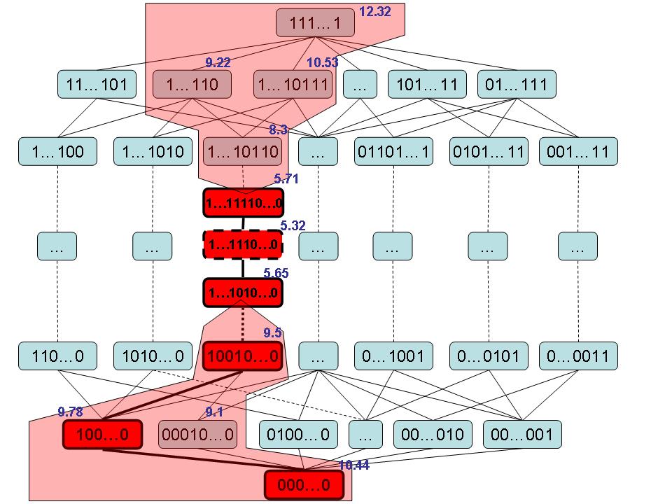
Figure 3: A schematic representation of a step of the algorithm, the detached areas represents the elements contained in a lower and upper restrictions.

An element is called a minimum exhausted element in $\mathcal{L}$ if all its adjacents elements (upper and lower) have cost bigger than it. This definition can be extended to the poset $\mathcal{X}(\mathcal{R}_{L},\mathcal{R}_{U})$, i. e., all its adjacent elements (upper and lower) in $\mathcal{X}(\mathcal{R}_{L},\mathcal{R}_{U})$ have cost bigger than it. In Figure 1 we can see that the elements $1010$, $1001$ and $0111$ are minimum exhauted elements in $\mathcal{X}(\mathcal{R}_{L},\mathcal{R}_{U})$, but $1001$ is not a minimum exhauted element in $\mathcal{L}$. In this paper, the term minimum exhausted will be applied always refering to a poset $\mathcal{X}(\mathcal{R}_{L},\mathcal{R}_{U})$.

Algorithm 3 Minimum-Exhausting(Element $M$, ElementSet $\mathcal{R}_{L}$, ElementSet $\mathcal{R}_{U}$)

1:  Push $M$ to $\mathcal{S}$

2:  while $\mathcal{S}$ is not empty do

3:     $T\Leftarrow$ Top($\mathcal{S}$)

4:     MinimumExhausted $\Leftarrow$ true

5:     for all $A$ adjacent of $T$ in $\mathcal{X}(\mathcal{R}_{L},\mathcal{R}_{U})$ and $A\not\in\mathcal{S}$ do

6:        if c($A$) $\leq$ c($T$) then

7:           Push $A$ to $\mathcal{S}$

8:           MinimumExhausted $\Leftarrow$ false

9:        else

10:           if $A$ is upper adjacent of $T$ then

11:              Update-Upper-Restriction($A$, $\mathcal{R}_{U}$)

12:           else

13:              Update-Lower-Restriction($A$, $\mathcal{R}_{L}$)

14:           end if

15:        end if

16:     end for

17:     if MinimumExhausted then

18:        Pop $T$ from $\mathcal{S}$

19:        Update-Results($T$)

20:        Update-Lower-Restriction($T$, $\mathcal{R}_{L}$)

21:        Update-Upper-Restriction($T$, $\mathcal{R}_{U}$)

22:     end if

23:  end while

24:  return  

The minimum exhausting procedure (Algorithm 3) is a recursive process that visit all the adjacent elements of a given element $M$ and turn all of them into minimum exhausted elements in the resulting poset $\mathcal{X}(\mathcal{R}_{L},\mathcal{R}_{U})$. It uses a stack $\mathcal{S}$ to perform the recursive process. $\mathcal{S}$ is initialized by pushing $M$ to it and the process is performed while $\mathcal{S}$ is not empty (lines 2-22). At each iteration, the algorithm processes the top element $T$ of $\mathcal{S}$: all the adjacent elements (upper and down) of $T$ in $\mathcal{X}(\mathcal{R}_{L},\mathcal{R}_{U})$ and not in $\mathcal{S}$ are checked. If the cost of an adjacent element $A$ is lower (or equal) than the cost of $T$ then $A$ is pushed to $\mathcal{S}$. If the cost of $A$ is bigger than the cost of $T$ then one of the restriction sets can be updated with $A$, lower restriction set if $A$ is lower adjacent of $T$ and upper restriction set if $A$ is upper adjacent of $T$ (lines 5-16). If $T$ is a minimum exhausted element in $\mathcal{X}(\mathcal{R}_{L},\mathcal{R}_{U})$, i. e., there is no adjacent element $A$ in $\mathcal{X}(\mathcal{R}_{L},\mathcal{R}_{U})$ with cost lower than $T$, then $T$ is removed from $\mathcal{S}$ and, also, the restriction sets and the result list are updated with $T$ (lines 19-21). At the end of this procedure all the elements processed are minimum-exhausted elements in $\mathcal{X}(\mathcal{R}_{L},\mathcal{R}_{U})$.

Figure 4 shows a graphical representation of the minimum exhausting process. 4-A shows a chain construction process in up direction, the chain has its edges emphasized. The element $M=010101$ (orange-colored) has the minimum cost over the chain. The elements in black are the elements eliminated from the search space by the restrictions obtained by the lower and upper adjacent elements of the local minimum $M$. The stack begins with the element $M$. Figure 4-B shows the first iteration of the minimum exhausting process. The arrows in red and the elements in red indicates the adjacents elements of $M$ (top of the stack) that have cost lower (or equal) than it. These elements $010001$ and $010111$ are pushed to the stack. The adjacent elements of $M$ with cost bigger than it can update the restriction sets, i. e., the lower adjacent element $000101$ updates the lower restriction set and the upper adjacent element $000101$ updates the upper restriction set. Figure 4-C shows the second iteration: the adjacent elements $010011$ and $000111$ with cost lower (or equal) than the new top element $010111$ are pushed to the stack and the other adjacent elements $010110$ and $011111$ with cost bigger than $010111$ update, respectively, the lower and upper restriction sets. In Figure 4-D the element $000111$ is a minimum exhausted element (grey color) in $\mathcal{X}(\mathcal{R}_{L},\mathcal{R}_{U})$ and it is is removed from stack. In Figure 4-E the elements eliminated by the new interval $[\emptyset,000111]$ and $[000111,W]$ are turned into black color. At this point, $010011$ is a minimum exhausted (grey color) in $\mathcal{X}(\mathcal{R}_{L},\mathcal{R}_{U})$ and it is removed from stack. From Figure 4-F to Figure 4-H all the elements are removed from stack and the elements removed by the new restrictions are turned into black color. Figure 4-H shows all the elements removed from a single minimum exhausted process.

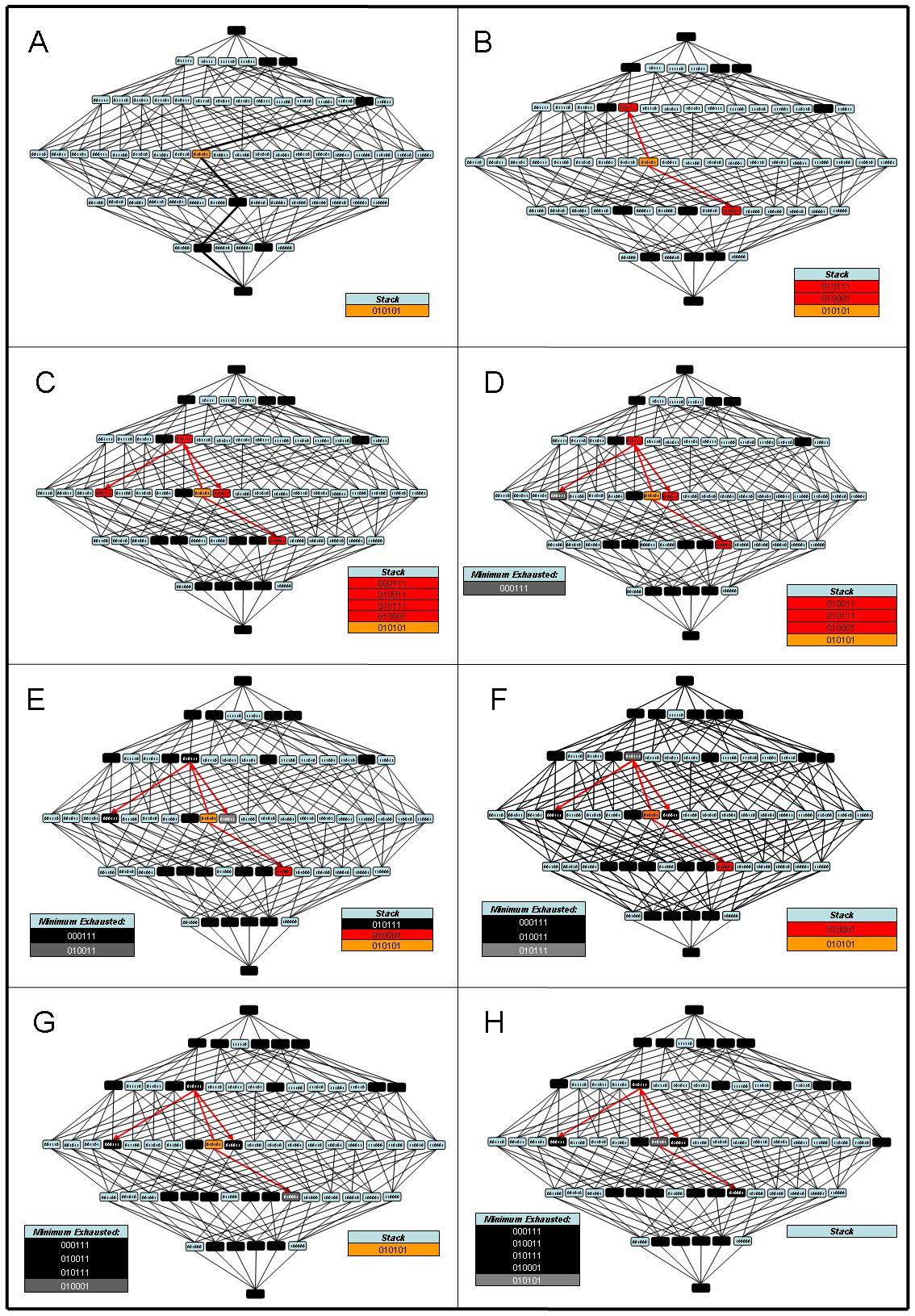
Figure 4: Representation of the minimum exhausting process.

The procedures to calculate minimal and maximal elements and the procedure to update lower and upper restriction sets will be discussed in the next section.

IV Mathematical foundations

This section introduces mathematical foundations of some modules of the algorithm.

IV-A Minimal and Maximal Construction Procedure

Each iteration of the algorithm requires the calculation of a minimal element in $\mathcal{X}(\mathcal{R}_{L})$ or a maximal element in $\mathcal{X}(\mathcal{R}_{U})$. It is presented here a simple solution for that. The next theorem is the key for this solution.

Theorem 1. For every $A\in\mathcal{X}(\mathcal{R}_{L})$,

$A\in\mathcal{X}(\mathcal{R}_{L})\Leftrightarrow A\cap R^{c}\neq\emptyset,\forall R\in\mathcal{R}_{L}$.

Proof:

(in Appendix Section)

Algorithm 4 implements the minimal construction procedure. It builds a minimal element $C$ of the poset $\mathcal{X}(\mathcal{R}_{L})$. The process begins with $C=(\underbrace{1\ldots 1}_{n})$ and $S=(\underbrace{1\ldots 1}_{n})$ and executes a $n$-loop (lines 3-16) trying to remove components from $C$. At each step, a component $k,k\in\{1,\ldots,n\}$ is chosen exclusively from $S$ ($S$ prevents multi-selecting). If the element $C^{\prime}$ resulted from $C$ by removing the component $k$ is contained in $\mathcal{X}(\mathcal{R}_{L})$ then $C$ is updated with $C^{\prime}$ (lines 7-15).

Algorithm 4 Minimal-Element(ElementSet $\mathcal{R}_{L}$)

1:  $C\Leftarrow\underbrace{1\ldots 1}_{n}$

2:  $S\Leftarrow\underbrace{1\ldots 1}_{n}$

3:  while $S\neq\underbrace{0\ldots 0}_{n}$ do

4:     $k\Leftarrow$ random index in $\{1,\ldots,n\}$ where $S[k]=1$

5:     $S[k]\Leftarrow 0$

6:     $C^{\prime}\Leftarrow C\setminus{k}$

7:     RemoveElement $\Leftarrow$ true

8:     for all $R$ in $\mathcal{R}_{L}$ do

9:        if $R^{c}\cap C^{\prime}=\emptyset$ then

10:           RemoveElement $\Leftarrow$ false

11:        end if

12:     end for

13:     if RemoveElement then

14:        $C\Leftarrow C^{\prime}$

15:     end if

16:  end while

17:  return  $C$

The minimal element calculated is equal to $\underbrace{1\ldots 1}_{n}$ when $\mathcal{R}_{L}=\{\underbrace{1\ldots 1}_{n}\}$. At this point, the poset $\mathcal{X}(\mathcal{R}_{L},\mathcal{R}_{U})$ is empty and the algorithm stops in the next iteration.

The next theorem proves the correctness of Algorithm 4 .

Theorem 2. The element $C$ of $\mathcal{X}(\mathcal{R}_{L})$ returned by the minimal construction process (Algorithm 4) is a minimal element in $\mathcal{X}(\mathcal{R}_{L})$.