Anonymizing Graphs

Abstract

Motivated by recently discovered privacy attacks on social networks, we study the problem of anonymizing the underlying graph of interactions in a social network. We call a graph $(k,\ell)$-anonymous if for every node in the graph there exist at least $k$ other nodes that share at least $\ell$ of its neighbors. We consider two combinatorial problems arising from this notion of anonymity in graphs. More specifically, given an input graph we ask for the minimum number of edges to be added so that the graph becomes $(k,\ell)$-anonymous. We define two variants of this minimization problem and study their properties. We show that for certain values of $k$ and $\ell$ the problems are polynomial-time solvable, while for others they become NP-hard. Approximation algorithms for the latter cases are also given.

1 Introduction

The popularity of online communities and social networks in recent years has motivated research on social-network analysis. Though these studies are useful in uncovering the underpinnings of human social behavior, they also raise privacy concerns for the individuals involved.

A social network is usually represented as a graph, where nodes correspond to individuals and edges capture relationships between these individuals. For example, in LinkedIn, an online network of professionals, every link between two users specifies a professional relationship between them. In Facebook and Orkut links correspond to friendships. There are online communities that permit any user to access the information of every node in the graph and view its neighbors. However, many communities are increasingly restricting access to the personal information of other users. For example, in LinkedIn, a user can only see the profiles of his own friends and their connections.

In this paper, we consider a scenario where the owner of a social network would like to release the underlying graph of interactions for social-network analysis purposes, while preserving the privacy of its users. More specifically, the private information to be protected is the mapping of nodes to real-world entities and interconnections amongst them. Therefore, we design an anonymization framework that tries to hide the identity of nodes by creating groups of nodes that look similar by virtue of sharing many of the same neighbors. We call such nodes anonymized. Our goal is to anonymize all nodes of the graph by introducing minimal changes to the overall graph structure. In this way we can guarantee that the anonymized graph is still useful for social-network analysis purposes.

Recently, Backstrom et. al. [4] have shown that the most simple graph-anonymization technique that removes the identity of each node in the graph, replacing it with a random identification number instead, is not adequate for preserving the privacy of nodes. Specifically, they show that in such an anonymized network, there exists an adversary who can identify target individuals and the link structure between them. However, the problem of designing anonymization methods against such adversaries is not addressed in [4].

Following the work of [4], Hay et. al. [7] have very recently given a definition of graph anonymity: a graph is $k$-anonymous if every node shares the same neighborhood structure with at least $k-1$ other nodes. The definition is recursive, and has some nice properties studied in [7]. However, the focus of [7] is mostly on the properties of the definitions rather than on algorithms to achieve the anonymity requirements.

Motivated by  [4] and [7], Zhou and Pei [18] consider the following definition of anonymity in graphs: a graph is $k$-anonymous if for every node there exist at least $k-1$ other nodes that share isomorphic $1$-neighborhoods. They consider the problem of minimum graph-modifications (in terms of edge additions) that would lead to a graph satisfying the anonymity requirement. Although this definition is interesting, the algorithm presented in [18] is not supported by theoretical analysis. Further, if the anonymity definition is extended to consider the neighborhood structure beyond just the immediate $1$-neighborhood of each node, algorithmic techniques quickly become infeasible.

Despite the fact that privacy concerns in releasing social-network data have been pinpointed, there is no agreement on the definition of privacy or anonymity that should be used for such data. In this paper, we try to move this line of research one step forward by proposing a new definition of graph anonymity that is inline to a certain extent with the definitions provided in [7]. Our definition of anonymity is in a sense less strict than the one proposed in [18]. However, we consider it to be natural, intuitive and more amenable to theoretical analysis.

Intuitively our definition aims to protect an individual from an adversary who knows some subset of the individual’s neighbors in the graph. After anonymization, the hope is that the adversary can no longer identify the target individual because several other nodes in the graph will also share this subset of neighbors. Further, during anonymization, the identifying subset of neighbors themselves will become distorted and harder for the adversary to identify.

The Problem: We define a graph to be $(k,\ell)$-anonymous if for every node $u$ in the graph there exist at least $k$ other nodes that share at least $\ell$ of their neighbors with $u$. In order to meet this anonymity requirement one could transform any graph into a complete graph. For a graph consisting of $n$ nodes this would mean that every node would share $n-2$ neighbors with each of the $n-1$ other nodes. Although such an anonymization would preserve privacy, it would make the anonymized graph useless for any study. For this reason we impose the additional requirement that the minimum number of such edge additions should be made. The aim is to preserve the utility of the original graph, while at the same time satisfying the $(k,\ell)$-anonymity constraint.

Given $k$ and $\ell$ we formally define two variants of the graph-anonymization problem that ask for the minimum number of edge additions to be made so that the resulting graph is $(k,\ell)$-anonymous. We show that for certain values of $k$ and $\ell$ the problems are polynomial-time solvable, while for others they are NP-hard. We also present simple and intuitive approximation algorithms for these hard instances. To summarize our contributions:

• We propose a new definition of graph anonymity building on previously proposed definitions.

• We provide the first formal algorithmic treatment of the graph-anonymization problem.

Besides graph anonymization, the combinatorial problems we study here may also arise in other domains, e.g., graph reliability. We therefore believe that the problem definitions and algorithms we present are of independent interest.

Roadmap: The rest of the paper is organized as follows. In Section 2 we summarize the related work. Section 3 gives the necessary notation and definitions. Algorithms and hardness results for different instances of the $(k,\ell)$-anonymization problem are given in Sections 4, 5, 6 and 7. We conclude in Section 8.

2 Related Work

As mentioned in the Introduction, there has been some prior work on privacy-preserving releases of social-network graphs. The authors in [4] show that the naive approach of simply masking usernames is not sufficient anonymization. In particular, they show that, if an adversary is given the chance to create as few as $\Theta(\log(n))$ new accounts in the network, prior to its release, then he can efficiently recover the structure of connections between any $\Theta(\log^{2}(n))$ nodes chosen apriori. He can do so by identifying the new accounts that he inserted in to the network. The focus of [4] is on revealing the power of such adversaries and not on devising methods to protect against them.

In [7] the authors experimentally evaluate how much background information about the neighborhood of an individual would be sufficient for an adversary to uniquely identify that individual in a naively anonymized graph. Additionally, a new recursive definition of graph anonymity is given. The definition says that a graph is $k$-anonymous if for every structure query there exist $k$ nodes that satisfy it. The definition is constructed for a certain class of structure queries that query the neighborhood structure of the nodes. Our definition of anonymity is inspired by [7], however it is substantially different. Moreover, the focus of our work is on the combinatorial problems arising from our anonymity definition.

Very recently, the authors of [18] consider yet another definition of graph anonymity; a graph is $k$-anonymous if for every node there exist at least $k-1$ other nodes that share isomorphic $1$-neighborhoods. This definition of anonymity in graphs is different from ours. In a sense it is a more strict one. Moreover, though the algorithm presented in [18] seems to work well in practice, no theoretical analysis of its performance is presented. Finally, extending the privacy definition to more than just the $1$-neighborhood of nodes causes the algorithms of [18] to quickly become infeasible.

The problem of protecting sensitive links between individuals in an anonymized social network is considered in [17]. Simple edge-deletion and node-merging algorithms are proposed to reduce the risk of sensitive link disclosure. This work is different from ours in that we are primarily interested in protecting the identity of the individuals while in [17] the emphasis is on protecting the types of links associated with individuals. Also, the combinatorial problems that we need to solve in our framework are very different from the set of problems discussed in [17].

In [6] the authors study the problem of assembling pieces of a graph owned by different parties privately. They propose a set of cryptographic protocols that allow a group of authorities to jointly reconstruct a graph without revealing the identity of the nodes. The graph thus constructed is isomorphic to a perturbed version of the original graph. The perturbation consists of addition and or deletion of nodes and or edges. Unlike that work, we try to anonymize a single graph by modifying it as little as possible. Moreover, our methods are purely combinatorial and no cryptographic protocols are involved.

Korolova et. al. [8] investigate an attack where an adversary strategically subverts user accounts. He then uses the online interface provided by the social network to gain access to local neighborhoods and to piece them together to form a global picture. The authors provide recommendations on what the lookahead of a social network should be to render such attacks infeasible. This work does not consider an anonymized release of the entire network graph and is thus different from ours.

Besides graphs, there has been considerable prior work on anonymizing traditional relational data sets. The line of work on $k$-anonymity found in [1, 11, 9, 12, 14, 10] aims to minimally suppress or generalize public attributes of individuals in a database in such a way that every individual (identifiable by his public attributes) is hidden in a group of size at least $k$. Our notion of graph anonymity draws inspiration from this.

Apart from suppression or generalization techniques, perturbation techniques have also been used to anonymize relational data sets in [2, 3, 5]. Perturbation-based approaches for graph anonymization are also considered in [7, 16]; in that case edges are randomly inserted or deleted to anonymize the graph. We do not consider perturbation-based approaches in this paper.

3 Preliminaries

In this section we formalize our definition of graph anonymity and introduce two natural optimization problems that arise from it.

Throughout the paper we assume that the social-network graph is simple, i.e., it is undirected, unweighted, and contains no self-loops or multi-edges. This is an important category of graphs to study; most of the aforementioned social networks (Facebook, LinkedIn, Orkut) allow only bidirectional links and are thus instances of such simple graphs. We assume that the actual identifiers of individual nodes are removed prior to further anonymization. Our definition for graph anonymity is inspired by the notion of $k$-anonymity for relational data wherein each person, identifiable by his public attributes, is required to be hidden in a group of size $k$. In the case of a social-network graph, the publicly-known attributes of a user would be (a subset of) his connections (and interconnections amongst them) within the graph.

Consider a simple unlabelled graph and an adversary who knows that a target individual and some number of his friends form a clique. In the released graph, the adversary could look for such cliques to narrow down the set of nodes that might correspond to the target individual. The goal of an anonymization scheme is to prevent such an adversary from uniquely identifying the individual and his remaining connections in the anonymized graph.

We achieve this by introducing an anonymity property that requires that for every node in the graph, some subset of its neighbors should be shared by other nodes. In this way, an adversary who knows some subset of the neighbors of a target individual and can even pinpoint them in the graph, will not be able to distinguish the target individual from other nodes in the network that share this subset of neighbors. Further, in the process of anonymization, the identifying subset of neighbors itself becomes distorted and harder for the adversary to pinpoint. More formally we define the $(k,\ell)$-anonymity property as follows.

Definition 1 ($(k,\ell)$-anonymity).

A graph $G=(V,E)$ is $(k,\ell)$-anonymous if for each vertex $v\in V$, there exists a set of vertices $U\subseteq V$ not containing $v$ such that $|U|\geq k$ and for each $u\in U$ the vertices $u$ and $v$ share at least $\ell$ neighbors.

Example 1.

A clique of $n$ nodes is $(n-1,n-2)$-anonymous.

To demonstrate the kinds of attacks we hope to protect against, we give another example.

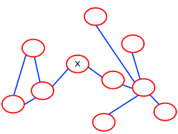
(a) Input graph $G$

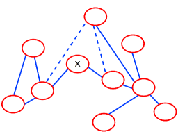
(b) (4,1)-anonymous transformation of $G$

Figure 1: In Figure 1(a) an adversary can identify Alice as the node marked X. Figure 1(b) is a (4,1)-anonymous transformation of the graph.

Example 2.

Consider the graph in Figure 1(a). Suppose an adversary knows that Alice is in this graph and that Alice is connected to a friend who is part of a triangle. There is only one such node in the graph and hence the adversary will be able to determine that the node marked X in the graph uniquely corresponds to Alice. From this he may be able to further infer the identities of Alice’s neighbors and their neighbors as well. Now if the edges shown in dotted lines in Figure 1(b) are added to this graph, the resulting graph is $(4,1)$-anonymous. In this new graph, Alice is no longer the only node connected to a node of a triangle. Further, there is no longer only one triangle in the graph.

Given an input graph $G=(V,E)$ with $n$ nodes, and integers $k$ and $\ell$, our goal is thus to transform the graph into a $(k,\ell)$-anonymous graph. We focus on transformations that allow only additions of edges to the original graph In order for the anonymized graph to remain useful for social-network (or other) studies, we need to ensure that the transformed graph is as close as possible to the original graph. We achieve this by requiring that a minimum number of edges should be added to $G$ so that the $(k,\ell)$-anonymity property holds. This leads us to the following two variants of the $(k,\ell)$-anonymization problem.

Problem 1 (Weak $(k,\ell)$-anonymization).

Given a graph $G=(V,E)$ and integers $k$ and $\ell$, find the minimum number of edges that need to be added to $E$, to obtain a graph $G^{\prime}=(V,E^{\prime})$ that is $(k,\ell)$-anonymous.

The following example illustrates the weak-anonymization problem.

(a) Input graph $G$

(b) Weakly $(k-1,1)$ - anonymized graph $G^{\prime}$

Figure 2: Illustrative example of the difference between weak and strong anonymity.

Example 3.

Consider the input graph $G$ of Figure 2(a). The graph consists of a clique of size $k$ and $2$ nodes $x$ and $y$ connected by an edge. The nodes in the clique are all $(k-1,k-2)$-anonymous. However, the existence of $x$ and $y$ prevents $G$ from being fully $(k-1,1)$-anonymous.

Assume now that we connect both $x$ and $y$ to a single node $u$ of the clique. In this way, we construct graph $G^{\prime}$ shown in Figure 2(b). Obviously, $G^{\prime}$ is $(k-1,1)$-anonymous; all the nodes in $G^{\prime}$ (including $x$ and $y$) have $k-1$ other nodes that share at least one of their neighbors. For $x$ and $y$, this neighbor is node $u$.

The problem in the above example is that graph $G^{\prime}$ satisfies the $(k-1,1)$-anonymity requirement, however, the anonymity of nodes $x$ and $y$ is achieved via node $u$ that was not a part of their initial set of neighbors in $G$. Thus, the goal of having many other nodes sharing the original neighborhood structure of $x$ or $y$ is not necessarily achieved unless we place additional requirements on the anonymization procedure. To this end we introduce the problem of strong anonymization. Strong anonymity places additional restrictions on how anonymity can be achieved and provides better privacy.

Definition 2 (Strong $(k,\ell)$-transformation).

Consider graphs $G=(V,E)$ and $G^{\prime}=(V,E^{\prime})$, so that $E\subseteq E^{\prime}$ and $G^{\prime}$ is $(k,\ell)$-anonymous. For fixed $k$ and $\ell$, we say that $G^{\prime}$ is a strongly-anonymized transformation of $G$, if for every vertex $v\in V$, there exists a set of vertices $U\subseteq V$ not containing $v$ such that $|U|\geq k$ and for each $u\in U$, $|N_{G}(v)\cap N_{G^{\prime}}(u)|\geq$ $\ell$. Here $N_{G}(v)$ is the set of neighbors of $v$ in $G$, and $N_{G^{\prime}}(u)$ is the set of neighbors of $u$ in $G^{\prime}$.

Therefore, if a graph $G^{\prime}$ is a strong $(k,\ell)$-transformation of graph $G$, then each vertex in $G^{\prime}$ is required to have $k$ other vertices sharing at least $\ell$ of its original neighbors in $G$. For this to be possible, every vertex must have at least $\ell$ neighbors in the original graph $G$ to begin with.

Example 4.

Consider again the graph $G$ of Figure 2(a) and its transformation to graph $G^{\prime}$ shown in Figure 2(b). In Example 3 we showed that graph $G^{\prime}$ is $(k-1,1)$-anonymous in the weak sense. However, in order to get a strong $(k-1,1)$-transformation of $G$, we would have to connect each of the nodes $x$ and $y$ to $k-1$ other nodes from the clique.

The definition of a strong $(k,\ell)$-transformation gives rise to the following strong $(k,\ell)$-anonymization problem.

Problem 2 (Strong $(k,\ell)$-anonymization).

Given a graph $G=(V,E)$ and integers $k$ and $\ell$, find the minimum number of edges that need to be added to $E$, to obtain graph $G^{\prime}=(V,E^{\prime})$ that is a strong $(k,\ell)$-transformation of $G$.

Obviously achieving strong anonymity would require the addition of a larger number of edges than weak anonymity. This statement is formalized as follows.

Proposition 1.

Consider input graph $G=(V,E)$ and integers $k$ and $\ell$. Let $G^{\prime}=(V,E^{\prime})$ be the $(k,\ell)$-anonymous graph that is the optimal solution for Problem 1, and $G^{\prime\prime}=(V,E^{\prime\prime})$ be the $(k,\ell)$-anonymous graph that is the optimal solution for Problem 2. Then it holds that $|E^{\prime\prime}|\geq|E^{\prime}|$.

The notion of $(k,\ell)$-anonymity is strongly related to the immediate neighbors of a node in the graph, and how these are shared with other nodes. Therefore, for every node $u$ it is important to know the nodes that are reachable from $u$ via a path of length exactly $2$. Given its importance, we define the notion of $2$-neighborhood of a node as follows.

Definition 3 ($2$-neighborhood).

Given a graph $G=(V,E)$ and a node $v\in V$ we define the $2$-neighborhood of $v$ to be the set of all nodes in $G$ that are reachable from $v$ via paths of length exactly $2$.

We also define two more terms that will be used in the rest of the paper.

Definition 4 (Residual Anonymity).

Consider a graph $G=(V,E)$ that we would like to make $(k,\ell)$-anonymous. Consider any node $v\in V$ and suppose that $k^{\prime}$ other nodes in the graph share at least $\ell$ of $v$’s neighbors. Then, we define the residual anonymity of $v$ to be $r(v)={\text{m}ax}\{k-k^{\prime},0\}$. The residual anonymity of a graph $G=(V,E)$ is defined to be $r(G)=\sum_{v\in V}r(v)$.

We define the concept of a deficient node for nodes that are not $(k,\ell)$-anonymous.

Definition 5 (Deficient Node).

A node $v$ is deficient if $r(v)>0$.

It is the deficient nodes that we need to take care of in order to anonymize a graph. With these definitions in hand, we are now ready to proceed to the technical results of the paper.

4 $(2,1)$-anonymization

In this section we provide polynomial-time algorithms for the weak and strong $(2,1)$-anonymization problems. First, it is easy to see that there is a simple characterization of $(2,1)$-anonymous graphs. This fact is captured in the following proposition.

Proposition 2.

A graph $G=(V,E)$ is $(2,1)$-anonymous if and only if each vertex $u\in V$ is (a) part of a triangle, (b) adjacent to a vertex of degree at least 3, or (c) is the middle vertex in a path of 5 vertices.

The main idea of the algorithms that we develop for $(2,1)$-anonymization is that they add the minimum number of edges so that every vertex of the resulting graph satisfies one of the conditions of Proposition 2. Both algorithms proceed in two phases: the deficit-assignment and the deficit-matching phase. The deficit assignment requires a linear scan of the graph in which deficits are assigned to vertices. Roughly speaking, a deficit of $1$ signifies that the vertex needs to be connected to another vertex of non-zero deficit by the addition of an extra edge. This added edge ensures that the $(2,1)$-anonymity requirement for the vertex or its neighbors will be satisfied. Once the deficits are assigned to vertices the algorithms proceed to the actual addition of edges. The edges are added by taking into account the deficits of all vertices. For example, two vertices both of deficit $1$ can be connected by the addition of a single edge (if they are not already neighbors and are not isolated). In this way, a single edge accommodates a total deficit of $2$. The minimum number of edges to be added can be found via a matching of the vertices with deficits. The matching consists of edges that are not already in the graph. A perfect matching is the matching that satisfies all the deficits. In the case of weak anonymization, this matching can be found in linear time by randomly pairing up non-adjacent vertices with deficits. For strong anonymization, it needs to be explicitly computed by solving the maximum-matching problem over edges that are not already in the graph.

Another key point in the development of our algorithms is that in order to assign deficits it suffices to explore only vertices that are within a distance $4$ from some leaf vertex or from a vertex of degree $2$. Any other vertex can be shown to satisfy the conditions of Proposition 2. Finally, it only requires a case analysis to show that our algorithms optimally assign deficits to vertices, independently of the order in which they traverse the vertices of the input graph during the first phase. For lack of space we only give a sketch of the algorithms and proofs in this section.

4.1 Linear-time weak $(2,1)$-anonymi-zation

As we have already mentioned our algorithm for the weak $(2,1)$-anonymization problem has two phases (1) deficit assignment and (2) deficit matching

Deficit Assignment: First assume that the input graph has no isolated vertices – we will show how to deal with isolated vertices later. For the deficit-assignment phase, the algorithm starts with an unmarked vertex of degree $1$ or $2$ and explores vertices within a distance $4$ of it. Deficits are assigned as follows:

• For an isolated edge $uv$, we assign deficit $1$ to $u$ and deficit $1$ to $v$; it may be that both edges will be added at $u$.

• For an isolated path $uvw$, we assign deficit $1$ to $v$.

• For an isolated path $uvwx$, we assign deficit $1$ to $v$ and deficit $1$ to $w$.

• For a subgraph consisting of a path $uvw$ with adjacent vertices attached to $w$, we assign deficit $1$ to $v$.

• For a component $uvX_{i}$ with vertex $u$ having degree one with vertex $v$ connected to a set of vertices $X_{i}$ such that each $x\in X_{i}$ has degree $1$ (and no other vertices) assign deficit $1$ to $v$. This component corresponds to an isolated star centered at $v$.

• For a component consisting of a square $uvwx$ (isolated square), we assign deficit $1$ to $u$ and deficit $1$ to $w$; it may be that the two edges will be added at $u$ and $v$, or that $u$ and $w$ will be joined.

• For a subgraph consisting of a square $uvwx$ with edges (one or more) $ux_{i}$ coming out of the square, we assign deficit $1$ to $v$.

• For a subgraph consisting of squares $uv_{1}wx_{1}$, $uv_{2}wx_{2}$, $\ldots$, $uv_{j}wx_{j}$, we assign deficit $1$ to one of the $v_{i}$’s.

• Finally, for a subgraph consisting of a vertex $u$ adjacent to vertices $x_{i}$ of degree $1$ and to a vertex $y$ of degree $2$, assign deficit $1$ to $y$.

All the vertices that are visited in this process are marked (that is the assigned deficits cover all marked vertices) and the deficit-assignment process repeats starting with the next unmarked vertex until no more unmarked vertices of degree $1$ or $2$ remain.

Deficit Matching: If the number of vertices with deficit $1$ is $2m$, and $2m\geq 4$ or $2m=2$ – in some case other than an isolated edge $uv$ – then, we need to find any perfect matching amongst these vertices to find the edges to add. The matching of deficits can be done in linear time since any (random) pairing of non-adjacent vertices with non-zero deficits suffices. In this case we add $m$ extra edges. If the number of vertices with deficit $1$ is $2m+1$, then all but one of these vertices can be matched, and a single edge needs to be added to the remaining vertex, connecting it to some vertex of degree at least $2$. This results in a total of $m+1$ extra edges. There are, however, some special cases that we need to take care of first.

Special Cases: Before finding the perfect matching we match all isolated edges to each other. This is because the isolated edges need to be connected in a special way to take care of the deficits at the two ends. For a pair of isolated edges $uv$ and $u^{\prime}v^{\prime}$, we add the edges $uu^{\prime}$ and $vu^{\prime}$ (we treat the two deficits of $1$ at $u$ and $v$ as being concentrated at $u$). In the end we may be left with a single isolated edge $uv$. In this case, two edges need to be added and we can connect them to any other vertex in the graph forming a triangle. Similarly, in the case where the remainder is an isolated star centered at $v$ with vertices $x_{i}$ of degree one, it is enough to add a single edge to connect vertices $x_{j}$ and $x_{j^{\prime}}$ of the star.

Isolated Vertices: It remains to take care of isolated vertices. For this we consider a set of six isolated vertices $u,v,w,u^{\prime},v^{\prime},w^{\prime}$ and we connect them with edges $uv,uw,uu^{\prime},$ $u^{\prime}v^{\prime},u^{\prime}w^{\prime}$. These five edges can take care of the six isolated vertices. In general, the vertices with deficit $1$ can be attached to isolated vertices first, with two exceptions to be considered next. When we have an isolated edge $xy$, one of the two deficits of 1 can be satisfied by connecting $x$ to an isolated vertex, but the other one can also be satisfied by connecting $x$ to an isolated vertex $u$ if $u$ is also made adjacent to two other isolated vertices $v$ and $w$ to obtain the above mentioned component. Similarly if $x$ is only adjacent to vertices $y_{i}$ of degree $1$, then the deficit $1$ at $x$ can only be matched to an isolated $u$ if $u$ is also made adjacent to two other isolated vertices $v$ and $w$. In the end we will be left with fewer than six isolated vertices which each need one edge. These can be connected to any vertex in the graph of degree at least $2$. The optimality follows because a tree on $5$ vertices is optimal saving.

Theorem 1.

The above algorithm solves optimally the weak $(2,1)$-anonymization problem in linear time.

Proof Sketch: It requires a case analysis (that we omit for lack of space) to show that the deficit-assignment scheme we described above is complete and optimal and that the total deficit assigned is independent of the order in which the vertices of the graph are traversed. Since we find a perfect matching, we satisfy these deficits with as few edges as possible, hence, the optimality of the algorithm.

It is also easy to see that the deficit-assignment takes time linear with respect to the number of edges in the graph: first we only consider vertices of degree one or two as starting points. For every such vertex we only have to explore all vertices within a distance $4$. This is because any other vertex can be seen to satisfy one of the conditions of Proposition 2. After each iteration of the deficit assignment, we mark all the vertices that have been visited in this process as marked (that is the assigned deficits cover all visited vertices). The deficit-assignment process continues starting with the next unmarked vertex of degree $1$ or $2$. The scanning of the algorithm requires only linear time with respect to the number of edges in the graph since every traversed edge connects only marked endpoints and thus no edge needs to be traversed more than once by the algorithm.

The deficit-matching phase is also linear since it only requires to find any (random) matching between non-adjacent deficits.

4.2 Polynomial-time strong $(2,1)$-anonymization

The algorithm for solving the strong $(2,1)$-anonymization problem is very similar to the one presented in the previous section, so we only briefly discuss it here. For brevity we avoid mentioning various special cases that are similar to the weak-anonymization problem. The first key difference is that for strong $(2,1)$-anonymization we need to develop a different deficit-assignment scheme. Although the actual structures we have to consider for assigning the deficits are the same we need to assign different deficits to different vertices so that we satisfy the strong anonymity requirement. This is because an edge added at a vertex with assigned deficit can only help the original neighbors of the vertex, and not the vertex itself. The second difference is that in the deficit-matching phase we need to actually solve a maximum-matching problem; not every random pairing of non-adjacent vertices with assigned deficit is a valid solution.

In strong $(2,1)$-anonymization we first have to assume that there are no isolated vertices in the input graph $G$; otherwise strong $(2,1)$-anonymity is not achievable for these vertices.

Deficit Assignment: For the deficit-assignment step, the algorithm starts with an unmarked vertex in the input graph with degree $1$ or $2$ and assigns deficits as follows:

• For an isolated edge $uv$, assign deficit of $2$ at each end.

• For an isolated path $uvwx$, put deficit $1$ at $v$ and at $w$.

• For an isolated square $uvwx$, put deficit $1$ at $u$ and $v$.

• If such a square has edges already coming out of $v$, put just deficit $1$ at $u$.

• If multiple squares $uv_{i}wx_{i}$ all start from vertex $u$, then assign deficit $1$ to one of the $v_{i}$’s.

• For a path $uvw$, put deficit $1$ at each of the $3$ vertices.

• For a vertex of degree at least $3$ attached to vertices of degree $1$, put two deficits of $1$ at degree $1$ vertices.

• If a path starts $uvwx$, with $x$ of degree at least $2$, put deficit $1$ at $v$ and $1$ at $w$.

• If in addition $w$ has other edges coming out of it, put deficit $1$ just at $v$. Otherwise if in addition only $v$ has other edges coming out of it that join to a vertex of degree $1$, put deficit $1$ just at $w$.

All vertices that are visited in the process are marked, and the algorithm proceeds with the next unmarked vertex until there are no unmarked vertices left.

Deficit Matching: For solving the strong $(2,1)$ - anonymization problem exactly we need to solve a maximum-matching problem between the nodes with deficits. This can be done in polynomial time ([13]). Note, that in the weak $(2,1)$-anonymization problem any random pairing of non-adjacent nodes with deficits was sufficient, allowing for a linear-time matching phase. This was because with the exception of isolated edges and isolated paths of length $4$, there was no case in which two vertices of non-zero deficit could be adjacent. This is not the case in the strong anonymization problem, and here a maximum-matching problem needs to be solved over edges that are not already in the graph.

A linear-time deficit-matching algorithm with a small additive error can also be developed. This is summarized in the following theorem.

Theorem 2.

The strong $(2,1)$-anonymization problem can be approximated in linear time within an additive error of 2, and can be solved exactly in polynomial time.

Proof Sketch: It requires again a case analysis to show that the deficit-assignment scheme is optimal and independent of the order in which we traverse the vertices.

Now, if all deficits add up to $m$, they can easily be paired using a greedy linear-time matching algorithm. However, the last $2$ deficits may be assigned to adjacent vertices. So instead of adding $\lceil m/2\rceil$ edges, we may add $\lceil m/2\rceil+2$, for an additive error of 2. If instead we use a maximum-matching algorithm to match as many deficits as possible and satisfy the unmatched deficits individually, the problem can be solved optimally in polynomial time.

5 From $(6,1)$ to $(7,1)$-anonymity

We show here that given a graph that is already (6,1)-anonymous, it is NP-hard to find the minimal number of edges that need to be added to make it either weakly or strongly (7,1)-anonymous. This result provides insight into the complexity of the anonymization problem, showing that it is hard to achieve anonymity even incrementally. The result follows from a reduction from the 1-in-3 satisfiability problem. An instance of 1-in-3 satisfiability consists of triples of Boolean variables $(x,y,z)$ to be assigned values 0 or 1 in such a way that each triple contains one 1 and two 0s. This problem was shown to be NP-complete by Schaefer [15]. We first show that even a restricted form of the 1-in-3 satisfiability problem is NP-complete.

Lemma 1.

The 1-in-3 satisfiability problem is NP-complete even if each variable occurs in exactly 3 triples, no two triples share more than one variable, and the total number of triples is even.

Proof.

We prove this by taking an arbitrary instance of the 1-in-3 satisfiability problem and converting it to an instance satisfying the constraints of the above lemma. We start off by renaming multiple occurrences of a variable $x$ as $x_{1}$, $x_{2}$, and so on, so that by the end, each variable occurs in at most 1 triple and no two triples share more than one variable. We can then enforce the condition that each $x_{i}$ be equal to $x_{i+1}$ by inserting the triples $(x_{i},u,v)$, $(x_{i+1},u^{\prime},v^{\prime})$, $(u,u^{\prime},w)$ and $(v,v^{\prime},w)$. This guarantees at most 3 occurrences of each variable in triples. If a variable $y$ occurs in 2 triples, we may include a triple $(y,z,t)$ introducing two new variables, so that at the end of this process each variable occurs in either 1 or 3 triples. Finally we make nine copies of the entire instance, each labeled $(i,j)$ with $1\leq i,j\leq 3$, and equate the $z$s that have the same $i$ and also equate the $t$s that have the same $j$. This guarantees that each variable appears in exactly 3 triples. Making two copies of this instance guarantees that the number of triples is even. ∎

Theorem 3.

Suppose $G$ is $(6,1)$-anonymous. Finding the smallest set of edges to add to $G$ to solve the weak or strong $(7,1)$-anonymization problem is NP-hard. The same results hold for going from $(k,1)$-anonymity to weak or strong $(k+1,1)$-anonymity when $k\geq 6$.

Proof.

We show this via a reduction from the 1-in-3 satisfiability problem. We take an instance of the 1-in-3 satisfiability problem satisfying the constraints of Lemma 1. We further assume that the number of triples in this instance is a multiple of 3, since if it is not a multiple of 3, it is easy to see that there will be no satisfying assignment. Since we also assume that the number of triples is even, the number of triples is in fact of the form $6m$.

Taking this instance, we now form a cubic bipartite graph $G=(U,V,E)$ by creating a vertex in $U$ for each triple and a vertex in $V$ for each variable, with the two vertices connected by an edge if the variable occurs in the triple. We add 5 new neighbors of degree 1 to each vertex in $U$. Each of these added neighbors and the vertices in $V$ are $(7,1)$-anonymous, but the vertices in $U$ have only 6 vertices at distance 2, namely the 2 other neighbors of each of the 3 neighbors in $V$, giving $(6,1)$-anonymity. We would like to increase the anonymity of these vertices so that they are also $(7,1)$-anonymous. Note that a solution to this anonymity problem has to consist of at least $m$ edges. This is because the total residual anonymity of the graph is $6m$ and each new edge can reduce the residual anonymity by at most $6$. Now, if it were possible to select $2m$ vertices in $V$ that were adjacent to all the $6m$ vertices in $U$, we could insert a perfect matching of $m$ edges between these $2m$ vertices and simultaneously increase the anonymity of all the vertices in $U$ by at least 1. This would correspond to a solution to the 1-in-3 satisfiability problem. Similarly, if there is a solution to the anonymity problem that involves the addition of only $m$ edges, it must necessarily correspond to a solution to the 1-in-3 satisfiability problem. Thus a solution to the 1-in-3 satisfiability problem exists if and only if the solution to the anonymity problem involves the addition of $m$ extra edges.

For $k\geq 6$, add $k-2$ nodes of degree 1 attached to each vertex in $U$. Attach an additional node of degree $k-5$ to each vertex in $U$. Attach the remaining $k-6$ neighbors of each such additional node to a clique of size $k+2$. The result then follows from the case of $k=6$. ∎

The complexity of minimally obtaining weak and strong $(k,1)$-anonymous graphs remains open for $k=3,4,5,6$.

6 $(k,1)$-anonymization

We start our study for the $(k,1)$-anonymization problem by giving two simple $O(k)$-approximation algorithms. We then show that the approximation factor can be further improved to match a lower bound.

6.1 ${\text{O}}(k)$-approximation algorithms for $(k,1)$-anonymization

Let $G=(V,E)$ be the input graph to the weak $(k,1)$-anonymization problem. Consider the following simple iterative algorithm: at every step $i$ add to graph $G_{i}$ ($G_{1}=G$) a single edge between a neighbor of a deficient node $u$ and a node that is not already in the $2$-neighborhood of $u$ in $G_{i}$. If there are only isolated deficient nodes in $G_{i}$, the algorithm directly connects a deficient node to a node of a $(k+1)$-clique. If no such clique exists, the algorithm creates it in a preprocessing step; $(k+1)$ randomly selected nodes are picked for this purpose. Repeat the process until no deficient nodes remain. We call this algorithm the Weak-Any algorithm. We show that Weak-Any is an ${\text{O}}(k)$-approximation algorithm for the weak $(k,1)$-anonymization problem. This result is summarized in the following theorem.

Theorem 4.

Weak-Any gives a ${\text{O}}(k)$-approximation for the weak $(k,1)$-anonymization problem. If the optimal solution is of size $t$, Weak-Any adds at most $4kt+k^{2}$ edges.

Proof.

Let $R=\sum_{v\in V}r(v)$ be the residual anonymity (see Definition 4) of graph $G=(V,E)$. Let Wa be the total number of edges added by the Weak-Any algorithm. It holds that ${\text{\sc Wa}}\leq R+k^{2}$. This is because at every step the algorithm adds one edge that decreases the residual anonymity of the graph by at least $1$. Therefore the algorithm adds at most $R$ edges. The additional $k^{2}$ edges may be required to create a $(k+1)$-clique if such a clique does not exist.

Now assume that the optimal solution adds $t$ edges. Consider an edge $uv$ of the optimal solution. This edge, at the time of its addition, could have decreased the residual anonymity of the graph by at most $4k$. This is because it could have decreased the residual anonymity of each of $u$ and $v$ as well as the residual anonymities of at most $k$ neighbors connected to $u$ and at most $k$ neighbors connected to $v$ (if $u$ or $v$ had more than $k$ neighbors, then none of these neighbors would have been deficient). Further, the edge $uv$ could have decreased the residual anonymity of $u$ or $v$ by at most $k$, and the residual anonymities of each of the $k$ neighbors of $u$ or each of the $k$ neighbors of $v$ by at most 1.

Thus, each edge of the optimal solution could have reduced the residual anonymity of the graph by at most $4k$ at the time of its addition. That is, $t\geq R/4k$.

Thus it is clear that $\text{\sc Wa}\leq 4kt+k^{2}$. ∎

For the strong $(k,1)$-anonymization problem we show that the Strong-Any algorithm (very similar to Weak-Any), is an ${\text{O}}(k)$-approximation. Strong-Any is also iterative: in each iteration $i$ it considers graph $G_{i}$ and adds one edge to it. The edge to be added is one that connects a neighbor of a deficient node $u$ to a node that is not already in the $2$-neighborhood of $u$. This process is repeated till no deficient nodes remain. We can state the following for the approximation ratio achieved by the Strong-Any algorithm.

Theorem 5.

Strong-Any is a $2k$-approximation algorithm for the strong $(k,1)$-anonymization problem.

Proof.

As in the proof of Theorem 4 consider input graph $G=(V,E)$ with initial residual anonymity $R$. Every edge added by the Strong-Any algorithm would reduce the residual anonymity of the graph by at least $1$. Therefore, if the number of edges added by the Strong-Any algorithm is Sa we have that $\text{\sc Sa}\leq R$.

Suppose now that the optimal solution adds $t$ edges. An added edge $uv$ decreases the residual anonymity of the graph by at most $2k$. This is because the edge can decrease the residual anonymity of only the original neighbors of $u$ and $v$ by at most $1$ each and there can be at most $2k$ such deficient neighbors. Thus $t\geq R/2k$.

From the above we have that $\text{\sc Sa}\leq 2kt$. ∎

6.2 $\Theta(\log n)$-approximation algorithms for $(k,1)$-anonymization

We now provide two simple greedy algorithms for the weak and strong $(k,1)$-anonymization problems and show that they output solutions that are ${\text{O}}(\log n)$-approximations to the optimal. We then show that this is the best approximation factor we can hope to achieve for arbitrary $k$.

We start by presenting Weak-Greedy which is an ${\text{O}}(\log n)$-approximation algorithm for the weak $(k,1)$-anonymization problem. Consider input graph $G=(V,E)$ that has total residual anonymity $R$. The optimal solution to the problem consists of a set of edges that together take care of all the residual anonymity in the graph.

Figure 3: Illustrative example of the reinforcement between new edges in the weak-anonymization problem.

We may be tempted to use a set-cover type solution: greedily choose edges to add that maximally reduce the residual anonymity of the graph at each step. However, such a greedy algorithm is not so easy to analyze in the context of the weak-anonymization problem. The difficulty in the analysis stems from the fact that the new edges may reinforce each other. That is, the addition of an edge may bring about a greater reduction in the residual anonymity of the graph in the presence of other added edges. Consider, for example, the input graph $G$ shown in Figure 3. Note that solid lines correspond to the original edges in $G$. In this case, the addition of edge $x2z1$ alone does not help in the anonymization of node $y2$. (Neither does the addition of edge $y2z1$ in the anonymization of $x2$). However, if edge $y2z1$ is already added in the graph, then edge $x2z1$ helps in anonymizing node $y2$ as well.

We get around this peculiarity of our problem by greedily choosing triplets of edges to add instead of singleton edges. Algorithm 1, called Weak-Greedy, describes the procedure.

Algorithm 1 Weak-Greedy for weak $(k,1)$-anonymization

1:  //Input: $k,G=(V,E)$

2:  Randomly choose a node $w\in V$

3:  Add up to ${k+1\choose 2}$ edges to $E$ to form a $k+1$-clique at $w$

4:  Compute $R=$ residual anonymity of $G$

5:  while $R>0$ do

6:     Find triplet $uv,uw,vw$ that maximally decrease $R$

7:     $E=E\cup\{uv\}\cup\{uw\}\cup\{vw\}$

8:     Update $R$

9:  end while

Theorem 6.

Weak-Greedy is a polynomial-time nearly ${\text{O}}(\log n)$-approximation algorithm for the weak $(k,1)$-anony- mization problem. If the optimal solution is of size $t$, the algorithm adds $k^{2}+6t\log n$ edges.

Proof.

Consider the optimal solution of $t$ edges. These $t$ edges together take care of all the residual anonymity in the graph. We can convert this solution to a solution of triplets that consists of at most $k^{2}+3t$ edges: first randomly choose a node $w$ and create a $(k+1)$-clique amongst $w$ and $k$ other randomly chosen nodes. Then, for each edge $uv$ of the optimal solution, add a triangle $(uv,vw,uw)$ to the graph. The resulting graph will clearly continue to be $(k,1)$-anonymous. The $t$ triangles in conjunction with the $(k+1)$-clique take care of all the residual anonymity in the graph. Further, these triangles do not reinforce each other because they are all connected to a node of degree $k$.

Going back to Algorithm 1, this means that once a $(k+1)$-clique has been added to the graph, at each iteration of the algorithm, there must exist some triangle with a vertex in the $(k+1)$-clique that reduces the residual anonymity of the graph by a factor of at least $t$ (similar to the argument for the greedy set cover algorithm). And since the algorithm greedily chooses triangles to add, the residual anonymity of the graph will decrease by at least this factor at each step. Since the residual anonymity of the graph can be at most $kn<n^{2}$ to begin with, the algorithm will only proceed for at most $r$ iterations till $(1-1/t)^{r}\leq 1/kn$. This would mean that $r={\text{O}}(t\log(kn))={\text{O}}(2t\log n)$ and $3r={\text{O}}(6t\log n)$. ∎

The approximation algorithm for the strong $(k,1)$-anony- mization problem is simpler, since added edges cannot reinforce each other — an added edge can only help the original neighbors of its two end points. Algorithm 2 gives the details of the Strong-Greedy algorithm.

Algorithm 2 Strong-Greedy for $(k,1)$-anonymization

1:  //Input: $k,G=(V,E)$

2:  Compute $R=$ residual anonymity of $G$

3:  while $R>0$ do

4:     Find edge $uv$ that maximally reduces $R$

5:     $E=E\cup\{uv\}$

6:     Update $R$

7:  end while

Since the added edges do not reinforce each other in the strong $(k,1)$-anonymization problem, the analysis of Strong-Greedy is similar to the analysis of the greedy algorithm for the standard set-cover problem.

Theorem 7.

Strong-Greedy is a polynomial-time $2\log n$-approximation algorithm for the strong $(k,1)$-anonymization problem.

Proof.

Suppose the optimal solution adds $t$ edges, to reduce the residual anonymity of the graph by at most $kn<n^{2}$. Since edges of the solution do not reinforce each other, there must exist some edge that reduces the residual anonymity of the graph by at least a factor of $t$.

Therefore at each iteration of Algorithm 2, we greedily choose an edge to add that must cause at least this much reduction in the residual anonymity of the graph. The algorithm will thus terminate after $r$ steps where ${(1-1/t)}^{r}\leq 1/(kn)$, or $r=t\log(kn)\leq 2t\log n$. ∎

We next show that $\log n$ is the best factor we could hope to achieve for unbounded $k$, for both the weak and strong $(k,1)$-anonymization problems via an approximation-preserving reduction from the hitting set problem.

Theorem 8.

The weak and strong $(k,1)$-anonymization problems with $k$ unbounded are $\Omega(\log n)$-approximation NP-hard.

Proof.

Hitting set is $\Omega(\log n)$-approximation NP-hard. Consider an instance of the hitting-set problem consisting of sets ${\cal S}=\{S_{1},S_{2},\ldots\}$. Let $k$ be greater than the maximum number of sets intersecting any one set $S_{i}$. Add a unique element $v_{i}$ to each $S_{i}$. Additionally, construct sets ${\cal T}=\{T_{1},T_{2},\ldots\}$ such that each $T_{i}$ contains the appropriate $v_{i}$’s so that every $S_{i}$ intersects exactly $k-1$ other sets. In every set $T_{i}$ add an additional element $w$ so that each set in ${\cal T}$ intersects at least $k$ other sets. Now construct a bipartite graph $G=(U,V,E)$, where the vertices of $U$ correspond to the sets in ${\cal S}$ and ${\cal T}$, the vertices of $V$ correspond to individual members of these sets, with $E$ indicating membership of elements from $V$ in sets from $U$. For every element $u$ in $U$ create $(k+1)$ new vertices of degree $1$ in $V$ and connect them to $u$. In the resulting graph, the vertices in $V$ are all $(k,1)$-anonymous, however the vertices in $U$ that correspond to sets in ${\cal S}$ are only $(k-1,1)$-anonymous. Consider the $t$ nodes in $V$ that are the optimal solution to the hitting-set problem. Then matching these nodes using $\lceil t/2\rceil$ edges will be an optimal solution to the strong or weak $(k,1)$-anonymization problem in the bipartite graph $G=(U,V,E)$. Therefore, an optimal solution to the anonymization problem corresponds to an optimal solution to the hitting-set problem which is $\Omega(\log n)$-hard to approximate. ∎

7 $(k,\ell)$-anonymization for $\ell>1$

In this section we provide algorithms for the weak and strong $(k,\ell)$-anonymization problems when $\ell>1$.

The algorithm for weak $(k,\ell)$-anonymization is a randomized algorithm that constructs a bounded-degree expander between deficient vertices. Given a $(k,\ell^{\prime})$-anonymous graph $G$, it solves the weak $(k,\ell)$-anonymization problem by adding only ${\text{O}}(\sqrt{k-k^{\prime})\ell})$ additional edges at each vertex. The algorithm can also be easily adapted to solve the weak $(k,\ell)$-anonymization problem for any input graph irrespective of its initial anonymity.

Theorem 9.

There exists a randomized polynomial-time algorithm that adds ${\text{O}}(\sqrt{(k-k^{\prime})\ell})$ edges per vertex and increases the anonymity of a graph from $(k^{\prime},\ell)$ to $(k,\ell)$ where $\ell\leq k\leq n^{1-\epsilon}$ and $\epsilon$ is a constant greater than $0$.

Proof Sketch: Randomly partition the $n$ vertices into $n/\ell$ sets of size $\ell$. Treat each set as a “supernode”. Construct an expander of degree $\sqrt{(k-k^{\prime})/\ell}$ on these $n/\ell$ supernodes. In this way each supernode has $(k-k^{\prime})\ell$ supernodes in its $2$-neighborhood that can be reached through just one intermediate supernode. Replace each edge $uv$ of this expander with a $K_{\ell,\ell}$ clique of edges between the constituent vertices of the supernodes $u$ and $v$. Thus each vertex now has $k-k^{\prime}$ vertices in its $2$-neighborhood that can be reached through an intermediate set of size $\ell$. Since $l\leq k\leq n^{1-\epsilon}$, we can show that with high probability, none of these $k-k^{\prime}$ new vertices will coincide with the $k^{\prime}$ vertices previously in the node’s $2$-neighborhood.

As a final result, we present the algorithm for strong $(k,\ell)$-anonymization. This algorithm is a generalization of the Strong-Greedy algorithm (see Algorithm 2). The difference is that instead of picking a single edge to add at every iteration the algorithm picks edges in groups of size at most $\ell$. At each iteration it picks the group that causes the largest reduction in the residual anonymity of the graph. The pseudocode is given in Algorithm 3.

Algorithm 3 Strong-Greedy for $(k,\ell)$-anonymization

1:  //Input: $k,\ell,G=(V,E)$

2:  Compute $R=$ residual anonymity of $G$

3:  while $R>0$ do

4:     Find set of edges ${\cal E}$, with $|{\cal E}|\leq\ell$, that maximally reduces $R$

5:     $E=E\cup\cal E$

6:     Update $R$

7:  end while

We can state the following theorem for the approximation factor of Algorithm 3 when $\ell$ is a constant.

Theorem 10.

Consider $G=(V,E)$ to be the input graph to the strong $(k,\ell)$-anonymization problem. Also assume $\ell$ is a constant. Let $t$ be the optimal number of edges that need to be added to solve the strong $(k,\ell)$-anonymization problem on $G$. Then Algorithm 3 is a polynomial-time $O(t^{\ell-1}\log n)$-approximation algorithm.

Proof Sketch: In the $(k,\ell)$- anonymization problem, groups of up to $\ell$ edges at a time incident at a single vertex can reduce the residual anonymity of a vertex adjacent to the $\ell$ endpoints of these edges. The $t$ edges added by the optimal solution define at most $t^{\ell}$ subsets of at most $\ell$ edges incident to a single vertex. By selecting such subsets greedily as in a set-cover problem we ultimately reduce the residual anonymity of the graph to $0$ in ${\text{O}}(t^{\ell}\log n)$ steps. We can show that reinforcement effects between subsets of edges are taken care of. This proves the $O(t^{\ell}\log n)$ bound on the number of edges selected. If $\ell$ is a small constant, the approximation factor may not be too large. Further, in practice this simple algorithm may perform better than this worst case bound indicates.

8 Conclusions

Motivated by recent studies on privacy-preserving graph releases, we proposed a new definition of anonymity in graphs. We further defined two new combinatorial problems arising from this definition, studied their complexity and proposed simple, efficient and intuitive algorithms for solving them.

The key idea behind our anonymization scheme was to enforce that every node in the graph should share some number of its neighbors with $k$ other nodes. The optimization problems we defined ask for the minimum number of edges to be added to the input graph so that the anonymization requirement is satisfied. For these optimization problems we provided algorithms that solve them exactly ($k=2$) or approximately ($k>2$).

An interesting avenue for future work would be to fully characterize the kinds of attacks that our definition of anonymity protects against, and to study the impact of our anonymization schemes on the utility of the graph release.

Finally, we believe that the combinatorial problems we have studied in this paper are interesting in their own right, and may also prove useful in other domains. For example, at a high level there is a similarity between the problem we study in this paper and the problem of constructing reliable graphs for, say, reliable routing.

References

- [1] G. Aggarwal, T. Feder, K. Kenthapadi, R. Motwani, R. Panigrahy, D. Thomas, and A. Zhu. Anonymizing Tables. In Proceedings of the International Conference on Database Theory, 2005.
- [2] R. Agrawal, R. Srikant, and D. Thomas. Privacy Preserving OLAP. In Proceedings of the ACM International Conference on Management of Data, 2005.
- [3] S. Agrawal and J. Haritsa. A Framework for High-Accuracy Privacy-Preserving Mining. In Proceedings of the International Conference on Data Engineering, 2005.
- [4] L. Backstrom, C. Dwork, and J. Kleinberg. Wherefore Art Thou R3579X? Anonymized Social Networks, Hidden Patterns, and Structural Steganography. In Proceedings of the International World Wide Web Conference, 2007.
- [5] A. Evfimievski, J. Gehrke, and R. Srikant. Limiting Privacy Breaches in Privacy Preserving Data Mining. In Proceedings of the ACM Symposium on Principles of Database Systems, 2003.
- [6] K. B. Frikken and P. Golle. Private social network analysis: How to assemble pieces of a graph privately. In Proceedings of the 5th ACM Workshop on Privacy in Electronic Society, pages 89–98, Alexandria, VA, 2006.
- [7] M. Hay, G. Miklau, D. Jensen, D. Towsley, and P. Weis. Resisting Structural Identification in Anonymized Social Networks. In Proceedings of the International Conference on Very Large Data Bases, 2008.
- [8] A. Korolova, R. Motwani, S. U. Nabar, and Y. Xu. Link Privacy in Social Networks. In Proceedings of the International Conference on Data Engineering, 2008.
- [9] K. LeFevre, D. J. DeWitt, and R. Ramakrishnan. Mondrian multidimensional k-anonymity. In Proceedings of the International Conference on Data Engineering, page 25, 2006.
- [10] N. Li, T. Li, and S. Venkatasubramanian. -Closeness: Privacy Beyond -Anonymity and -Diversity. In Proceedings of the International Conference on Data Engineering, 2007.
- [11] A. Machanavajjhala, J. Gehrke, D. Kifer, and M. Venkitasubramaniam. -Diversity: Privacy Beyond -Anonymity. In Proceedings of the International Conference on Data Engineering, 2006.
- [12] A. Meyerson and R. Williams. On the complexity of optimal k-anonymity. In Proceedings of the ACM Symposium on Principles of Database Systems, 2004.
- [13] C. Papadimitriou and K. Steiglitz. Combinatorial Optimization: Algorithms and Complexity. In Prentice-Hall, 1982.
- [14] P. Samarati and L. Sweeney. Generalizing Data to Provide Anonymity when Disclosing Information. In Proceedings of the ACM Symposium on Principles of Database Systems, 1998.
- [15] T. J. Schaefer. The Complexity of Satisfiability Problems. In Proceedings of the Annual ACM Symposium on Theory of Computing, pages 216–226, 1978.
- [16] X. Ying and X. Wu. Randomizing social networks: a spectrum preserving approach. In Proceedings of the SIAM Conference on Data Mining, 2008.
- [17] E. Zheleva and L. Getoor. Preserving the privacy of sensitive relationships in graph data. In Proceedings of the International Workshop on Privacy, Security, and Trust in KDD, San Jose, CA, August 2007.
- [18] B. Zhou and J. Pei. Preserving Privacy in Social Networks Against Neighborhood Attacks. In Proceedings of the International Conference on Data Engineering, 2008.