Fourier Analytic Approach to Phase Estimation

Abstract

For a unified analysis on the phase estimation, we focus on the limiting distribution. It is shown that the limiting distribution can be given by the absolute square of the Fourier transform of $L^{2}$ function whose support belongs to $[-1,1]$. Using this relation, we study the relation between the variance of the limiting distribution and its tail probability. As our result, we prove that the protocol minimizing the asymptotic variance does not minimize the tail probability. Depending on the width of interval, we derive the estimation protocol minimizing the tail probability out of a given interval. Such an optimal protocol is given by a prolate spheroidal wave function which often appears in wavelet or time-limited Fourier analysis. Also, the minimum confidence interval is derived with the framework of interval estimation that assures a given confidence coefficient.

I Introduction

Estimating/identifying the unknown unitary operator is discussed in both research fields of quantum computation CEMM ; Kitaev and quantum statistical inference, therefore, it is a fundamental topic in quantum information. In quantum computation, the unknown unitary operator is given as an oracle, and it is discussed how many applications are required for identifying the given unknown oracle with a given precision. In quantum statistical inference, in contrast, many researchers optimize the average fidelity or mean square error between the true unitary and the obtained guess. In the both research sides, we optimize the state inputting the unknown unitary as well as the measurement, and quadratic speedup is reported from the both research sides Giovannetti ; Buzek ; Hayashi ; Imai . However, the both areas discuss the same topic based on the different criterion in this manner, and there is an example such that the quadratic speedup appears depending on the choice of the criterion. Therefore, since the relation between both criteria is not clear, it is required to treat this problem with a common framework.

In the present paper, as the most typical example, we focus on the phase estimation, in which, the quadratic speedup was demonstrated experimentally Heisenberg-limit . Kitaev first treated the phase estimation problem in quantum computation viewpoint Kitaev2 . Since it appears in Shor’s factorization, it is considered as a fundamental topic in quantum computation as well as physics. In order to treat the quadratic speedup more deeply, we focus on the limiting distribution, which provides the stochastic behaviour of the estimate around the neighborhood of the true parameter. That is, it provides the distribution of the random variable $n(\hat{\theta}-\theta)$ when the estimate, the true parameter, and the number of applications are given as $\hat{\theta}$, $\theta$, and $n$. While the limiting distribution is a common concept in statistics and was studied in estimation of quantum state GK ; GJK ; GJ , it was not studied in estimation of the unknown unitary operator systematically.

The concept of ‘limiting distribution’ is very useful for the following four points. First, the variance of the limiting distribution gives the asymptotic first order coefficient of the mean square error. Second, the tail probability of the limiting distribution for a given interval provides the tail probability of the interval when the width of the interval behaves the order $\frac{1}{n}$. Third, using the limiting distribution, we can discuss the phase estimation under the framework of interval estimation, whose meaning is explained later. Forth, using this concept, we can treat the number of applications required for attaining the given accuracy, i.e., the error probability and the error bar in the asymptotic framework. That is, the above four advantages correspond to respective criteria. Therefore, limiting distribution provides a unified framework for these criteria. The first three criteria are familiar in statistics, and the forth criterion is familiar in computer science.

In the present paper, we analyze the limiting distribution in the phase estimation systematically, and show that the limiting distribution is expressed by Fourier transform of a square integrable function on the closed interval $[-1,1]$, which approximately gives the input state in the asymptotic setting.

In the realistic setting, the optimization of the forth criterion is more appropriate than that of the first criterion, i.e., the optimization of the mean square error or the average fidelity. However, the estimator only with several special input states were treated in the forth formulation, and its optimization was not discussed while the optimization concerning the mean square error and the average fidelity were done in the existing researches Buzek ; Adaptive phase estimation .

In the statistics, in order to treat this problem, they consider interval estimation, in which, our inference is given as an interval. Indeed, there are two formulations in the statistics; one is the point estimation, in which, our estimate is given as only one point, and the other is the interval estimation. In the point estimation, it is not easy to guarantee the quality of our estimate because the estimated value always has statistical fluctuation. In order to resolve this problem, in the interval estimation, for given data and confidence coefficient, our estimate is given as a interval, which is called a confidence interval. In this formulation, smaller width of confidence interval is better. As is mentioned in Section II, when number $n$ of data is sufficiently large, the confidence interval can be provided by using limiting distribution Statistics .

Further, we analyze the variance and the tail probability of limiting distribution. As our result, concerning the limiting distribution, we prove that the limiting distribution minimizing the asymptotic variance does not minimize the tail probability. It is also shown that the limiting distribution minimizing the tail probability depends on the width of interval. The definition of the tail probability depends on the width of interval. Such an optimal input state is given by a prolate spheroidal wave functionSlepianPollak which often appears in wavelet or time-limited Fourier analysis. This function is a solution of the linear differential equation Slepian :

$$\frac{d}{dx}(1-x^{2})\frac{df}{dx}+(\xi(R)-R^{2}x^{2})f=0.$$

Originally, prolate spheroidal wave functions appears in analysis on Helmholtz equation in electromagneticselectromagnetics or determination of laser mode laser . Employing this wave function, Slepian and Pollak SlepianPollak extended Shannon’s sampling theorem the case where the time-interval is limited as well as the bandwidth while the original Shannon’s sampling theorem treats the bandwidth-limited case.

Further, by using these facts, we study optimal interval estimation. We provide the estimation protocol minimizing the width of confidence interval that assures the given confidence coefficient. In this case, the optimal estimation protocol depends on a given confidence coefficient. That means, we must prepare input state properly depending on the confidence coefficient.

The paper is organized as follows. In Section II, the formulation of the phase estimation is given and the limiting distribution is introduced with explanation of its meaning. In Section III, we clarify the relation between the limiting distribution and Fourier transform. In Section IV, we analyze the variance of the limiting distribution. This problem is reduced to find the minimum eigenvalue of a operator in the Dirichlet problem. In section V, the tail probability of the limiting distribution is discussed. It is shown that the limiting distribution minimizing the variance does not provide a small tail probability. In section VI, we treat interval estimation problem. This problem can be analyzed by a prolate spheroidal wave function and the eigenvalue of the defining differential equation. In section VII, the phase estimation with a single copy is discussed in the continuous system. The discussions in Sections IV and V can be applied to this formulation under the deterministic energy constraint. In section VIII, we shortly note on the asymptotic Cramér-Rao lower-bound.

II Limiting distribution

Let us consider the estimation problem of the unknown phase shift $\theta$ with an $n$-fold unitary evolution $V_{\theta}^{\otimes n}$ of the unitary $V_{\theta}:=\left[\begin{array}[]{cc}e^{i\frac{\theta}{2}}&0\\ 0&e^{-i\frac{\theta}{2}}\end{array}\right]$, in which our estimating protocol is given by a combination of an appropriate input state $\left|\phi_{0}\right\rangle$ and a suitable measurement $M$ (See Fig. 1).

$\left|\psi\right\rangle\rightarrow$$V_{\theta}^{\otimes n}$$\rightarrow\left|\psi_{\theta}\right\rangle\rightarrow$$M$$\rightarrow P_{\theta,\psi}^{M}$

Figure 1: Our estimation scheme

As is mentioned later, this formulation essentially contains the most general framework with $n$ applications of the unknown unitary. In the following discussion, the true parameter is described by $\theta$ and our estimate is by $\hat{\theta}$.

As is shown in Appendix A, this problem is equivalent to estimate the parameter $\theta$ of the unitary operation:

$$U_{\theta}=\sum_{k=0}^{n}e^{i(k-\frac{n}{2})\theta}\left|k\right\rangle\left\langle k\right|.$$ (1)

Our scheme for estimating $\theta$ is as follows. First, prepare an input state $\left|\phi_{0}\right\rangle=\sum_{k=0}^{n}a_{k}\left|k\right\rangle$ where the coefficients $\vec{a}=\{a_{k}\}_{k=0}^{n}$ satisfy the normalizing condition $\sum_{k}\left|a_{k}\right|^{2}=1$. Second, evolve the input state $\left|\phi_{0}\right\rangle$ by the unitary evolution $U_{\theta}$. And the last, perform a measurement described by a POVM $M=M(\hat{\theta})d\hat{\theta}$. Then, the estimate $\hat{\theta}$ obeys the probability distribution

$$\mathrm{P}_{\theta,\vec{a}}^{M}(\hat{\theta}):=\left\langle\phi_{\theta}\right|M(\hat{\theta})\left|\phi_{\theta}\right\rangle,$$

where

$$\left|\phi_{\theta}\right\rangle:=U_{\theta}\left|\phi_{0}\right\rangle=\sum_{k=0}^{n}a_{k}e^{i(k-\frac{n}{2})\theta}\left|k\right\rangle.$$

When our error function is given by $R(\theta,\hat{\theta})$, we optimize the mean error $D_{\theta}(M,\vec{a}):=\int_{0}^{2\pi}R(\theta,\hat{\theta})\mathrm{P}_{\theta,\vec{a}}^{M}(\hat{\theta})d\hat{\theta}$. We only consider the covariant framework, i.e., the error function $R(\theta,\hat{\theta})$ is assumed to be given by a function of the difference $(\theta-\hat{\theta})\mathop{\rm Mod}2\pi\mathbb{Z}$. For example, when we focus on the gate fidelity $|\frac{\mathop{\rm Tr}\nolimits V_{\theta}V_{\hat{\theta}}^{-1}}{2}|^{2}=\cos^{2}\frac{\theta-\hat{\theta}}{2}$, the error $1-|\frac{\mathop{\rm Tr}\nolimits V_{\theta}V_{\hat{\theta}}^{-1}}{2}|^{2}=\sin^{2}\frac{\theta-\hat{\theta}}{2}$ satisfies the covariant condition.

Then, our measurement may be restricted into a group covariant measurement

$$M_{|t\rangle}(\mathrm{d}\hat{\theta}):=U_{\hat{\theta}}|t\rangle\langle t|U_{\hat{\theta}}^{\dagger}\frac{\mathrm{d}\hat{\theta}}{2\pi},$$ (2)

where

$$|t\rangle=\sum_{k=0}^{n}e^{i\xi_{k}}\left|k\right\rangle.$$ (3)

This is because the minimum of the Bayesian average value $\min_{M}\frac{1}{2\pi}\int_{0}^{2\pi}D_{\theta}(M,\vec{a})d\theta$ under the invariant prior and the mini-max value $\min_{M}\max_{\theta}D_{\theta}(M,\vec{a})$ can be attained by the same group covariant measurementHolevo1 . Therefore, we restrict our measurement to covariant measurements in the following discussion. Then, our protocol is described by the pair of the coefficient of the input state $\vec{a}$ and the vector $|t\rangle$ given in (3).

Further, without loss of generality, we can restrict our protocol to the pair of $(\vec{a},|t_{0}\rangle)$ as follows, where

$$|t_{0}\rangle=\sum_{k=0}^{n}\left|k\right\rangle.$$ (4)

For any protocol $(\vec{a},|t\rangle)$, we define $\vec{a}^{\prime}=\{a_{k}\}$ by

$$a_{k}^{\prime}:=a_{k}e^{-i\xi_{k}}.$$ (5)

Then, as is explained below, the protocol $(\vec{a}^{\prime},|t_{0}\rangle)$ has the same performance as the protocol $(\vec{a},|t_{0}\rangle)$.

$$\mathrm{P}_{\theta,\vec{a}}^{M_{|t\rangle}}(\hat{\theta})=|\langle\phi_{\theta}|U_{\hat{\theta}}|t\rangle|^{2}=\left|\sum_{k=0}^{n}\overline{a_{k}}\left\langle k|U_{\hat{\theta}-\theta}t\right\rangle\right|^{2}$$

$$= \left|\sum_{k=0}^{n}\overline{a_{k}}e^{i\xi_{k}}e^{i(k-\frac{n}{2})(\hat{\theta}-\theta)}\right|^{2}=\left|\sum_{k=0}^{n}\overline{a_{k}}e^{i\xi_{k}}e^{i(k-\frac{n}{2})(\hat{\theta}-\theta)}\right|^{2}$$

$$= \left|\sum_{k=0}^{n}\overline{a_{k}^{\prime}}e^{i(k-\frac{n}{2})(\hat{\theta}-\theta)}\right|^{2}=\mathrm{P}_{\theta,\vec{a}^{\prime}}^{M_{|t_{0}\rangle}}(\hat{\theta}).$$

Therefore, the choice of our protocol is essentially given by the choice of input state. Dam et al Dam proved this argument in a more general framework as follows. When the number of application is $n$, any protocol can be simulated by the above formulation. That is, any adaptive application of the unknown unitary $V_{\theta}$ can be simulated by the $n$-fold unitary evolution $V_{\theta}^{\otimes n}$ under the above error function.

The main target of the present paper is analyzing the asymptotic behavior of output distribution for the sequence of input states ${\cal M}:=\{\vec{a}^{n}\}$. For this purpose, we treat the distribution concerning the parameter $z_{n}=\frac{n(\hat{\theta}_{n}-\theta)}{2}$ because the estimate $\hat{\theta}_{n}$ approaches the true parameter $\theta$ with the order $\frac{1}{n}$ when an appropriate measurement and an appropriate input state are used. When the random variable $z_{n}$ converges to a random variable $z$ in probability, the distribution $P({\cal M})$ of $z$ is called the limiting distribution of the sequence of input states ${\cal M}$. In the case of state estimation including the classical case, if we apply a suitable estimator, the limiting distribution is the Gaussian distribution under a suitable regularity condition. In the classical case, more precisely, the asymptotic sufficient statistics for the given parameter obeys this Gaussian distribution. That is, any estimator is given as a function of the statistics obeying the Gaussian distribution, asymptotically. This Gaussian distribution is characterized only by the variance. Even in the quantum case of state estimation, the estimation problem can be reduced in that of quantum Gaussian states family in the asymptotic senseGK ; GJK ; GJ . In particular, if we treat the estimation of one-parameter model, we obtain the same conclusion as is in the classical case. Hence, it is sufficient to evaluate the variance for considering the limiting distribution. That is, there is no variety concerning the limiting distribution of the state estimation because the limiting distribution is uniquely determined as the Gaussian distribution. The main problem in the present paper is, on the other hand, considering whether there exist a variety concerning the limiting distribution of the phase estimation.

When the cost function $R(\theta,\hat{\theta})$ has the form $R(\theta,\hat{\theta})\cong c(\theta-\hat{\theta})^{2}+o((\theta-\hat{\theta})^{2})$, the average error behaves as $D_{\theta}(M_{|t_{0}\rangle},\vec{a}_{n})\cong\frac{c}{n^{2}}V$, where $V$ is the variance of the limiting distribution. For example, $R(\theta,\hat{\theta})=\sin^{2}\frac{\theta-\hat{\theta}}{2}$, the constant $c$ is $\frac{1}{4}$. Hence, the analysis on the limiting distribution yields the asymptotic analysis on average gate fidelity. Further, the analysis on the limiting distribution provides the asymptotic analysis on the phase estimation from another aspect. For example, the tail probability of the sequence of input states ${\cal M}$ can be described as follows:

$$\mathrm{P}_{\theta,\vec{a}^{n}}^{M_{|t_{0}\rangle}}\{|\hat{\theta}_{n}-\theta|>\frac{A}{n}\}\to P({\cal M})\{|z|>A\}.$$ (6)

Using this relation, we can evaluate the required number of applications of the unknown unitary gate for the given allowable error width $B$ and the given allowable error probability $\epsilon$ as follows. First, we choose $A$ by $P({\cal M})\{|z|>A\}=\epsilon$. Next, we choose $n$ by $\frac{A}{n}=B$, i.e., $n=\frac{A}{B}$. Thus, the required number of applications is equal to $\frac{A}{B}$ if we use the sequence of input states ${\cal M}$. The above discussions clarify that the analysis on the limiting distribution yields various types of asymptotic analysis on phase estimation.

Hence, in the present paper, for a deeper and unified asymptotic analysis on phase estimation, we analyze the limiting distribution of the sequence of input states ${\cal M}$.

III Relation with square integrable functions

In this section, we give a remarkable relation between limiting distributions and square integrable functions on $[-1,1]$.

Theorem 1

For any sequence of input states ${\cal M}$ having the limiting distribution, there exists a function $f\in L^{2}([-1,1])$ satisfying the normalizing condition $\int_{-\infty}^{\infty}\left|f(x)\right|^{2}\mathrm{d}x=1$ and

$$P({\cal M})=\mathrm{P}^{f},$$ (7)

where $\mathrm{P}^{f}(\mathrm{d}z)=\left|F(f)(y)\right|^{2}\mathrm{d}z$ and $F(f)$ is the Fourier transform on $L^{2}(\mathbb{R})$ of $f$, i.e., $F(f)(y):=\frac{1}{\sqrt{2\pi}}\int_{-\infty}^{\infty}f(x)e^{ixy}\mathrm{d}x$.

Conversely, for a function $f\in L^{2}([-1,1])$ with the normalizing condition there exists a sequence of input states ${\cal M}$ satisfying the condition (7).

Due to this relation, we can reduce the analysis on limiting distributions to the analysis on wave functions on the interval $[-1,1]$. That is, our problem results in Fourier analysis on the interval $[-1,1]$.

Proof: As the first step of the proof, we construct a function $f\in L^{2}([-1,1])$. for a given sequence of input states ${\cal M}:=\{\vec{a}^{n}\}$. For this purpose, we define a function $f\in L^{2}([-1,1])$ by

$$f_{n}(x):=\overline{a_{k}}\sqrt{\frac{n}{2}}$$ (8)

for $x\in(x_{k}-\frac{1}{n+1},x_{k}+\frac{1}{n+1}]$, where $x_{k}:=\frac{2k-n}{n+1}$. In the following, the set of the above $L^{2}$ functions is denoted by $L^{2}_{n}$. The parameter $z_{n}=\frac{n(\hat{\theta}_{n}-\theta)}{2}$ can be replaced by the parameter $y_{n}=\frac{(n+1)(\hat{\theta}_{n}-\theta)}{2}$ because the ratio $\frac{y_{n}}{z_{n}}\to 1$. Since

$$\int_{x_{k}-\frac{1}{n+1}}^{x_{k}+\frac{1}{n+1}}f_{n}(x)e^{ixy_{n}}\mathrm{d}x$$

$$= \overline{a_{k}^{n}}\sqrt{\frac{n+1}{2}}\frac{2}{y_{n}}\sin\frac{y_{n}}{n+1},$$

we have

$$\mathrm{P}_{\theta,\vec{a}^{n}}^{M_{|t_{0}\rangle}}(\hat{\theta}_{n})\frac{1}{2\pi}\frac{d\hat{\theta}_{n}}{dy_{n}}\mathrm{d}y_{n}$$

$$= \frac{1}{\pi(n+1)}\left|\sum_{k=0}^{n}\overline{a_{k}^{n}}e^{i(k-\frac{n}{2})(\hat{\theta}_{n}-\theta)}\right|^{2}\mathrm{d}y_{n}$$

$$= \frac{1}{2\pi}\left|\sum_{k=0}^{n}\sqrt{\frac{2}{n+1}}\overline{a_{k}^{n}}e^{ix_{k}y_{n}}\right|^{2}\mathrm{d}y_{n}$$

$$= \frac{1}{2\pi}\left|\int_{-1}^{1}f_{n}(x)e^{ixy_{n}}\mathrm{d}x\frac{\frac{y_{n}}{n+1}}{\sin\frac{y_{n}}{n+1}}\right|^{2}\mathrm{d}y_{n}.$$ (9)

When $f_{n}$ goes to a function $f\in L^{2}([-1,1])$, since

$$\frac{\frac{y}{n+1}}{\sin\frac{y}{n+1}}\to 1$$ (10)

as $n$ goes to infinity, the distribution of the normalized outcome $y=\frac{(n+1)(\hat{\theta}_{n}-\theta)}{2}(=y_{n})$ convergences to the distribution $\mathrm{P}^{f}(\mathrm{d}y)$. If $f_{n}$ does not converge, by replacing the sequence $\{f_{n}\}$ by a converging subsequence $\{f_{n_{k}}\}$, i.e., $f_{n_{k}}\to f$, we can show that the distribution of the normalized outcome converges the distribution $\mathrm{P}^{f}(\mathrm{d}y)$.

Next, we prove the opposite argument. For a given function $f\in L^{2}([-1,1])$ satisfying the normalizing condition, we construct a sequence of input states satisfying (7). There exists a sequence of functions $f_{n}\in L^{2}_{n}$ such that $f_{n}\to f$. Then, we define the coefficient $a_{k}^{(n)}$ by $f_{n}(x_{k})=\overline{a_{k}^{(n)}}\sqrt{\frac{n}{2}}$. Due to (9) and (10), the sequence of input states ${\cal M}_{f}:=\{\vec{a}^{(n)}\}$ satisfies (7).   

For example, when the input state is $\sum_{k=0}^{n}\sqrt{\frac{1}{n+1}}|k\rangle$, the function $f$ is the constant $\sqrt{\frac{1}{2}}$. Since its Fourier transformation is given by $\frac{1}{\sqrt{2\pi}}\frac{\sin y}{y}$, the limiting distribution is described as

$$\mathrm{P}^{f}(\mathrm{d}y)=\left(\frac{\sin y}{y}\right)^{2}\frac{\mathrm{d}y}{2\pi}.$$

IV Variance of Limiting Distribution

In the previous section, we have shown that limiting distributions $\mathrm{P}^{f}$ of outcomes are acquired through Fourier transforms of wave functions $f\in L^{2}([-1,1])$ they correspond to coefficients $a_{k}^{(n)}$ of input states. In this section, let us seek the input state minimizing the variance by utilizing this fact. As is mentioned in Section II, optimizing the first-order coefficient of the variance is equivalent with minimizing the variance $V(f):=\int_{-\infty}^{\infty}y^{2}\mathrm{P}^{f}(\mathrm{d}y)$ over all functions $f\in L^{2}([-1,1])$.

Define the multiplication operator $Q$ and the momentum operator $P=-i\frac{\mathrm{d}}{\mathrm{d}x}$ on $L^{2}(\mathbb{R})$. Then, a function $f\in L^{2}([-1,1])$ satisfies that

$$V(f)=\left\langle f\right|F^{\dagger}Q^{2}F\left|f\right\rangle=\left\langle f\right|P^{2}\left|f\right\rangle.$$

Under the natural embedding from $L^{2}([-1,1])$ to $L^{2}(\mathbb{R})$, the minimum value of $V(f)$ is given by

$$\min_{f\in L^{2}([-1,1])}\left\langle f\right|P^{2}\left|f\right\rangle,$$

which is nothing but the Dirichlet problem because the restriction of the operator $P^{2}$ on $L^{2}([-1,1])$ is equivalent with the square of the operator $-i\frac{\mathrm{d}}{\mathrm{d}x}$ on

$$\{f\in L^{2}([-1,1])\cap C^{1}([-1,1])|f(-1)=f(1)=0\}.$$

That is, the problem is thus reduced to find the minimum eigenvalue of the operator $P^{2}$. Its eigenvalues are $\pi^{2}m^{2}(m=1,2,\dots)$ and corresponding eigenfunctions are $\phi_{m}(x)=2\sqrt{2}\sin\pi m(\frac{x+1}{2})/C_{m}$ Coddington where $C_{m}$ is a normalizing constant.

Note that a careful treatment is required for a function $f\in L^{2}([-1,1])$ when the Dirichlet condition $f(-1)=f(1)=0$ does not hold. In this case, the function $f$ has a discontinuity at $1$ or $-1$ as an element of $L^{2}(\mathbb{R})$. Hence, the variance $\langle f|P^{2}|f\rangle$ is infinity. For example, in the case of $f=\sqrt{\frac{1}{2}}$, the variance $\int_{-\infty}^{\infty}\sin^{2}y\frac{dy}{2\pi}$ diverges. In this case, the limiting distribution is obtained with the order $\frac{1}{n^{2}}$ CEMM while the mean square error goes to zero only the order $\frac{1}{n}$, i.e., we have a quadratic speedup concerning limiting distribution, but no quadratic speedup concerning mean square error. This fact is closely related with the divergence of the integral $\int_{-\infty}^{\infty}\sin^{2}y\frac{dy}{2\pi}$.

V Tail Probability of Limiting Distribution

In the asymptotic statistics, the behavior of tail probability of the limiting distribution is one of the most important properties tail because it provides the performances of interval estimation and the powers of the one(or two)-side test. Thus, we consider the tail probability of limiting distribution $\mathrm{P}^{\phi_{m}}$.

In the statistics, the tail probability of the limiting distribution is often discussed tail . So, we consider the tail probability of limiting distribution $\mathrm{P}^{\phi_{m}}$. In the i.i.d case, the minimum tail probability and minimum variance among limiting distributions can be realized by the same Gaussian distribution. However, in our setting, the Gaussian distribution does not minimize the variance. Hence, it is not clear whether the minimum tail probability can be attained by the same distribution as the minimizing the variance.

Corresponding limiting distributions are acquired through the Fourier transforms:

$$\mathrm{P}^{\phi_{m}}(y)=\left|F(\phi_{m})(y)\right|^{2}.$$

Since

$$\int_{-1}^{1}C_{m}\phi_{m}(x)e^{ixy}\mathrm{d}x$$

$$= \frac{1}{\sqrt{2}i}\int_{0}^{1}e^{i(y+m\pi)x}-e^{i(y-m\pi)x}\mathrm{d}x$$

$$= \frac{1}{\sqrt{2}i}\left\{\left[\frac{e^{i(y+m\pi)x}}{i(y+m\pi)}\right]_{x=0}^{1}-\left[\frac{e^{i(y-m\pi)x}}{i(y-m\pi)}\right]_{x=0}^{1}\right\}$$

$$= \frac{1}{\sqrt{2}}(1-(-1)^{m}e^{iy})\left(\frac{1}{y+m\pi}-\frac{1}{y-m\pi}\right)$$

$$= \frac{1}{\sqrt{2}}(-1+(-1)^{m}e^{iy})\frac{2m\pi}{y^{2}-m^{2}\pi^{2}},$$

limiting distributions are

$$\mathrm{P}^{\phi_{m}}(y)=\left|F(\phi_{m})(y)\right|^{2}=\frac{2m^{2}\pi(1-(-1)^{m}\cos y)}{(y^{2}-m^{2}\pi^{2})^{2}C_{m}}.$$

Thus, the tail probability of $\mathrm{P}^{\phi_{m}}$ decreases with the order $O(y^{-4})$. In order to improve the tail probability, we focus on the well-known fact that the Fourier transform of a rapidly decreasing function is also a rapidly decreasing function. In our problem, the support of the original wave function $f$ is included in $[-1,1]$. Under this condition, $f$ is a rapidly decreasing function if and only if $f$ is smooth function. Note that a rapidly decreasing function does not decrease ‘suddenly’. That is, the smoothness is an essential requirement. For example, the function $\phi_{m}$ is not smooth at $-1$ and $1$. In the following, we construct a rapidly decreasing wave function $f$ whose support is included in $[-1,1]$. In this construction, the smoothing at $-1$ and $1$ is essential.

First, functions $g_{0}$, $g_{1}$, and $g_{2}$ are defined by

$$g_{0}(x) := \left\{\begin{array}[]{cl}\frac{2\exp(-1/x)}{\sqrt{x}}&\mathrm{if}~{}x>0\\ 0&\mathrm{otherwise,}\end{array}\right.$$

$$g_{1}(x) := g(x+1),$$

$$g_{2}(x) := g(1-x).$$

Using these functions, we define a rapidly decreasing $g_{3}$ whose support is included in $[-1,1]$ by

$$g_{3}(x)=g_{1}(x)g_{2}(x)/C$$

where $C$ is the normalizing constant. As is checked numerically (See Fig. 4.), this function improves the tail probability.

Now, we analyze the decreasing speed on the tail probability of $\mathrm{P}^{g_{3}}([-R,R]^{c})$. Their Fourier transformations are

$$F(g_{0})(y) = \frac{1}{\sqrt{2}}\frac{\exp(-\sqrt{2|y|})}{\sqrt{|y|}}\exp\mathop{\rm sgn}(y)i(\sqrt{2|y|}+\frac{\pi}{4}),$$

$$F(g_{1})(y) = e^{-iy}F(g_{0})(y),$$

$$F(g_{2})(y) = -e^{-iy}F(g_{0})(-y),$$

$$F(g_{3})(y) = \frac{1}{C}\sqrt{2\pi}F(g_{1})*F(g_{2})(y),$$

where $F(g_{1})*F(g_{2})$ is the convolution of $F(g_{1})$ and $F(g_{2})$. When $y$ is sufficiently large, $|F(g_{i})(y)|^{2}\cong e^{-2\sqrt{2|y|}}$ for $i=1,2$, i.e.,

$$\lim_{y\to\infty}\frac{-1}{\sqrt{|y|}}\log|F(g_{i})(y)|^{2}=2\sqrt{2},\quad i=1,2.$$

Then, as is shown in Appendix B, we obtain

$$\lim_{y\to\infty}\frac{-1}{\sqrt{|y|}}\log 2\pi|F(g_{1})*F(g_{2})(y)|^{2}\geq 2\sqrt{2}.$$ (12)

Therefore, there exists a function $f$ such that the tail probability of $\mathrm{P}^{f}$ is exponentially small and the support is included in $[-1,1]$. Note that, the above wave function $g_{3}$ does not minimize the variance $V(f)$. This fact tells us that the input state minimizing the variance is not optimal concerning the tail probability of the limiting distribution. That is, the optimal input state depends on the choice of the criterion.

Next, we consider the maximization of the probability $\mathrm{P}^{f}([-R,R])$. For this purpose, we denote the natural projection $\Pi_{R}$ from $L^{2}(\mathbb{R})$ to $L^{2}([-R,R])$. By using the operator $F_{R}:=F^{\dagger}\Pi_{R}F$, this probability has the form

$$\langle f|F_{R}|f\rangle.$$

That is, our aim is the following maximization:

$$\max_{f\in L^{2}([-1,1])}\langle f|F_{R}|f\rangle =\max_{g\in L^{2}(\mathbb{R})}\frac{\langle g|\Pi_{1}F_{R}\Pi_{1}|g\rangle}{\|g\|^{2}}$$

$$=\max_{g\in L^{2}(\mathbb{R})}\frac{\|\Pi_{R}F\Pi_{1}g\|^{2}}{\|g\|^{2}}.$$

This problem is equivalent with the calculation of the maximum eigenvalue of $\Pi_{1}F_{R}\Pi_{1}$.

Slepian and Pollak SlepianPollak showed that the eigenfunction $\psi_{R}$ of $\Pi_{1}F_{R}\Pi_{1}$ associated with the maximum eigenvalue is given as a solution of the linear differential equation, which is called prolate spheroidal wave function:

$$\frac{d}{dx}(1-x^{2})\frac{df}{dx}+(\xi(R)-R^{2}x^{2})f=0,$$

where $\xi(R)$ is chosen depending on the minimum eigenvalue.

Slepian Slepian showed that the maximum eigenvalue $\lambda(R)$ of $\Pi_{1}F_{R}\Pi_{1}$ behaves as

$$1-\lambda(R)\cong 4\sqrt{\pi R}e^{-2R}(1-\frac{3}{32R}+O(R^{-2}))$$ (13)

when $R$ is sufficiently large. The numerical calculation of this minimum probability $\min_{f\in L^{2}([-1,1])}\mathrm{P}^{f}([-R,R]^{c})$ is given in Fig. 4. Thus, the minimum probability $\min_{f\in L^{2}([-1,1])}\mathrm{P}^{f}([-R,R]^{c})$ can be evaluated as

$$\lim_{R\to\infty}\frac{-1}{R}\log\min_{f\in L^{2}([-1,1])}\mathrm{P}^{f}([-R,R]^{c})=2.$$

That is, the minimum tail probability $\min_{f\in L^{2}([-1,1])}\mathrm{P}^{f}([-R,R]^{c})$ goes to zero with exponential rate $2$. This optimal value is attained when the input state is given by the eigenfunction $\psi_{R}$ of $P_{1}F_{R}\Pi_{1}$ associated with the maximum eigenvalue $\lambda(R)$.

Now, we numerically compare the functions $\phi_{1}$, $g_{3}$, $\psi_{2}$, and $\psi_{10}$. The density functions of the distributions $\mathrm{P}^{\phi_{1}}$, $\mathrm{P}^{g_{3}}$, $\mathrm{P}^{\psi_{2}}$, $\mathrm{P}^{\psi_{10}}$ are plotted in Fig. 3. Their tail probabilities are plotted in Fig. 4. The tail probabilities $\mathrm{P}^{\psi_{2}}([-y,y]^{c})$ (thick dashed) and $\mathrm{P}^{\psi_{10}}([-y,y]^{c})$ (thick solid) attain the minimum tail probability $\min_{f\in L^{2}([-1,1])}\mathrm{P}^{f}([-y,y]^{c})$ only at $2$ and $10$, respectively. The distributions $\mathrm{P}^{\phi_{1}}$ and $\mathrm{P}^{\psi_{2}}$ concentrate in the range $[-2,2]$, however, their tail probabilities are not decreasing as rapidly as those of the distributions $\mathrm{P}^{g_{3}}$ and $\mathrm{P}^{\psi_{10}}$. This comparison indicates that the optimizations of the concentration and the tail probability are not compatible. That is, the distributions of the Fourier transforms of the functions $g_{3}$ and $\psi_{10}$ have a small tail probability (Fig. 3). These functions are smooth at $-1$ and $1$. That means, we have checked that the smoothness is closely related to the tail probability.

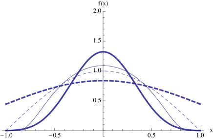
Figure 2: The wave function minimizing the variance $\phi_{1}$ (thin dashed), the rapidly decreasing function $g_{3}$ whose support is included in $[-1,1]$ (thin solid), prolate spheroidal wave function $\psi_{2}$ (thick dashed), and prolate spheroidal wave function $\psi_{10}$ (thick solid).

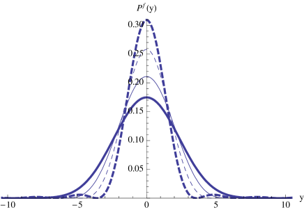
Figure 3: Probability density function minimizing variance $\mathrm{P}^{\phi_{1}}$ (thin dashed), probability density function improving tail probability $\mathrm{P}^{g_{3}}$ (thin solid), probability density function $\mathrm{P}^{\psi_{2}}$ (thick dashed), and probability density function $\mathrm{P}^{\psi_{10}}$ (thick solid).

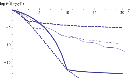
Figure 4: Logarithm of tail probabilities $\log\mathrm{P}^{\phi_{1}}([-y,y]^{c})$ (thin dashed), $\log\mathrm{P}^{g_{3}}([-y,y]^{c})$ (thin solid), $\log\mathrm{P}^{\psi_{2}}([-y,y]^{c})$ (thick dashed), $\log\mathrm{P}^{\psi_{10}}([-y,y]^{c})$ (thick solid), and Logarithm of the minimum tail probability $\log\min_{f\in L^{2}([-1,1])}\mathrm{P}^{f}([-y,y]^{c})$ (thick dotted).

Next, we generalize this problem slightly, i.e., we maximize the probability $\mathrm{P}^{f}([R_{1},R_{2}])$. In this case, the maximum value coincides with that of $\mathrm{P}^{f}([(R_{1}-R_{2})/2,(R_{2}-R_{1})/2])$, and its maximum is attained by the function $e^{ix(R_{1}+R_{2})/2}\psi_{(R_{2}-R_{1})/2}(x)$.

Since the function $R\mapsto\mathrm{P}^{f}([-R,R])$ is a strictly monotone increasing function, the inverse function $\beta\mapsto R(\beta)$ is a strictly monotone increasing function. Thus,

$$\min_{f\in L^{2}([-1,1])}\min\{R|\mathrm{P}^{f}([-R,R])\geq\beta\}=R(\beta).$$

Further, the LHS coincides with

$$\min_{f\in L^{2}([-1,1])}\min\{R|\mathrm{P}^{f}([-R+a,R+a])\geq\beta\}$$

for any real number $a$.

VI Interval estimation

Now, we treat the phase estimation problem with the interval estimation. In the interval estimation, given a confidence coefficient $\beta$, we estimate the confidence interval $[L,U]$, which the unknown parameter $\theta$ is guaranteed to belong to with the probability $\beta$. Here, since our parameter space is the torus $\mathbb{R}/2\pi\mathbb{Z}$, a careful treatment is required for the confidence interval $[L,U]$. That is, for $L,U\in[0,2\pi)$, the confidence interval $[L,U]$ is defined as a subset of $\mathbb{R}/2\pi\mathbb{Z}$ by

$$[L,U]:=\left\{\begin{array}[]{ll}[L,U]&\hbox{if }L<U\\ {[L,U+2\pi]}&\hbox{otherwise,}\end{array}\right.$$

and its width is defined

$$|[L,U]|:=\left\{\begin{array}[]{ll}U-L&\hbox{if }L<U\\ U+2\pi-L&\hbox{otherwise.}\end{array}\right.$$

In the interval estimation, the upper bound $U$ and the lower bound $L$ of the interval are chosen from the outcome $\omega$ obeying the distribution $\mathrm{P}_{\theta,\vec{a}}^{M}$. Since a smaller width $|[L(\omega),U(\omega)]|$ is better, we minimize the width $|[L(\omega),U(\omega)]|$ with the condition $\mathrm{P}_{\theta,\vec{a}}^{M}\{\omega|\theta\in[L(\omega),U(\omega)]\}\geq\beta$ for any $\theta\in[0,2\pi)$. That is, we consider

$$\min_{U,L,M,\vec{a}}\left\{\left.\max_{\omega}|[L(\omega),U(\omega)]|\right|\mathrm{P}_{\theta,\vec{a}}^{M}\{\omega|\theta\in[L(\omega),U(\omega)]\}\geq\beta,\quad\forall\theta\in[0,2\pi)\right\}$$ (14)

$$= \min_{U,L,M,\vec{a}}\max_{\theta\in[0,2\pi)}\left(\max_{\omega}\left\{|[L(\omega),U(\omega)]|\left|\mathrm{P}_{\theta,\vec{a}}^{M}\{\omega|\theta\in[L(\omega),U(\omega)]\}\geq\beta\right.\right\}\right)$$

The value (14) has a mini-max form of the cost $\max_{\omega}\left\{|[L(\omega),U(\omega)]|\left|\mathrm{P}_{\theta,\vec{a}}^{M}\{\omega|\theta\in[L(\omega),U(\omega)]\}\geq\beta\right.\right\}$, which has a covariant form. Thus, we can restrict our measurement into covariant measurement (2). Hence, our problem is reduced as

$$\min_{t,\vec{a}}\left(\max_{\omega}\left\{|[L(\omega),U(\omega)]|\left|\mathrm{P}_{\theta,\vec{a}}^{M}\{\omega|\theta\in[L(\omega),U(\omega)]\}\geq\beta\right.\right\}\right).$$

However, since it is quite difficult to treat this optimization with a finite $n$, we treat the following asymptotic setting as follows:

$$\lim_{n\to\infty}n\min_{t,\vec{a}}\left(\max_{\omega}\left\{|[L(\omega),U(\omega)]|\left|\mathrm{P}_{\theta,\vec{a}}^{M}\{\omega|\theta\in[L(\omega),U(\omega)]\}\geq\beta\right.\right\}\right)$$

$$= \min_{f\in L^{2}([-1,1])}\max_{\omega}\left\{|[L(\omega),U(\omega)]|\left|\mathrm{P}^{f}\left\{\omega|\theta\in[L(\omega),U(\omega)]\right\}\geq\beta\right.\right\}$$

$$= \min_{f\in L^{2}([-1,1])}\min\{2R|\mathrm{P}^{f}([-R,R])\geq\beta\}$$

$$= 2R(\beta).$$

This optimal value is attained when the input state constructed by the wave function $\psi_{R(\beta)}$ and the measurement is given by the covariant measurement (2) with the vector $|t_{0}\rangle$. That is, there exists a pair of functions $U$ and $L$ such that $|[L(\omega),U(\omega)]|\leq 2R(\beta)$ and $\mathrm{P}_{\theta,\vec{a}}^{M}\{\omega|\theta\in[L(\omega),U(\omega)]\}\geq\beta$. The optimal input state depends on the choice of the confidence coefficient $\beta$.

VII Continuous case with single copy

Let us consider the phase estimation in the continuous case with single copy, in which by inputing the wave function $f$, we estimate the parameter $\theta$ in a group-covariant model $\rho_{\theta}=e^{i\theta Q}\left|f\right>\left<f\right|e^{-i\theta Q}$ on the space $L^{2}(\mathbb{R})$.

It is known that when the shift-covariance condition is assumed for estimators, our estimator is restricted into the measurement of the observable $P$Holevo3 . Then, the outcome $\hat{\theta}$ obeys the distribution $\mathrm{P}^{f}$, and the variance of the outcome is given by $\left<f|\Delta P^{2}|f\right>$, which is abbreviated by $\langle\Delta P^{2}\rangle$.

If we can input any wave function $f$, the variance can be reduced infinitesimally. Hence, it is natural to assume a constraint for input wave function $f$. Here, we assume that the potential is given as a monotone function of the absolute value $|Q|$. While we often assume a constraint for average potential, we consider a deterministic condition for potential. That is, the wave packet of $f$ is assumed to exist only in the region where the potential is less than a given constant. In the following, for a simplicity for our analysis, we assume that the input wave function belongs to $L^{2}([-1,1])$. Hence, the discussion in Sections IV and V can be applied to this problem.

Here, it is meaningful to consider the relation with the Cramér-Rao bound. It is known in general that the Fisher information $J_{\theta}$ for a group-covariant model $\rho_{\theta}=e^{i\theta Q}\left|f\right>\left<f\right|e^{-i\theta Q}$ is given by $J_{\theta}=\left<\Delta Q^{2}\right>$ because the symmetric logarithmic derivative (SLD) is given by $Q-\left<Q\right>$Holevo3 .

Since the operator $P$ has a commutation relation with $Q$, we have the Heisenberg limit $\left<\Delta P^{2}\right>\left<\Delta Q^{2}\right>\geq 1/4$, which is equivalent with the Cramér-Rao inequality:

$$\left<\Delta P^{2}\right>\geq\frac{1}{4}J_{\theta}^{-1}.$$

Especially, if and only if $f$ is a squeezed state satisfying $\left<\Delta P^{2}\right>=c$ and $\left<\Delta Q^{2}\right>=c^{-1}$, the above inequality is achievable because its attainability is equivalent with that of $\left<\Delta P^{2}\right>\left<\Delta Q^{2}\right>\geq 1/4$. Thus, if $f$ is not a squeezed state, the Cramér-Rao lower bound $\frac{1}{4}J_{\theta}^{-1}$ cannot be attained uniformly in the one-copy case. As is shown in the next section, our asymptotic case is essentially equivalent to the above group-covariant model under the restriction of $\mathrm{supp}f\subset[-1,1]$.

VIII Asymptotic Cramér-Rao Lower Bound

Now, we consider the relation of our discussion with the Cramér-Rao lower bound because the Cramér-Rao approach is often employed in the asymptotic estimation of the unknown unitaryImai . When we apply the sequence of protocols ${\cal M}:=\{\vec{a}^{n}\}$, the phase estimation can be treated as the estimation problem in the state family $\{|\phi_{\theta,n}\rangle\langle\phi_{\theta,n}||\theta\in[0,2\pi]\}$, where $\left|\phi_{\theta,n}\right\rangle=\sum_{k=0}^{n}a_{k}^{n}e^{ik\theta}\left|k\right\rangle$. Let us calculate the SLD Fisher information. From the group covariance of the output state, it suffices to calculate the SLD Fisher information at $\theta=0$. Let $\left|l_{\theta,n}\right\rangle:=(1-\left|\phi_{\theta,n}\right\rangle\left\langle\phi_{\theta,n}\right|)\frac{\partial}{\partial\theta}\left|\phi_{\theta,n}\right\rangle$. The SLD Fisher information $J_{0,n}$ is given by $\frac{1}{4}J_{0,n}=\left\langle l_{0,n}\right|\left.l_{0,n}\right\rangle$.

$$\frac{J_{0,n}}{4} = \left\langle l_{0,n}\right|\left.l_{0,n}\right\rangle$$

$$= \left\langle\phi_{0,n}^{\prime}\right|\left.\phi_{0,n}^{\prime}\right\rangle-\left|\left\langle\phi_{0,n}\right|\left.\phi_{0,n}^{\prime}\right\rangle\right|^{2}$$

$$= \sum_{k=0}^{n}k^{2}\left|a_{k}^{n}\right|^{2}-\left(\sum_{k=0}^{n}k\left|a_{k}^{n}\right|^{2}\right)^{2}$$

where $\left|\phi_{0,n}^{\prime}\right\rangle=\left.\frac{\partial}{\partial\theta}\left|\phi_{\theta,n}\right\rangle\right|_{\theta=0}$. Choosing a smooth function $f_{n}$ by (8), we have

$$\frac{J_{0,n}}{4(n+1)^{2}}=\sum_{k=0}^{n}\left(x_{k}\right)^{2}\left|f_{n}(x_{k})\right|^{2}-\left(\sum_{k=0}^{n}\left(x_{k}\right)\left|f_{n}(x_{k})\right|^{2}\right)^{2}.$$

When $f_{n}$ converges to $f$,

$$\lim_{n\rightarrow\infty}\frac{J_{0,n}}{4(n+1)^{2}}= \int_{-1}^{1}x^{2}\left|f(x)\right|^{2}\mathrm{d}x-\left(\int_{-1}^{1}x\left|f(x)\right|^{2}\mathrm{d}x\right)^{2}$$

$$= \left\langle f\right|\Delta Q^{2}\left|f\right\rangle.$$

Since the variance of the limiting distribution is $\left\langle f\right|\Delta P^{2}\left|f\right\rangle$, we obtain the limiting distribution version of the Cramér-Rao inequality as

$$\left\langle f\right|\Delta P^{2}\left|f\right\rangle\geq\frac{1}{\lim_{n\rightarrow\infty}\frac{1}{4(n+1)^{2}}J_{0,n}}=\frac{1}{\left\langle f\right|\Delta Q^{2}\left|f\right\rangle}.$$

The equality holds if and only if the wave function $f$ is a squeezed state. However, since the support $f$ belongs to $[-1,1]$, the equality of the above cannot be attained. This fact indicates that the Cramer-Rao approach does not yield the attainable bound in the estimation of unitary action even in the asymptotic formulation, while this approach generally yields the attainable bound in the estimation of quantum state. This point is the essential difference between the state estimation and the unitary estimation.

IX Conclusion

As a unified approach to the asymptotic analysis on the phase estimation, we have treated the limiting distribution on the sequence of estimators because we can recover various asymptotic performance of the estimation protocols from the limiting distribution.

As the first step, we have found a one-to-one correspondence between a limiting distribution and a wave function on $L^{2}([-1,1])$. That is, we have shown that any limiting distribution is given by the absolute square of the Fourier transform of a wave function $f\in L^{2}([-1,1])$. Due to this correspondence, it is sufficient to optimize the distribution given as the square of the Fourier transform on $L^{2}([-1,1])$.

As the next step, the minimization of the variance has been treated among the above distributions by treating the Dirichlet problem in the similar way as Buzek et al Buzek . We have also considered its tail probability. In order to guarantee the small error probability out of the given interval, the limiting distribution is better to be rapidly decreasing. However, it has been clarified that the limiting distribution minimizing the variance is not rapidly decreasing. In order to construct such a limiting distribution, we employ a smoothing method so that we construct a rapidly decreasing function whose support is included in $[-1,1]$. It has been numerically checked that this function improves the tail probability remarkably.

Further, the tail probability for a given interval has been minimized among these limiting distribution by employing the Slepian and Pollak’s analysis on signal processingSlepianPollak . The optimal limiting distribution depends on the width of this interval. Using this optimization, we have treat the interval estimation in the asymptotic setting.

Next, we have treated the relation with the phase estimation in the continuous system with the one copy setting. In this case, the Heisenberg’s uncertainly relation is equivalent with Cramér-Rao inequality. Using this relation, we have obtained the condition for attainability of Cramér-Rao inequality. Further, we have applied this relation to the asymptotic analysis on the variance of the phase estimation. Then, we have clarified that the Cramér-Rao bound cannot be attained in our framework.

Throughout these discussions, it has been clarified that the optimization of asymptotic phase estimation cannot be characterized by a single parameter while this problem can be characterized by the single parameter, i.e., the variance, in the state estimation of a single parameter model with a regularity condition due to the asymptotic normalityGK ; GJK ; GJ . This property is the biggest difference from the state estimation.

Indeed, a similar property can be expected in a general unitary estimation. It is a future problem to investigate the limiting distribution in the estimation of unitary operation in a more general case.

Appendix A Elimination of multiplicity

The unitary $V_{\theta}^{\otimes n}$ can be written as the form

$$U_{\theta}^{\prime}=\sum_{k=0}^{n}\sum_{j=1}^{m_{k}}e^{i(k-\frac{n}{2})\theta}\left|k,j\right\rangle\left\langle k,j\right|$$

with the multiplicity $m_{k}={n\choose k}$. When the unitary $U_{\theta}^{\prime}$ acts on the input state $\sum_{k=0}^{n}\sum_{j=1}^{m_{k}}a_{k,j}\left|k,j\right\rangle$, the final state is given by $\sum_{k=0}^{n}\sum_{j=1}^{m_{k}}e^{i(k-\frac{n}{2})\theta}a_{k,j}\left|k,j\right\rangle=\sum_{k=0}^{n}e^{i(k-\frac{n}{2})\theta}(\sum_{j=1}^{m_{k}}a_{k,j}\left|k,j\right\rangle)=\sum_{k=0}^{n}e^{i(k-\frac{n}{2})\theta}a_{k}\left|k\right\rangle)$ where $a_{k}:=\sqrt{\sum_{j=1}^{m_{k}}|a_{k,j}|^{2}}$ and $\left|k\right\rangle:=\frac{1}{a_{k}}\sum_{j=1}^{m_{k}}a_{k,j}\left|k,j\right\rangle$. Then, the estimation problem of $U_{\theta}^{\prime}$ can be reduced in that of $U_{\theta}$ given in (1).

Appendix B Proof of (12)

Now, we prove (12). Assume that $y>0$. For a given integer $N$,s

$$\frac{\sqrt{2\pi}}{C}|\int_{-\infty}^{\infty}F(g_{1})(y^{\prime})F(g_{2})(y-y^{\prime})dy^{\prime}|$$

$$\leq \sum_{k=1}^{N}\frac{\sqrt{2\pi}}{C}\max_{y^{\prime}\in[y\frac{k-1}{N},y\frac{k}{N}]}|F(g_{1})(y^{\prime})|\cdot|F(g_{2})(y-y^{\prime})|\frac{y}{N}$$

$$+\frac{\sqrt{2\pi}}{C}\int_{-\infty}^{0}|F(g_{1})(y^{\prime})|\cdot|F(g_{2})(y-y^{\prime})|dy^{\prime}$$

$$+\frac{\sqrt{2\pi}}{C}\int_{y}^{\infty}|F(g_{1})(y^{\prime})|\cdot|F(g_{2})(y-y^{\prime})|dy^{\prime}.$$

Since $|F(g_{1})(y^{\prime})|$ is bounded,

$$\frac{\sqrt{2\pi}}{C}\int_{-\infty}^{0}|F(g_{1})(y^{\prime})|\cdot|F(g_{2})(y-y^{\prime})|dy^{\prime}$$

$$\cong O(\int_{-\infty}^{0}|F(g_{2})(y-y^{\prime})|dy^{\prime})\cong O(e^{-\sqrt{2}\sqrt{y}}).$$

Similarly,

$$\frac{\sqrt{2\pi}}{C}\int_{y}^{\infty}|F(g_{1})(y^{\prime})|\cdot|F(g_{2})(y-y^{\prime})|dy^{\prime}\cong O(e^{-\sqrt{2}\sqrt{y}}).$$

Further,

$$\frac{\sqrt{2\pi}}{C}\max_{y^{\prime}\in[y\frac{k-1}{N},y\frac{k}{N}]}|F(g_{1})(y^{\prime})|\cdot|F(g_{2})(y-y^{\prime})|\frac{y}{N}$$

$$\cong O(e^{-\sqrt{2}\sqrt{y\frac{k-1}{N}}}\cdot e^{-\sqrt{2}\sqrt{y-y\frac{k}{N}}})\leq O(e^{-\sqrt{2}\sqrt{y(1-\frac{1}{N}})}).$$

Therefore,

$$\frac{\sqrt{2\pi}}{C}|\int_{-\infty}^{\infty}F(g_{1})(y^{\prime})F(g_{2})(y-y^{\prime})dy^{\prime}| \leq O(e^{-\sqrt{2}\sqrt{y(1-\frac{1}{N}})}).$$

Since $N$ is arbitrary,

$$\frac{\sqrt{2\pi}}{C}|\int_{-\infty}^{\infty}F(g_{1})(y^{\prime})F(g_{2})(y-y^{\prime})dy^{\prime}| \leq O(e^{-\sqrt{2}\sqrt{y}}).$$

Taking the square, we obtain (12).

In the case of $y<0$, we can show (12) by replacing $y^{\prime}$ by $-y^{\prime}$.

References

- (1) R. Cleve, A. Ekert, C. Macchiavello and M. Mosca, “Quantum Algorithm Revisited,” Proc. R. Soc. London, Ser. A 454, 339, 1998.
- (2) A. Y. Kitaev, A. H. Shen and M. N. Vyalyi, Classical and Quantum Computation, (Graduate Studies in Mathematics 47), Americal Mathematical Society, 2002.
- (3) V. Giovannetti, S. Lloyd and L. Maccone, “Quantum-enhanced measurements: beating the standard quantum limit,” Science 306, 1330-1336, 2004.
- (4) V. Buzek, R. Derka and S. Massar, “Optimal Quantum Clocks,” Phys. Rev. Lett. 82 (1999) 2207, quant-ph/9808042.
- (5) M. Hayashi, “Parallel Treatment of Estimation of SU(2) and Phase Estimation,” Phys. Lett. A 354, 183-189, 2006.
- (6) H. Imai and A. Fujiwara, “Geometry of optimal estimation scheme for SU(D) channels,” J. Phys. A 40, 4391-4400, 2007.
- (7) B. L. Higgins, D. W. Berry, S. D. Bartlett, H. M. Wiseman and G. J. Pryde, “Entanglement-free Heisenberg-limited phase estimation,” Nature 450, 393-396, 2007.
- (8) A. Y. Kitaev, “Quantum Computations: Algorithms and Error Correction,” Russ. Math. Surv. 52, 1191-1249, 1997.
- (9) M. Hayashi and K. Matsumoto, “Asymptotic performance of optimal state estimation in quantum two level system,” quant-ph/0411073.
- (10) M. Guţă and J. Kahn, “Local asymptotic normality for qubit states,” Phys. Rev. A, 73, 052108 (2006).
- (11) M. Guţă, B. Janssens, and J. Kahn, “Optimal estimation of qubit states with continuous time measurements,” Commun. Math. Phys., 277, 127-160 (2008).
- (12) M. Guţă and A. Jencova, “Local asymptotic normality in quantum statistics,” Commun. Math. Phys., 276, 341-379 (2007).
- (13) D. Pope, H. M. Wiseman and N. K. Langford, “Adaptive Phase estimation is more accurate than nonadaptive phase estimation for continuous beams of light,” Phys. Rev. A A70, 043812-1 - 043812-13 2004.
- (14) R. J. Larsen and M. L. Marx, An Introduction to Mathematical Statistics and Its Applications, Pearson Education, U.S., 2005.
- (15) D. Slepian and H. O. Pollak, “Prolate spheroidal wave functions, Fourier analysis and uncertainty-I,” Bell Syst. Tech. J., 40, 43-63, 1961.
- (16) D. Slepian, “Some asymptotic expansions for prolate spheroidal functions,” J. Math. Phys. 44, 99–140, 1965.
- (17) L. Li, M. Leong, T. Yeo and Y. Gan, “Electromagnetic radiation from a prolate spheroidal antenna enclosed in a confocal spheroidal radome,” IEEE Trans. on Antenn. and Propa., 50, 1525-1533, 2002.
- (18) P. Nazmi, P. Kapadia and J. Dowden, “A mathematical model of heat conduction in a prolate spheroidal coordinate system with applications to the theory of welding,” J. Phys. D, 26, 563-573, 1993.
- (19) A. S. Holevo, “Covariant Measurements and Uncertainty Relations,” Rep. Math. Phys. 16, 385-400, 1979.
- (20) E. A. Coddington and N. Levinson, Theory of differential equations, McGraw-Hill, New-York, 1955.
- (21) F. P. Kelly (ed.), Probability, Statistics and Optimization: A Tribute to Peter Whittle (Wiley Series in Probability and Statistics), John Wiley & Sons Inc., 1994.
- (22) A. S. Holevo, “Asymptotic estimation of shift parameter of a quantum state,” quant-ph/0307225.
- (23) A. S. Holevo, Probabilistic and Statistical Aspects of Quantum Theory, (North-Holland, Amsterdam, 1982); Originally published in Russian (1980).
- (24) W. van Dam, G. M. D’Ariano, A. Ekert, C. Macchiavello, and M. Mosca, “Optimal quantum circuits for general phase estimation,” quant-ph/0609160.