The Pentagram map: a discrete integrable system

Abstract

The pentagram map is a projectively natural transformation defined on (twisted) polygons. A twisted polygon is a map from ${\mathbb{Z}}$ into ${\mathbb{RP}}^{2}$ that is periodic modulo a projective transformation called the monodromy. We find a Poisson structure on the space of twisted polygons and show that the pentagram map relative to this Poisson structure is completely integrable. For certain families of twisted polygons, such as those we call universally convex, we translate the integrability into a statement about the quasi-periodic motion for the dynamics of the pentagram map. We also explain how the pentagram map, in the continuous limit, corresponds to the classical Boussinesq equation. The Poisson structure we attach to the pentagram map is a discrete version of the first Poisson structure associated with the Boussinesq equation. A research announcement of this work appeared in [16].

1 Introduction

The notion of integrability is one of the oldest and most fundamental notions in mathematics. The origins of integrability lie in classical geometry and the development of the general theory is always stimulated by the study of concrete integrable systems. The purpose of this paper is to study one particular dynamical system that has a simple and natural geometric meaning and to prove its integrability. Our main tools are mostly geometric: the Poisson structure, first integrals and the corresponding Lagrangian foliation. We believe that our result opens doors for further developments involving other approaches, such as Lax representation, algebraic-geometric and complex analysis methods, Bäcklund transformations; we also expect further generalizations and relations to other fields of modern mathematics, such as cluster algebras theory.

The pentagram map, $T$, was introduced in [19], and further studied in [20] and [21]. Originally, the map was defined for convex closed $n$-gons. Given such an $n$-gon $P$, the corresponding $n$-gon $T(P)$ is the convex hull of the intersection points of consequtive shortest diagonals of $P$. Figure 1 shows the situation for a convex pentagon and a convex hexagon. One may consider the map as defined either on unlabelled polygons or on labelled polygons. Later on, we shall consider the labelled case in detail.

Figure 1: The pentagram map defined on a pentagon and a hexagon

The pentagram map already has some surprising features in the cases $n=5$ and $n=6$. When $P$ is a pentagon, there is a projective transformation carrying $P$ to $T(P)$. This is a classical result, cf. [15]; one of us learned of this result from John Conway in $1987$. When $P$ is a hexagon, there is a projective transformation carrying $P$ to $T^{2}(P)$. It is not clear whether this result was well-known to classical projective geometers, but it is easy enough to prove. The name pentagram map stems from the fact that the pentagon is the simplest kind of polygon for which the map is defined.

Letting ${\cal C\/}_{n}$ denote the space of convex $n$-gons modulo projective transformations, we can say that the pentagram map is periodic on ${\cal C\/}_{n}$ for $n=5,6$. The pentagram map certainly is not periodic on ${\cal C\/}_{n}$ for $n\geq 7$. Computer experiments suggest that the pentagram map on ${\cal C\/}_{n}$ in general displays the kind of quasi-periodic motion one sees in completely integrable systems. Indeed, this was conjectured (somewhat loosely) in [21]. See the remarks following Theorem 1.2 in [21].

It is the purpose of this paper to establish the complete integrability conjectured in [21] and to explain the underlying quasi-periodic motion. However, rather than work with closed $n$-gons, we will work with what we call twisted $n$-gons. A twisted $n$-gon is a map $\phi:{\mathbb{Z}}\to{\mathbb{RP}}^{2}$ such that that

$$\phi(k+n)=M\circ\phi(k);\hskip 10.0pt\forall k.$$

Here $M$ is some projective automorphism of ${\mathbb{RP}}^{2}$. We call $M$ the monodromy. For technical reasons, we require that every $3$ consecutive points in the image are in general position – i.e., not collinear. When $M$ is the identity, we recover the notion of a closed $n$-gon. Two twisted $n$-gons $\phi_{1}$ and $\phi_{2}$ are equivalent if there is some projective transformation $\Psi$ such that $\Psi\circ\phi_{1}=\phi_{2}$. The two monodromies satisfy $M_{2}=\Psi M_{1}\Psi^{-1}$. Let ${\mathcal{P}}_{n}$ denote the space of twisted $n$-gons modulo equivalence.

Let us emphasise that the full space of twisted $n$-gons (rather than the geometrically natural but more restricted space of closed $n$-gons) is much more natural in the general context of the integrable systems theory. Indeed, in the “smooth case” it is natural to consider the full space of linear differential equations; the monodromy then plays an essential rôle in producing the invariants. This viewpoint is adopted by many authors (see [9, 14] and references therein) and this is precisely our viewpoint in the discrete case.

The pentagram map is generically defined on ${\mathcal{P}}_{n}$. However, the lack of convexity makes it possible that the pentagram map is not defined on some particular point of ${\mathcal{P}}_{n}$, or that the image of a point in ${\mathcal{P}}_{n}$ under the pentagram map no longer belongs to ${\mathcal{P}}_{n}$. That is, we can lose the $3$-in-a-row property that characterizes twisted polygons. We will put coordinates in ${\mathcal{P}}_{n}$ so that the pentagram map becomes a rational map. At least when $n$ is not divisible by $3$, the space ${\mathcal{P}}_{n}$ is diffeomorphic to ${\mathbb{R}}^{2n}$. When $n$ is divisible by $3$, the topology of the space is trickier, but nonetheless large open subsets of ${\mathcal{P}}_{n}$ in this case are still diffeomorphic to open subsets of ${\mathbb{R}}^{2n}$. (Since our map is only generically defined, the fine points of the global topology of ${\mathcal{P}}_{n}$ are not so significant.)

The action of the pentagram map in ${\mathcal{P}}_{n}$ was studied extensively in [21]. In that paper, it was shown that for every $n$ this map has a family of invariant functions, the so-called weighted monodromy invariants. There are exactly $2[n/2]+2$ algebraically independent invariants. Here $[n/2]$ denotes the floor of $n/2$. When $n$ is odd, there are two exceptional monodromy functions that are somewhat unlike the rest. When $n$ is even, there are $4$ such exceptional monodromy functions. We will recall the explicit construction of these invariants in the next section, and sketch the proofs of some of their properties. Later on in the paper, we shall give a new treatment of these invariants.

Here is the main result of this paper.

Theorem 1

There exists a Poisson structure on ${\mathcal{P}}_{n}$ having co-rank $2$ when $n$ is odd and co-rank $4$ when $n$ is even. The exceptional monodromy functions generically span the null space of the Poisson structure, and the remaining monodromy invariants Poisson-commute. Finally, the Poisson structure is invariant under the pentagram map.

The exceptional monodromy functions are precisely the Casimir functions for the Poisson structure. The generic level set of the Casimir functions is a smooth symplectic manifold. Indeed, as long as we keep all the values of the Casimir functions nonzero, the corresponding level sets are smooth symplectic manifolds. The remaining monodromy invariants, when restricted to the symplectic level sets, define a singular Lagrangian foliation. Generically, the dimension of the Lagrangian leaves is precisely the same as the number of remaining monodromy invariants. This is the classical picture of Arnold-Liouville complete integrability.

As usual in this setting, the complete integrability gives an invariant affine structure to every smooth leaf of the Lagrangian foliation. Relative to this structure, the pentagram map is a translation. Hence

Corollary 1.1

Suppose that $P$ is a twisted $n$-gon that lies on a smooth Lagrangian leaf and has a periodic orbit under the pentagram map. If $P^{\prime}$ is any twisted $n$-gon on the same leaf, then $P^{\prime}$ also has a periodic orbit with the same period, provided that the orbit of $P^{\prime}$ is well-defined.

Remark 1.2

In the result above, one can replace the word periodic with ${\varepsilon}$-periodic. By this we mean that we fix a Euclidean metric on the leaf and measure distances with respect to this metric.

We shall not analyze the behavior of the pentagram map on ${\cal C\/}_{n}$. One of the difficulties in analyzing the space ${\cal C\/}_{n}$ of closed convex polygons modulo projective transformations is that this space has positive codimension in ${\mathcal{P}}_{n}$ (codimension 8). We do not know in enough detail how the Lagrangian singular foliation intersects ${\cal C\/}_{n}$, and so we cannot appeal to the structure that exists on generic leaves. How the monodromy invariants behave when restricted to ${\cal C\/}_{n}$ is a subtle and interesting question that we do not yet fully know how to answer (see Theorem 4 for a partial result). We hope to tackle the case of closed $n$-gons in a sequel paper.

One geometric setting where our machine works perfectly is the case of universally convex $n$-gons. This is our term for a twisted $n$-gon whose image in ${\mathbb{RP}}^{2}$ is strictly convex. The monodromy of a universally convex $n$-gon is necessarily an element of $PGL_{3}({\mathbb{R}})$ that lifts to a diagonalizable matrix in $SL_{3}({\mathbb{R}})$. A universally convex polygon essentially follows along one branch of a hyperbola-like curve. Let ${\cal U\/}_{n}$ denote the space of universally convex $n$-gons, modulo equivalence. We will prove that ${\cal U\/}_{n}$ is an open subset of ${\cal P\/}_{n}$ locally diffeomorphic to ${\mathbb{R}}^{2n}$. Further, we will see that the pentagram map is a self-diffeomorphism of ${\cal U\/}^{2n}$. Finally, we will see that every leaf in the Lagrangian foliation intersects ${\cal U\/}_{n}$ in a compact set.

Combining these results with our Main Theorem and some elementary differential topology, we arrive at the following result.

Theorem 2

Almost every point of ${\cal U\/}_{n}$ lies on a smooth torus that has a $T$-invariant affine structure. Hence, the orbit of almost every universally convex $n$-gon undergoes quasi-periodic motion under the pentagram map.

We will prove a variant of Theorem 2 for a different family of twisted $n$-gons. See Theorem 3. The general idea is that certain points of ${\mathcal{P}}_{n}$ can be interpreted as embedded, homologically nontrivial, locally convex polygons on projective cylinders, and suitable choices of geometric structure give us the compactness we need for the proof.

Here we place our results in a context. First of all, it seems that there is some connection between our work and cluster algebras. On the one hand, the space of twisted polygons is known as an example of cluster manifold, see [7, 6] and discussion in the end of this paper. This implies in particular that ${\mathcal{P}}_{n}$ is equipped with a canonical Poisson structure, see [10]. We do not know if the Poisson structure constructed in this paper coincides with the canonical cluster Poisson structure. On the other hand, it was shown in [21] that a certain change of coordinates brings the pentagram map rather closely in line with the octahedral recurrence, which is one of the prime examples in the theory of cluster algebras, see [18, 11, 22].

Second of all, there is a close connection between the pentagram map and integrable P.D.E.s. In the last part of this paper we consider the continuous limit of the pentagram map. We show that this limit is precisely the classical Boussinesq equation which is one of the best known infinite-dimensional integrable systems. Moreover, we argue that the Poisson bracket constructed in the present paper is a discrete analog of so-called first Poisson structure of the Boussinesq equation. We remark that a connection to the Boussinesq equation was mentioned in [19], but no derivation was given.

Discrete integrable systems is an actively developing subject, see, e.g., [26] and the books [23, 5]. The paper [4] discusses a well-known discrete version (but with continuous time) of the Boussinesq equation; see [25] (and references therein) for a lattice version of this equation. See [9] (and references therein) for a general theory of integrable difference equations. Let us stress that the $r$-matrix Poisson brackets considered in [9] are analogous to the second (i.e., the Gelfand-Dickey) Poisson bracket. A geometric interpretation of all the discrete integrable systems considered in the above references is unclear.

In the geometrical setting which is more close to our viewpoint, see [5] for many interesting examples. The papers [1, 2] considers a discrete integrable systems on the space of $n$-gons, different from the pentagram map. The recent paper [13] considers a discrete integrable systems in the setting of projective differential geometry; some of the formulas in this paper are close to ours. Finally, we mention [12, 14] for discrete and continuous integrable systems related both to Poisson geometry and projective differential geometry on the projective line.

We turn now to a description of the contents of the paper. Essentially, our plan is to make a bee-line for all our main results, quoting earlier work as much as possible. Then, once the results are all in place, we will consider the situation from another point of view, proving many of the results quoted in the beginning.

One of the disadvantages of the paper [21] is that many of the calculations are ad hoc and done with the help of a computer. Even though the calculations are correct, one is not given much insight into where they come from. In this paper, we derive everything in an elementary way, using an analogy between twisted polygons and solutions to periodic ordinary differential equations.

One might say that this paper is organized along the lines of first the facts, then the reasons. Accordingly, there is a certain redundancy in our treatment. For instance, we introduce two natural coordinate systems in ${\mathcal{P}}_{n}$. In the first coordinate system, which comes from [21], most of the formulas are simpler. However, the second coordinate system, which is new, serves as a kind of engine that drives all the derivations in both coordinate systems; this coordinate system is better for computation of the monodromy too. Also, we discovered the invariant Poisson structure by thinking about the second coordinate system.

In §2 we introduce the first coordinate system, describe the monodromy invariants, and establish the Main Theorem. In §3 we apply the main theorem to universally convex polygons and other families of twisted polygons. In §4 we introduce the second coordinate system. In §4 and 5 we use the second coordinate system to derive many of the results we simply quoted in §2. Finally, in §6 we use the second coordinate system to derive the continuous limit of the pentagram map.

2 Proof of the Main Theorem

2.1 Coordinates for the space

In this section, we introduce our first coordinate system on the space of twisted polygons. As we mentioned in the introduction, a twisted $n$-gon is a map $\phi:{\mathbb{Z}}\to{\mathbb{RP}}^{2}$ such that

$$\phi(n+k)=M\circ\phi(k)$$ (2.1)

for some projective transformation $M$ and all $k$. We let $v_{i}=\phi(i)$. Thus, the vertices of our twisted polygon are naturally $...v_{i-1},v_{i},v_{i+1},...$. Our standing assumption is that $v_{i-1},v_{i},v_{i+1}$ are in general position for all $i$, but sometimes this assumption alone will not be sufficient for our constructions.

The cross ratio is the most basic invariant in projective geometry. Given four points $t_{1},t_{2},t_{3},t_{4}\in{\mathbb{RP}}^{1}$, the cross-ratio $[t_{1},t_{2},t_{3},t_{4}]$ is their unique projective invariant. The explicit formula is as follows. Choose an arbitrary affine parameter, then

$$[t_{1},t_{2},t_{3},t_{4}]=\frac{(t_{1}-t_{2})\,(t_{3}-t_{4})}{(t_{1}-t_{3})\,(t_{2}-t_{4})}.$$ (2.2)

This expression is independent of the choice of the affine parameter, and is invariant under the action of ${\mathrm{PGL}}(2,{\mathbb{R}})$ on ${\mathbb{RP}}^{1}$.

Remark 2.1

Many authors define the cross ratio as the multiplicative inverse of the formula in Equation 2.2. Our definition, while perhaps less common, better suits our purposes.

The cross-ratio was used in [21] to define a coordinate system on the space of twisted $n$-gons. As the reader will see from the definition, the construction requires somewhat more than $3$ points in a row to be in general position. Thus, these coordinates are not entirely defined on our space ${\mathcal{P}}_{n}$. However, they are generically defined on our space, and this is sufficient for all our purposes.

The construction is as follows, see Figure 2. We associate to every vertex $v_{i}$ two numbers:

$$\begin{array}[]{rcl}x_{i}&=&\displaystyle\left[v_{i-2},\,v_{i-1},\,\left((v_{i-2},v_{i-1})\cap(v_{i},v_{i+1})\right),\,\left((v_{i-2},v_{i-1})\cap(v_{i+1},v_{i+2})\right)\right]\\[10.0pt] y_{i}&=&\displaystyle[\left((v_{i-2},v_{i-1})\cap(v_{i+1},v_{i+2})\right),\,\left((v_{i-1},v_{i})\cap(v_{i+1},v_{i+2})\right),\,v_{i+1},\,v_{i+2}]\end{array}$$ (2.3)

called the left and right corner cross-ratios. We often call our coordinates the corner invariants.

Figure 2: Points involved in the definition of the invariants

Clearly, the construction is ${\mathrm{PGL}}(3,{\mathbb{R}})$-invariant and, in particular, $x_{i+n}=x_{i}$ and $y_{i+n}=y_{i}$. We therefore obtain a (local) coordinate system that is generically defined on the space ${\mathcal{P}}_{n}$. In [21], §4.2, we show how to reconstruct a twisted $n$-gon from its sequence of invariants. The reconstruction is only canonical up to projective equivalence. Thus, an attempt to reconstruct $\phi$ from $x_{1},y_{1},...$ perhaps would lead to an unequal but equivalent twisted polygon. This does not bother us. The following lemma is nearly obvious.

Lemma 2.2

At generic points, the space ${\mathcal{P}}_{n}$ is locally diffeomorphic to ${\mathbb{R}}^{2n}$.

Proof.

We can perturb our sequence $x_{1},y_{1},...$ in any way we like to get a new sequence $x_{1}^{\prime},y_{1}^{\prime},...$. If the perturbation is small, we can reconstruct a new twisted $n$-gon $\phi^{\prime}$ that is near $\phi$ in the following sense. There is a projective transformation $\Psi$ such that $n$-consecutive vertices of $\Psi(\phi^{\prime})$ are close to the corresponding $n$ consecutive vertices of $\phi$. In fact, if we normalize so that a certain quadruple of consecutive points of $\Psi(\phi^{\prime})$ match the corresponding points of $\phi$, then the remaining points vary smoothly and algebraically with the coordinates. The map $(x_{1}^{\prime},y_{2}^{\prime},...,x_{n}^{\prime},y_{n}^{\prime})\to[\phi^{\prime}]$ (the class of $\phi^{\prime}$) gives the local diffeomorphism. $\Box$

Remark 2.3

(i) Later on in the paper, we will introduce new coordinates on all of ${\mathcal{P}}_{n}$ and show, with these new coordinates, that ${\mathcal{P}}_{n}$ is globally diffeomorphic to ${\mathbb{R}}^{2n}$ when $n$ is not divisible by $3$.
(ii) The actual lettering we use here to define our coordinates is different from the lettering used in [21]. Here is the correspondense:

$$...p_{1},q_{2},p_{3},q_{4}...\hskip 30.0pt\Longleftrightarrow\hskip 30.0pt...,x_{1},y_{1},x_{2},y_{2},...$$

2.2 A formula for the map

In this section, we express the pentagram map in the coordinates we have introduced in the previous section. To save words later, we say now that we will work with generic elements of ${\mathcal{P}}_{n}$, so that all constructions are well-defined. Let $\phi\in{\mathcal{P}}_{n}$. Consider the image, $T(\phi)$, of $\phi$ under the pentagram map. One difficulty in making this definition is that there are two natural choices for labelling $T(\phi)$, the left choice and the right choice. These choices are shown in Figure 3. In the picture, the black dots represent the vertices of $\phi$ and the white dots represent the vertices of $T(\phi)$. The labelling continues in the obvious way.

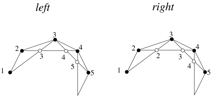
Figure 3: Left and right labelling schemes

If one considers the square of the pentagram map, the difficulty in making this choice goes away. However, for most of our calculations it is convenient for us to arbitrarily choose right over left and consider the pentagram map itself and not the square of the map. Henceforth, we make this choice.

Lemma 2.4

Suppose the coordinates for $\phi$ are $x_{1},y_{1},...$ then the coordinates for $T(\phi)$ are

$$T^{*}x_{i}=x_{i}\,\frac{1-x_{i-1}\,y_{i-1}}{1-x_{i+1}\,y_{i+1}},\qquad T^{*}y_{i}=y_{i+1}\,\frac{1-x_{i+2}\,y_{i+2}}{1-x_{i}\,y_{i}},$$ (2.4)

where $T^{*}$ is the standard pull-back of the (coordinate) functions by the map $T$.

In [21], Equation 7, we express the squared pentagram map as the product of two involutions on ${\mathbb{R}}^{2n}$, and give coordinates. From this equation one can deduce the formula in Lemma 2.4 for the pentagram map itself. Alternatively, later in the paper we will give a self-contained proof of Lemma 2.4.

Lemma 2.4 has two corollaries, which we mention here. These corollaries are almost immediate from the formula. First, there is an interesting scaling symmetry of the pentagram map. We have a rescaling operation on ${\mathbb{R}}^{2n}$, given by the expression

$$R_{t}:\hskip 10.0pt(x_{1},y_{1},...,x_{n},y_{n})\to(tx_{1},t^{-1}y_{1},...,tx_{n},t^{-1}y_{n}).$$ (2.5)

Corollary 2.5

The pentagram map commutes with the rescaling operation.

Second, the formula for the pentagram map exhibits rather quickly some invariants of the pentagram map. When $n$ is odd, define

$$O_{n}=\prod_{i=1}^{n}x_{i};\hskip 30.0ptE_{n}=\prod_{i=1}^{n}y_{i}.$$ (2.6)

When $n$ is even, define

$$O_{n/2}=\prod_{i\ {\rm even\/}}x_{i}+\prod_{i\ {\rm odd\/}}x_{i},\hskip 20.0ptE_{n/2}=\prod_{i\ {\rm even\/}}y_{i}+\prod_{i\ {\rm odd\/}}y_{i}.$$ (2.7)

The products in this last equation run from $1$ to $n$.

Corollary 2.6

When $n$ is odd, the functions $O_{n}$ and $E_{n}$ are invariant under the pentagram map. When $n$ is even, the functions $O_{n/2}$ and $E_{n/2}$ are also invariant under the pentagram map.

These functions are precisely the exceptional invariants we mentioned in the introduction. They turn out to be the Casimirs for our Poisson structure.

2.3 The monodromy invariants

In this section we introduce the invariants of the pentagram map that arise in Theorem 1.

The invariants of the pentagram map were defined and studied in [21]. In this section we recall the original definition. Later on in the paper, we shall take a different point of view and give self-contained derivations of everything we say here.

As above, let $\phi$ be a twisted $n$-gon with invariants $x_{1},y_{1},...$. Let $M$ be the monodromy of $\phi$. We lift $M$ to an element of $GL_{3}({\mathbb{R}})$. By slightly abusing notation, we also denote this matrix by $M$. The two quantities

$$\Omega_{1}=\frac{{\rm trace\/}^{3}(M)}{{\rm det\/}(M)};\hskip 40.0pt\Omega_{2}=\frac{{\rm trace\/}^{3}(M^{-1})}{{\rm det\/}(M^{-1})};$$ (2.8)

enjoy $3$ properties.

• $\Omega_{1}$ and $\Omega_{2}$ are independent of the lift of $M$.

• $\Omega_{1}$ and $\Omega_{2}$ only depend on the conjugacy class of $M$.

• $\Omega_{1}$ and $\Omega_{2}$ are rational functions in the corner invariants.

We define

$$\widetilde{\Omega}_{1}=O_{n}^{2}E_{n}\Omega_{1};\hskip 30.0pt\widetilde{\Omega}_{2}=O_{n}E_{n}^{2}\Omega_{2}.$$ (2.9)

In [21] it is shown that $\widetilde{\Omega}_{1}$ and $\widetilde{\Omega}_{2}$ are polynomials in the corner invariants. Since the pentagram map preserves the monodromy, and $O_{n}$ and $E_{n}$ are invariants, the two functions $\widetilde{\Omega}_{1}$ and $\widetilde{\Omega}_{2}$ are also invariants.

We say that a polynomial in the corner invariants has weight $k$ if we have the following equation

$$R_{t}^{*}(P)=t^{k}P.$$ (2.10)

here $R_{t}^{*}$ denotes the natural operation on polynomials defined by the rescaling operation (2.5). For instance, $O_{n}$ has weight $n$ and $E_{n}$ has weight $-n$. In [21] it is shown that

$$\widetilde{\Omega}_{1}=\sum_{k=1}^{[n/2]}O_{k};\hskip 30.0pt\widetilde{\Omega}_{2}=\sum_{k=1}^{[n/2]}E_{k}$$ (2.11)

where $O_{k}$ has weight $k$ and $E_{k}$ has weight $-k$. Since the pentagram map commutes with the rescaling operation and preserves $\widetilde{\Omega}_{1}$ and $\widetilde{\Omega}_{2}$, it also preserves their “weighted homogeneous parts”. That is, the functions $O_{1},E_{1},O_{2},E_{2},...$ are also invariants of the pentagram map. These are the monodromy invariants. They are all nontrivial polynomials.

Algebraic Independence: In [21], §6, it is shown that the monodromy invariants are algebraically independent provided that, in the even case, we ignore $O_{n/2}$ and $E_{n/2}$. We will not reproduce the proof in this paper, so here we include a brief description of the argument. Since we are mainly trying to give the reader a feel for the argument, we will explain a variant of the method in [21]. Let $f_{1},...,f_{k}$ be the complete list of invariants we have described above. Here $k=2[n/2]+2$. If our functions were not algebraically independent, then the gradients $\nabla f_{1},...,\nabla f_{k}$ would never be linearly independent. To rule this out, we just have to establish the linear independence at a single point. One can check this at the point $(1,\omega,...,\omega^{2n})$, where $\omega$ is a $(4n)$th root of unity. The actual method in [21] is similar to this, but uses a trick to make the calculation easier. Given the formulas for the invariants we present below, this calculation is really just a matter of combinatorics. Perhaps an easier calculation can be made for the point $(0,1,...,1)$, which also seems to work for all $n$.

2.4 Formulas for the invariants

In this section, we recall the explicit formulas for the monodromy invariants given in [21]. Later on in the paper, we will give a self-contained derivation of the formulas. From the point of view of our main theorems, we do not need to know the formulas, but only their algebraic independence and Lemma 2.8 below.

We introduce the monomials

$$X_{i}:=x_{i}\,y_{i}\,x_{i+1}.$$ (2.12)

1. We call two monomials $X_{i}$ and $X_{j}$ consecutive if $j\in\left\{i-2,\,i-1,\,i,\,i+1,\,i+2\right\};$

2. we call $X_{i}$ and $x_{j}$ consecutive if $j\in\left\{i-1,\,i,\,i+1,\,i+2\right\};$

3. we call $x_{i}$ and $x_{i+1}$ consecutive.

Let $O(X,x)$ be a monomial obtained by the product of the monomials $X_{i}$ and $x_{j}$, i.e.,

$$O=X_{i_{1}}\cdots{}X_{i_{s}}\,x_{j_{1}}\cdots{}x_{j_{t}}.$$

Such a monomial is called admissible if no two of the indices are consecutive. For every admissible monomial, we define the weight $|O|$ and the sign $\mathrm{sign}(O)$ by

$$|O|:=s+t,\qquad\mathrm{sign}(O):=(-1)^{t}.$$

With these definitions, it turns out that

$$O_{k}=\sum_{|O|=k}\mathrm{sign}(O)\,O;\hskip 30.0ptk\in\left\{1,2,\ldots,\left[\frac{n}{2}\right]\right\}$$ (2.13)

The same formula works for $E_{k}$, if we make all the same definitions with $x$ and $y$ interchanged.

Example 2.7

For $n=5$ one obtains the following polynomials

$$O_{1}=\sum_{i=1}^{5}\left(x_{i}\,y_{i}\,x_{i+1}-x_{i}\right),\qquad O_{2}=\sum_{i=1}^{5}\left(x_{i}\,x_{i+2}-x_{i}\,y_{i}\,x_{i+1}\,x_{i+3}\right)$$

together with $O_{5}$.

Now we mention the needed symmetry property. Let $\tau$ be the involution on the indices:

$$\tau:{}\left\{\begin{array}[]{l}x_{i}\mapsto x_{1-i}\\ y_{i}\mapsto y_{-i}\end{array}\right.\qquad\hbox{mod}\,n$$ (2.14)

Then $\tau$ acts on the variables, monomials and polynomials.

Lemma 2.8

One has $\tau(O_{k})=O_{k}$.

Proof.

$\tau$ takes an admissible partition to an admissible one and does not change the number of singletons involved. $\Box$

2.5 The Poisson bracket

In this section, we introduce the Poisson bracket on ${\mathcal{P}}_{n}$. Let $C^{\infty}_{n}$ denote the algebra of smooth functions on ${\mathbb{R}}^{2n}$. A Poisson structure on $C^{\infty}_{n}$ is a map

$$\{\ ,\ \}:C^{\infty}_{n}\times C^{\infty}_{n}\to C^{\infty}_{n}$$ (2.15)

that obeys the following axioms.

1. Antisymmetry: $\{f,g\}=-\{g,f\}$

2. Linearity: $\{af_{1}+f_{2},g\}=a\{f_{1},g\}+\{f_{2},g\}$.

3. Leibniz Identity: $\{f,g_{1}g_{2}\}=g_{1}\{f,g_{2}\}+g_{2}\{f,g_{1}\}$.

4. Jacobi Identity: $\Sigma\{f_{1},\{f_{2},f_{3}\}\}=0$.

Here $\Sigma$ denotes the cyclic sum.

We define the following Poisson bracket on the coordinate functions of ${\mathbb{R}}^{2n}$:

$$\{x_{i},x_{i\pm 1}\}=\mp{}x_{i}\,x_{i+1},\qquad\{y_{i},y_{i\pm 1}\}=\pm{}y_{i}\,y_{i+1}.$$ (2.16)

All other brackets not explicitly mentioned above vanish. For instance

$$\{x_{i},y_{j}\}=0;\hskip 30.0pt\forall\ i,j.$$

Once we have the definition on the coordinate functions, we use linearity and the Liebniz rule to extend to all rational functions. Though it is not necessary for our purposes, we can extend to all smooth functions by approximation. Our formula automatically builds in the anti-symmetry. Finally, for a “homogeneous bracket” as we have defined, it is well-known (and an easy exercise) to show that the Jacobi identity holds.

Henceforth we refer to the Poisson bracket as the one that we have defined above. Now we come to one of the central results in the paper. This result is our main tool for establishing the complete integrability and the quasi-periodic motion.

Lemma 2.9

The Poisson bracket is invariant with respect to the pentagram map.

Proof.

Let $T^{*}$ denote the action of the pentagram map on rational functions. One has to prove that for any two functions $f$ and $g$ one has $\{T^{*}(f),T^{*}(g)\}=\{f,g\}$ and of course it suffices to check this fact for the coordinate functions. We will use the explicit formula (2.4).

To simplify the formulas, we introduce the following notation: $\varphi_{i}=1-x_{i}\,y_{i}$. Lemma 2.4 then reads:

$$T^{*}(x_{i})=x_{i}\,\frac{\varphi_{i-1}}{\varphi_{i+1}},\qquad T^{*}(y_{i})=y_{i+1}\,\frac{\varphi_{i+2}}{\varphi_{i}}.$$

One easily checks that $\{\varphi_{i},\varphi_{j}\}=0$ for all $i,j$. Next,

$$\begin{array}[]{rcl}\{x_{i},\varphi_{j}\}&=&\displaystyle\left(\delta_{i,j-1}-\delta_{i,j+1}\right)x_{i}\,x_{j}\,y_{j}\\[5.0pt] \{y_{i},\varphi_{j}\}&=&\displaystyle\left(\delta_{i,j+1}-\delta_{i,j-1}\right)x_{j}\,y_{i}\,y_{j}.\end{array}$$

In order to check the $T$-invariance of the bracket, one has to check that the relations between the functions $T^{*}(x_{i})$ and $T^{*}(y_{j})$ are the same as for $x_{i}$ and $y_{j}$. The first relation to check is: $\{T^{*}(x_{i}),T^{*}(y_{j})\}=0$.

Indeed,

$$\begin{array}[]{rcl}\left\{T^{*}(x_{i}),T^{*}(y_{j})\right\}&=&\displaystyle\{x_{i},\varphi_{j+2}\}\,\frac{y_{j+1}\,\varphi_{i-1}}{\varphi_{i+1}\,\varphi_{j}}-\{x_{i},\varphi_{j}\}\,\frac{y_{j+1}\,\varphi_{i-1}\,\varphi_{j+2}}{\varphi_{i+1}\,\varphi_{j}^{2}}\\[16.0pt] &&\displaystyle-\{y_{j+1},\varphi_{i-1}\}\,\frac{x_{i}\,\varphi_{j+2}}{\varphi_{i+1}\,\varphi_{j}}+\{y_{j+1},\varphi_{i+1}\}\,\frac{x_{i}\,\varphi_{i-1}\,\varphi_{j+2}}{\varphi_{i+1}^{2}\,\varphi_{j}}\\[16.0pt] &=&\displaystyle\left(\delta_{i,j+1}-\delta_{i,j+3}\right)\frac{x_{i}\,x_{j+2}\,y_{j+2}\,y_{j+1}\,\varphi_{i-1}}{\varphi_{i+1}\,\varphi_{j}}\\[16.0pt] &&\displaystyle-\left(\delta_{i,j-1}-\delta_{i,j+1}\right)\frac{x_{i}\,x_{j}\,y_{j}\,y_{j+1}\,\varphi_{i-1}\,\varphi_{j+2}}{\varphi_{i+1}\,\varphi_{j}^{2}}\\[16.0pt] &&\displaystyle-\left(\delta_{j+1,i}-\delta_{j+1,i-2}\right)\frac{x_{i-1}\,y_{j+1}\,y_{i-1}\,x_{i}\,\varphi_{j+2}}{\varphi_{i+1}\,\varphi_{j}}\\[16.0pt] &&\displaystyle+\left(\delta_{j+1,i+2}-\delta_{j+1,i}\right)\frac{x_{i+1}\,y_{j+1}\,y_{i+1}\,x_{i}\,\varphi_{i-1}\,\varphi_{j+2}}{\varphi_{i+1}^{2}\,\varphi_{j}}\\[16.0pt] &=&0,\end{array}$$

since the first term cancels with the third and the second with the last one.

One then computes $\{T^{*}(x_{i}),T^{*}(x_{j})\}$ and $\{T^{*}(y_{i}),T^{*}(y_{j})\}$, the computations are similar to the above one and will be omitted. $\Box$

Two functions $f$ and $g$ are said to Poisson commute if $\{f,g\}=0$.

Lemma 2.10

The monodromy invariants Poisson commute.

Proof.

Let $\tau$ by the involution on the indices defined at the end of the last section. We have $\tau(O_{k})=O_{k}$ by Lemma 2.8. We make the following claim: For all polynomials $f(x,y)$ and $g(x,y)$, one has

$$\{\tau(f),\tau(g)\}=-\{f,g\}.$$

Assuming this claim, we have

$$\{O_{k},O_{l}\}=\{\tau(O_{k}),\tau(O_{l})\}=-\{O_{k},O_{l}\},$$

hence the bracket is zero. The same argument works for $\{E_{k},E_{l}\}$ and $\{O_{k},E_{l}\}$.

Now we prove our claim. It suffices to check the claim when $f$ and $g$ are monomials in variables $(x,y)$. In this case, we have: $\{f,g\}=Cfg$ where $C$ is the sum of $\pm 1$, corresponding to “interactions” between factors $x_{i}$ in $f$ and $x_{j}$ in $g$ (resp. $y_{i}$ and $y_{j}$). Whenever a factor $x_{i}$ in $f$ interacts with a factor $x_{j}$ in $g$ (say, when $j=i+1$, and the contribution is +1), there will be an interaction of $x_{-i}$ in $\tau(f)$ and $x_{-j}$ in $\tau(g)$ yielding the opposite sign (in our example, $-j=-i-1$, and the contribution is $-1$). This establishes the claim, and hence the lemma. $\Box$

A function $f$ is called a Casimir for the Poisson bracket if $f$ Poisson commutes with all other functions. It suffices to check this condition on the coordinate functions. An easy calculation yields the following lemma. We omit the details.

Lemma 2.11

The invariants in Equation 2.7 are Casimir functions for the Poisson bracket.

2.6 The corank of the structure

In this section, we compute the corank of our Poisson bracket on the space of twisted polygons. The corank of a Poisson bracket on a smooth manifold is the codimension of the generic symplectic leaves. These symplectic leaves can be locally described as levels $F_{i}=\mathrm{const}$ of the Casimir functions. See [27] for the details.

For us, the only genericity condition we need is

$$x_{i}\not=0,\qquad y_{j}\not=0;\hskip 40.0pt\forall\ i,j.$$ (2.17)

Our next result refers to Equation 2.7.

Lemma 2.12

The Poisson bracket has corank 2 if $n$ is odd and corank 4 if $n$ is even.

Proof.

The Poisson bracket is quadratic in coordinates $(x,y)$. It is very easy to see that in so-called logarithmic coordinates

$$p_{i}=\log{}x_{i},\qquad q_{i}=\log{}y_{i}$$

the bracket is given by a constant skew-symmetric matrix. More precisely, the bracket between the $p$-coordinates is given by the marix

$$\left(\begin{matrix}0&-1&0&\ldots&1\\ 1&0&-1&\ldots&0\\ 0&1&0&\ldots&0\\ \ldots&&&\ldots&\\ -1&0&0&\ldots&0\\ \end{matrix}\right)$$

whose rank is $n-1$, if $n$ is odd and $n-2$, if $n$ is even. The bracket between the $q$-coordinates is given by the opposite matrix. $\Box$

The following corollary is immediate from the preceding result and Lemma 2.11.

Corollary 2.13

If $n$ is odd, then the Casimir functions are of the form $F\left(O_{n},E_{n}\right)$. If $n$ is even, then the Casimir functions are of the form $F(O_{n/2},E_{n/2},O_{n},E_{n})$. In both cases the generic symplectic leaves of the Poisson structure have dimension $4[(n-1)/2]$.

Remark 2.14

Computing the gradients, we see that a level set of the Casimir functions is smooth as long as all the functions are nonzero. Thus, the generic level sets are smooth in quite a strong sense.

2.7 The end of the proof

In this section, we finish the proof of Theorem 1. Let us summarize the situation. First we consider the case when $n$ is odd. On the space ${\mathcal{P}}_{n}$ we have a generically defined and $T$-invariant Poisson bracked that is invariant under the pentagram map. This bracket has co-rank $2$, and the generic level set of the Casimir functions has dimension $4[n/2]=2n-2$. On the other hand, after we exclude the two Casimirs, we have $2[n/2]=n-1$ algebraically independent invariants that Poisson commute with each other. This gives us the classical Arnold-Liouville complete integrability.

In the even case, our symplectic leaves have dimension $4[(n-1)/2]=2n-4$. The invariants $E_{n/2}$ and $O_{n/2}$ are also Casimirs in this case. Once we exclude these, we have $2[(n-1)/2]=n-2$ algebraically independent invariants. Thus, we get the same complete integrability as in the odd case.

This completes the proof of our Main Theorem. In the next chapter, we consider geometric situations where the Main Theorem leads to quasi-periodic dynamics of the pentagram map.

3 Quasi-periodic motion

In this chapter, we explain some geometric situations where our Main Theorem, an essentially algebraic result, translates into quasi-periodic motion for the dynamics. The universally convex polygons furnish our main example.

3.1 Universally convex polygons

In this section, we define universally convex polygons and prove some basic results about them.

We say that a matrix $M\in SL_{3}({\mathbb{R}})$ is strongly diagonalizable if it has $3$ distinct positive real eigenvalues. Such a matrix represents a projective transformation of ${\mathbb{RP}}^{2}$. We also let $M$ denote the action on ${\mathbb{RP}}^{2}$. Acting on ${\mathbb{RP}}^{2}$, the map $M$ fixes $3$ distinct points. These points, corresponding to the eigenvectors, are in general position. $M$ stabilizes the $3$ lines determined by these points, taken in pairs. The complement of the $3$ lines is a union of $4$ open triangles. Each open triangle is preserved by the projective action. We call these triangles the $M$-triangles.

Let $\phi\in{\mathcal{P}}_{n}$ be a twisted $n$-gon, with monodromy $M$. We call $\phi$ universally convex if

• $M$ is a strongly diagonalizable matrix.

• $\phi({\mathbb{Z}})$ is contained in one of the $M$-triangles.

• The polygonal arc obtained by connecting consecutive vertices of $\phi({\mathbb{Z}})$ is convex.

The third condition requires more explanation. In ${\mathbb{RP}}^{2}$ there are two ways to connect points by line segments. We require the connection to take place entirely inside the $M$-triangle that contains $\phi({\mathbb{Z}})$. This determines the method of connection uniquely.

We normalize so that $M$ preserves the line at infinity and fixes the origin in ${\mathbb{R}}^{2}$. We further normalize so that the action on ${\mathbb{R}}^{2}$ is given by a diagonal matrix with eigenvalues $0<a<1<b$. This $2\times 2$ diagonal matrix determines $M$. For convenience, we will usually work with this auxilliary $2\times 2$ matrix. We slightly abuse our notation, and also refer to this $2\times 2$ matrix as $M$. With our normalization, the $M$-triangles are the open quadrants in ${\mathbb{R}}^{2}$. Finally, we normalize so that $\phi({\mathbb{Z}})$ is contained in the positive open quadrant.

Lemma 3.1

${\cal U\/}_{n}$ is open in ${\mathcal{P}}_{n}$.

Proof.

Let $\phi$ be a universally convex $n$-gon and let $\phi^{\prime}$ be a small perturbation. Let $M^{\prime}$ be the monodromy of $\phi^{\prime}$. If the perturbation is small, then $M^{\prime}$ remains strongly diagonalizable. We can conjugate so that $M^{\prime}$ is normalized exactly as we have normalized $M$.

If the perturbation is small, the first $n$ points of $\phi^{\prime}({\mathbb{Z}})$ remain in the open positive quadrant, by continuity. But then all points of $\phi^{\prime}({\mathbb{Z}})$ remain in the open positive quadrant, by symmetry. This is to say that $\phi^{\prime}({\mathbb{Z}})$ is contained in an $M^{\prime}$-triangle.

If the perturbation is small, then $\phi^{\prime}({\mathbb{Z}})$ is locally convex at some collection of $n$ consecutive vertices. But then $\phi^{\prime}({\mathbb{Z}})$ is a locally convex polygon, by symmetry. The only way that $\phi({\mathbb{Z}})$ could fail to be convex is that it wraps around on itself. But, the invariance under the $2\times 2$ hyperbolic matrix precludes this possibility. Hence $\phi({\mathbb{Z}})$ is convex. $\Box$

Lemma 3.2

${\cal U\/}_{n}$ is invariant under the pentagram map.

Proof.

Applying the pentagram map to $\phi({\mathbb{Z}})$ all at once, we see that the image is again strictly convex and has the same monodromy. $\Box$

3.2 The Hilbert perimeter

In this section, we introduce an invariant we call the Hilbert perimeter. This invariant plays a useful role in our proof, given in the next section, that the level sets of the monodromy functions in ${\cal U\/}_{n}$ are compact.

As a prelude to our proof, we introduce another projective invariant – a function of the Casimirs – which we call the Hilbert Perimeter. This invariant is also considered in [19], and for similar purposes.

Referring to Figure 2, we define

$$z_{k}=[(v_{i},v_{i-2}),(v_{i},v_{i-1}),(v_{i},v_{i+1}),(v_{i},v_{i+2})].$$ (3.18)

We are taking the cross ratio of the slopes of the $4$ lines in Figure 4.

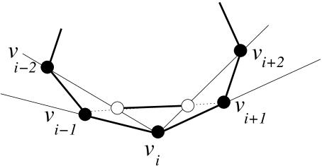
Figure 4: Points involved in the definition of the invariants

We now define a “new” invariant

$$H=\frac{1}{\prod_{i=1}^{n}z_{i}}$$ (3.19)

Remark 3.3

Some readers will know that one can put a canonical metric inside any convex shape, called the Hilbert metric. In case $\phi$ is a genuine convex polygon, the quantity $-\log(z_{k})$ measures the Hilbert length of the thick line segment in Figure 4. (The reader who does not know what the Hilbert metric is can take this as a definition.) Then $\log(H)$ is the Hilbert perimeter of $T(P)$ with respect to the Hilbert metric on $P$. Hence the name.

Lemma 3.4

$H=1/(O_{n}E_{n})$.

Proof.

This is a local calculation, which amounts to showing that $z_{k}=x_{k}y_{k}$. The best way to do the calculation is to normalize so that $4$ of the points are the vertices of a square. We omit the details. $\Box$

3.3 Compactness of the level sets

In this section, we prove that the level sets of the monodromy functions in ${\cal U\/}$ are compact.

Let ${\cal U\/}_{n}(M,H)$ denote the subset of ${\cal U\/}_{n}$ consisting of elements whose monodromy is $M$ and whose Hilbert Perimeter is $H$. In this section we will prove that ${\cal U\/}_{n}(M,H)$ is compact. For ease of notation, we abbreviate this space by $X$.

Let $\phi\in X$. We normalize so that $M$ is as in Lemma 3.1. We also normalize so that $\phi(0)=(1,1)$. Then there are numbers $(x,y)$ such that $\phi(n)=(x,y)$, independent of the choice of $\phi$. We can assume that $x>1$ and $y<1$. The portion of $\phi$ of interest to us, namely $\phi(\{0,...,n-1\})$, lies entirely in the rectangle $R$ whose two opposite corners are $(1,1)$ and $(x,y)$. Let $(v_{i},v_{j})$ denote the line determined by $v_{i}$ and $v_{j}$. Here $v_{k}=\phi(k)$. In particular, let $L_{i}=(v_{i},v_{i+1})$.

Lemma 3.5

Suppose that $\{\phi_{k}\}\in X$ is a sequence that does not converge on a subsequence to another element of $X$. Then, passing to a subsequence we can arrange that at least one of the two situations holds: there exists some $i$ such that

• The angle between $L_{i}$ and $L_{i+1}$ tends to $0$ as $k\to\infty$ whereas the angle between $L_{i+1}$ and $L_{i+2}$ does not;

• The points $v_{i}$ and $v_{i+1}$ converge to a common point as $k\to\infty$ whereas $v_{i+2}$ converges to a distinct point.

Proof.

Suppose that there is some minimum distance $\epsilon$ between all points of $\phi_{k}$ in the rectangle $R$. In this case, the angle between two consecutive segments must tend to $0$ as $k\to\infty$. However, not all angles between consecutive segments can converge to $0$ because of the fixed monodromy. The first case is now easy to arrange. If there is no such minimum $\epsilon$, then two points coalesce, on a subsequence. For the same reason as above, not all points can coalesce to the same point. The second case is now easy to arrange. $\Box$

Lemma 3.6

$X$ is compact.

We will suppose we have the kind of sequence we had in the previous lemma and then derive a contradiction. In the first case above, the slopes of the lines $(v_{i+2},v_{i})$ and $(v_{i+2},v_{i+1})$ converge to each other as $k\to\infty$, but the common limit remains uniformly bounded away from the slopes of $(v_{i+2},v_{i+3})$ and $(v_{i+2},v_{i+4})$. Hence $z_{i+2}\to 0$. Since $z_{j}\in(0,1)$ for all $j$, we have $H\to\infty$ in this case. This is a contradiction.

To deal with the second case, we can assume that the first case cannot be arranged. That is, we can assume that there is a uniform lower bound to the angles between two consecutive lines $L_{i}$ and $L_{i+1}$ for all indices and all $k$. But then the same situation as in Case 1 holds, and we get the same contradiction. $\Box$

3.4 Proof of Theorem 2

In this section, we finish the proof of Theorem 2.

Recall that the level sets of our Casimir functions give a (singular) foliation by symplectic leaves. Note that all corner invariants are nonzero for points in ${\cal U\/}_{n}$. Hence, our singular symplectic foliation intersects ${\cal U\/}_{n}$ in leaves that are all smooth symplectic manifolds. Let $k=[(n-1)/2]$.

Let $\cal M$ be a symplectic leaf. Note that $\cal M$ has dimension $4k$. Consider the map

$$F=(O_{1},E_{1},...,O_{k},E_{k}),$$ (3.20)

made from our algebraically independent monodromy invariants. Here we are excluding all the Casimirs from the definition of $F$.

Say that a point $p\in\cal M$ is regular if $dF_{p}$ is surjective. Call $\cal M$ typical if some point of $\cal M$ is regular. Given our algebraic independence result, and the fact that the coordinates of $F$ are polynomials, we see that almost every symplectic leaf is typical.

Lemma 3.7

If $\cal M$ is typical then almost every $F$-fiber of $\cal M$ is a smooth submanifold of $\cal M$.

Proof.

Let $S=F({\cal M\/})\subset{\mathbb{R}}^{2k}$. Note that $S$ has positive measure since $dF_{p}$ is nonsingular for some $p\in{\cal M\/}$. Let $\Sigma\subset\cal M$ denote the set of points $p$ such that $dF_{p}$ is not surjective. Sard’s theorem says that $F(\Sigma)$ has measure $0$. Hence, almost every fiber of $\cal M$ is disjoint from $\Sigma$. $\Box$

Let $\cal M$ be a typical symplectic leaf, and let $\cal F$ be a smooth fiber of $F$. Then $\cal F$ has dimension $2k$. Combining our Main Theorem with the standard facts about Arnold-Liouville complete integrability (e.g., [3]), we see that the monodromy invariants give a canonical affine structure to $\cal F$. The pentagram map $T$ preserves both $\cal F$, and is a translation relative to this affine structure. Any pre-compact orbit in $\cal F$ exhibits quasi-periodic motion.

Now, $T$ also preserves the monodromy. But then each $T$-orbit in $\cal F$ is contained in one of our spaces ${\cal U\/}_{n}(H,M)$. Hence, the orbit is precompact. Hence, the orbit undergoes quasi-periodic motion. Since this argument works for almost every $F$-fiber of almost every symplectic leaf in ${\cal U\/}_{n}$, we see that almost every orbit in ${\cal U\/}_{n}$ undergoes quasi-periodic motion under the pentagram map.

This completes the proof of Theorem 2.

Remark 3.8

We can say a bit more. For almost every choice of monodromy $M$, the intersection

$${\cal F\/}(M)={\cal F\/}\cap{\cal U\/}_{n}(H,M)$$ (3.21)

is a smooth compact submanifold and inherits an invariant affine structure from $\cal F$. In this situation, the restriction of $T$ to ${\cal F\/}(M)$ is a translation in the affine structure.

3.5 Hyperbolic cylinders and tight polygons

In this section, we put Theorem 2 in a somewhat broader context. The material in this section is a prelude to our proof, given in the next section, of a variant of Theorem 2.

Before we sketch variants of Theorem 2, we think about these polygons in a different way. A projective cylinder is a topological cylinder that has coordinate charts into ${\mathbb{RP}}^{2}$ such that the transition functions are restrictions of projective transformations. This is a classical example of a geometric structure. See [24] or [17] for details.

Example 3.9

Suppose that $M$ acts on ${\mathbb{R}}^{2}$ as a nontrivial diagonal matrix having eigenvalues $0<a<1<b$. Let $Q$ denote the open positive quadrant. Then $Q/M$ is a projective cylinder. We call $Q/M$ a hyperbolic cylinder.

Let $Q/M$ be a hyperbolic cylinder. Call a polygon on $Q/M$ tight if it has the following $3$ properties.

• It is embedded;

• It is locally convex;

• It is homologically nontrivial.

Any universally convex polygon gives rise to a tight polygon on $Q/M$, where $M$ is the monodromy normalized in the standard way. The converse is also true. Moreover, two tight polygons on $Q/M$ give rise to equivalent universally convex polygons iff some locally projective diffeomorphism of $Q/M$ carries one polygon to the other. We call such maps automorphisms of the cylinder, for short.

Thus, we can think of the pentagram map as giving an iteration on the space of tight polygons on a hyperbolic cylinder. There are $3$ properties that give rise to our result about periodic motion.

1. The image of a tight polygon under the pentagram map is another well-defined tight polygon.

2. The space of tight polygons on a hyperbolic cylinder, modulo the projective automorphism group, is compact.

3. The strongly diagonalizable elements are open in $SL_{3}({\mathbb{R}})$.

The third condition guarantees that the set of all tight polygons on all hyperbolic cylinders is an open subset of the set of all twisted polygons.

3.6 A related theorem

In this section we prove a variant of Theorem 2 for a different family of twisted polygons.

We start with a sector of angle $\theta$ in the plane, as shown in Figure 5, and glue the top edge to the bottom edge by a similarity $S$ that has dilation factor $d$. We omit the origin from the sector. The quotient is the projective cylinder we call $\Sigma(\theta,d)$. When $d=1$ we have a Euclidean cone surface. When $\theta=2\pi$ we have the punctured plane.

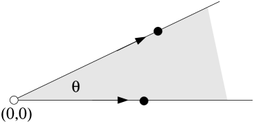
Figure 5: The cylinder $\Sigma(\theta,d)$

We consider the case when $\theta$ is small and $d$ is close to $1$. In this case, $\Sigma(\theta,d)$ admits tight polygons for any $n$. (It is easiest to think about the case when $n$ is large.) When developed out in the plane, these tight polygons follow along logarithmic spirals.

Let $S(\theta,d)$ denote the subset of ${\mathbb{R}}^{2}$ consisting of pairs $(\theta^{\prime},d^{\prime})$ where

$$0<\theta^{\prime}<\theta;\hskip 30.0pt1<d^{\prime}<d$$ (3.22)

Define

$$\widehat{\Sigma}(d,1)=\bigcup_{(\theta^{\prime},d^{\prime})\in S(\theta,d)}\Sigma(\theta^{\prime},d^{\prime})$$ (3.23)

One might say that $\widehat{\Sigma}(\theta,d)$ is the space of polygons that are more tightly coiled than those on $\Sigma(\theta,d)$.

Theorem 3

Suppose that $\theta>0$ is sufficiently close to $0$ and $d>1$ is sufficiently close to $1$. Then almost every point of $\widehat{\Sigma}(\theta,d)$ lies on a smooth torus that has a $T$-invariant affine structure. Hence, the orbit of almost every point of $\widehat{\Sigma}(\theta,d)$ undergoes quasi-periodic motion.

Proof.

Our proof amounts to verifying the three properties above for the points in our space. We fix $(\theta,d)$ and let $\widehat{\Sigma}=\widehat{\Sigma}(\theta,d)$.

1. Let $P$ be a tight polygon on $\Sigma(\theta^{\prime},d^{\prime})$. If $\theta^{\prime}$ is sufficiently small and $d^{\prime}$ is sufficiently close to $1$, then each vertex $v$ of $P$ is much closer to its neighbors than it is to the origin. For this reason, the pentagram map acts on, and preserves, the set of tight polygons on $\Sigma(\theta^{\prime},d^{\prime})$. The same goes for the inverse of the pentagram map. Hence $\widehat{\Sigma}$ is a $T$-invariant subset of ${\mathcal{P}}_{n}$.

2. Let $Z(\theta^{\prime},d^{\prime},\alpha)$ denote the space of tight polygons on $\Sigma(\theta^{\prime},d^{\prime})$ having Hilbert perimeter $\alpha$. We consider these tight polygons equivalent if there is a similarity of $\Sigma(\theta^{\prime},d^{\prime})$ that carries one to the other. A proof very much like the compactness argument given in [19], for closed polygons, shows that $Z(\theta^{\prime},d^{\prime},\alpha)$ is compact for $\theta^{\prime}$ near $0$ and $d^{\prime}$ near $1$ and $\alpha$ arbitrary. Hence, the level sets of the Casimir functions intersect $\widehat{\Sigma}$ in compact sets.

3. The similarity $S$ is the monodromy for our tight polygons. $S$ lifts to an element of $SL_{3}({\mathbb{R}})$ that has one real eigenvalue and two complex conjugate eigenvalues. Small perturbations of $S$ have the same property. Hence, $\widehat{\Sigma}$ is open in ${\mathcal{P}}_{n}$.

We have assembled all the ingredients necessary for the proof of Theorem 2. The same argument as above now establishes the result. $\Box$

Remark 3.10

The first property crucially uses the fact that $\theta$ is small. Consider the case $\theta=2\pi$. It can certainly happen that $P$ contains the origin in its hull but $T(P)$ does not. We do not know the exact bounds on $\theta$ and $d$ necessary for this construction.

4 Another coordinate system in space ${\mathcal{P}}_{n}$

4.1 Polygons and difference equations

Consider two arbitrary $n$-periodic sequences $(a_{i}),\,(b_{i})$ with $a_{i},b_{i}\in{\mathbb{R}}$ and $i\in{\mathbb{Z}}$, such that $a_{i+n}=a_{i},\,b_{i+n}=b_{i}$. Assume that $n\not=3\,m$. This will be our standing assumption whenever we work with the $(a,b)$-coordinates; its meaning will become clear shortly. We shall associate to these sequences a difference equation of the form

$$V_{i+3}=a_{i}\,V_{i+2}+b_{i}\,V_{i+1}+V_{i},$$ (4.24)

for all $i$.

A solution $V=(V_{i})$ is a sequence of numbers $V_{i}\in{\mathbb{R}}$ satisfying (4.24). Recall a well-known fact that the space of solutions of (4.24) is 3-dimensional (any solution is determined by the initial conditions $(V_{0},V_{1},V_{2})$). We will often understand $V_{i}$ as vectors in ${\mathbb{R}}^{3}$. The $n$-periodicity then implies that there exists a matrix $M\in{\mathrm{SL}}(3,{\mathbb{R}})$ called the monodromy matrix, such that $V_{i+n}=M\,V_{i}$.

Proposition 4.1

If $n$ is not divisible by 3 then the space ${\mathcal{P}}_{n}$ is isomorphic to the space of the equations (4.24).

Proof.

First note that since ${\mathrm{PGL}}(3,{\mathbb{R}})\cong{\mathrm{SL}}(3,{\mathbb{R}})$, every $M\in{\mathrm{PGL}}(3,{\mathbb{R}})$ corresponds to a unique element of ${\mathrm{SL}}(3,{\mathbb{R}})$ that (abusing the notations) we also denote by $M$.

A. Let $(v_{i}),i\in{\mathbb{Z}}$ be a sequence of points $v_{i}\in{\mathbb{RP}}^{2}$ in general position with monodromy $M$. Consider first an arbitrary lift of the points $v_{i}$ to vectors $\tilde{V}_{i}\in{\mathbb{R}}^{3}$ with the condition $\tilde{V}_{i+n}=M(\tilde{V}_{i})$. The general position property implies that $\det(\tilde{V}_{i},\tilde{V}_{i+1},\tilde{V}_{i+2})\not=0$ for all $i$. The vector $\tilde{V}_{i+3}$ is then a linear combination of the linearly independent vectors $\tilde{V}_{i+2},\tilde{V}_{i+1},\tilde{V}_{i}$, that is,

$$\tilde{V}_{i+3}=a_{i}\,\tilde{V}_{i+2}+b_{i}\,\tilde{V}_{i+1}+c_{i}\,\tilde{V}_{i},$$

for some $n$-periodic sequences $(a_{i}),\,(b_{i}),\,(c_{i})$. We wish to rescale: $V_{i}=t_{i}\tilde{V}_{i}$, so that

$$\det(V_{i},V_{i+1},V_{i+2})=1$$ (4.25)

for all $i$. Condition (4.25) is equivalent to $c_{i}\equiv 1$. One obtains the following system of equations in $(t_{1},\ldots,t_{n})$:

$$\begin{array}[]{rcll}t_{i}t_{i+1}t_{i+2}&=&1/\det(\tilde{V}_{i},\tilde{V}_{i+1},\tilde{V}_{i+2}),&i=1,\dots,n-2\\[5.0pt] t_{n-1}t_{n}t_{1}&=&1/\det(\tilde{V}_{n-1},\tilde{V}_{n},\tilde{V}_{1}),&\\[5.0pt] t_{n}t_{1}t_{2}&=&1/\det(\tilde{V}_{n},\tilde{V}_{1},\tilde{V}_{2})&\end{array}$$

This system has a unique solution if $n$ is not divisible by 3. This means that any generic twisted $n$-gon in ${\mathbb{RP}}^{2}$ has a unique lift to ${\mathbb{R}}^{3}$ satisfying (4.25). We proved that a twisted $n$-gon defines an equation (4.24) with $n$-periodic $a_{i},b_{i}$.

Furthermore, if $(v_{i})$ and $(v^{\prime}_{i}),i\in{\mathbb{Z}}$ are two projectively equivalent twisted $n$-gons, then they correspond to the same equation (4.24). Indeed, there exists $A\in{\mathrm{SL}}(3,{\mathbb{R}})$ such that $A(v_{i})=v^{\prime}_{i}$ for all $i$. One has, for the (unique) lift: $V^{\prime}_{i}=A(V_{i})$. The sequence $(V^{\prime}_{i})$ then obviously satisfies the same equation (4.24) as $(V_{i})$.

B. Conversely, let $(V_{i})$ be a sequence of vectors $V_{i}\in{\mathbb{R}}^{3}$ satisfying (4.24). Then every three consecutive points satisfy (4.25) and, in particular, are linearly independent. Therefore, the projection $(v_{i})$ to ${\mathbb{RP}}^{2}$ satisfies the general position condition. Moreover, since the sequences $(a_{i}),\,(b_{i})$ are $n$-periodic, $(v_{i})$ satisfies $v_{i+n}=M(v_{i})$. It follows that every equation (4.24) defines a generic twisted $n$-gon. A choice of initial conditions $(V_{0},V_{1},V_{2})$ fixes a twisted polygon, a different choice yields a projectively equivalent one. $\Box$

Proposition 4.1 readily implies the next result.

Corollary 4.2

If $n$ is not divisible by 3 then ${\mathcal{P}}_{n}={\mathbb{R}}^{2n}$.

We call the lift $(V_{i})$ of the sequence $(v_{i})$ satisfying equation (4.24) with $n$-periodic $(a_{i},b_{i})$ canonical.

Remark 4.3

The isomorphism between the space ${\mathcal{P}}_{n}$ and the space of difference equations (4.24) (for $n\neq 3m$) goes back to the classical ideas of projective differential geometry. This is a discrete version of the well-known isomorphism between the space of smooth non-degenerate curves in ${\mathbb{RP}}^{2}$ and the space of linear differential equations, see [17] and references therein and Section 6.1. The “arithmetic restriction” $n\not=3m$ is quite remarkable.

Equations (4.24) and their analogs were already used in [9] in the context of integrable systems; in the ${\mathbb{RP}}^{1}$-case these equations were recently considered in [14] to study the discrete versions of the Korteweg - de Vries equation. It is notable that an analogous arithmetic assumption $n\neq 2m$ is made in this paper as well.

Remark 4.4

Let us now comment on what happens if $n$ is divisible by 3. A certain modification of Proposition 4.1 holds in this case as well. Given a twisted $n$-gon $(v_{i})$ with monodromy $M$, lift points $v_{0}$ and $v_{1}$ arbitrarily as vectors $V_{0},V_{1}\in{\mathbb{R}}^{3}$, and then continue lifting consecutive points so that the determinant condition (4.25) holds. This implies that equation (4.24) holds as well.

One has:

$$M(V_{i})=t_{i}V_{i+n}$$ (4.26)

for non-zero reals $t_{i}$, and (4.25) implies that $t_{i}t_{i+1}t_{i+2}=1$ for all $i\in{\mathbb{Z}}$. It follows that the sequence $t_{i}$ is 3-periodic; let us write $t_{1+3j}=\alpha,t_{2+3j}=\beta,t_{3j}=1/(\alpha\beta)$. Applying the monodromy linear map $M$ to (4.24) and using (4.26), we conclude that

$$a_{n+i}=\frac{t_{i+2}}{t_{i}}a_{i},\ \ b_{n+i}=\frac{t_{i+1}}{t_{i}}b_{i},$$

that is,

$$\begin{split}a_{n+3j}=\alpha\beta^{2}\ a_{3j},\ a_{n+3j+1}=\frac{1}{\alpha^{2}\beta}\ a_{3j+1},\ a_{n+3j+2}=\frac{\alpha}{\beta}\ a_{3j+2},\\ b_{n+3j}=\alpha^{2}\beta\ b_{3j},\ b_{n+3j+1}=\frac{\beta}{\alpha}\ b_{3j+1},\ b_{n+3j+2}=\frac{1}{\alpha\beta^{2}}\ b_{3j+2}.\end{split}$$ (4.27)

We are still free to rescale $V_{0}$ and $V_{1}$. This defines an action of the group ${\mathbb{R}}^{*}\times{\mathbb{R}}^{*}$:

$$V_{0}\mapsto uV_{0},\ V_{1}\mapsto vV_{1},\ \ u\neq 0,v\neq 0.$$

The action of the group ${\mathbb{R}}^{*}\times{\mathbb{R}}^{*}$ on the coefficients $(a_{i},b_{i})$ is as follows:

$$\begin{split}a_{3j}\mapsto u^{2}v\ a_{3j},\ a_{3j+1}\mapsto\frac{v}{u}\ a_{3j+1},\ a_{3j+2}\mapsto\frac{1}{uv^{2}}\ a_{3j+2},\\ b_{3j}\mapsto\frac{u}{v}\ b_{3j},\ b_{3j+1}\mapsto uv^{2}\ b_{3j+1},\ b_{3j+2}\mapsto\frac{1}{u^{2}v}\ b_{3j+2}.\end{split}$$ (4.28)

When $n\neq 3m$, according to (4.27), this action makes it possible to normalize all $t_{i}$ to $1$ which makes the lift canonical. However, if $n=3m$ then the ${\mathbb{R}}^{*}\times{\mathbb{R}}^{*}$-action on $t_{i}$ is trivial, and the pair $(\alpha,\beta)\in{\mathbb{R}}^{*}\times{\mathbb{R}}^{*}$ is a projective invariant of the twisted polygon. One concludes that ${\mathcal{P}}_{n}$ is the orbit space

$$[\{(a_{0},\dots,a_{n-1},b_{0},\dots,b_{n-1})\}/({\mathbb{R}}^{*}\times{\mathbb{R}}^{*})]\times({\mathbb{R}}^{*}\times{\mathbb{R}}^{*})$$

with respect to ${\mathbb{R}}^{*}\times{\mathbb{R}}^{*}$-action (4.28). This statement replaces Proposition 4.1 in the case of $n=3m$.

It would be interesting to understand the geometric meaning of the “obstruction” $(\alpha,\beta)$. If the obstruction is trivial, that is, if $\alpha=\beta=1$, then there exists a 2-parameter family of canonical lifts, but if the obstruction is non-trivial then no canonical lift exists.

4.2 Relation between the two coordinate systems

We now have two coordinate systems, $(x_{i},y_{i})$ and $(a_{i},b_{i})$. Assuming that $n$ is not divisible by 3, let us calculate the relations between the two systems.

Lemma 4.5

One has:

$$x_{i}=\frac{a_{i-2}}{b_{i-2}\,b_{i-1}},\qquad y_{i}=-\frac{b_{i-1}}{a_{i-2}\,a_{i-1}}.$$ (4.29)

Proof.

Given four vectors $a,b,c,d$ in ${\mathbb{R}}^{3}$, the intersection line of the planes $\mathrm{Span}(a,b)$ and $\mathrm{Span}(c,d)$ is spanned by the vector $(a\times b)\times(c\times d)$. Note that the volume element equipes ${\mathbb{R}}^{3}$ with the bilinear vector product:

$${\mathbb{R}}^{3}\times{}{\mathbb{R}}^{3}\to\left({\mathbb{R}}^{3}\right)^{\star}.$$

Using the identity

$$(a\times b)\times(b\times c)=\det(a,b,c)\,b,$$ (4.30)

and the recurrence (4.24), let us compute lifts of the quadruple of points

$$\left(v_{i-1},\,v_{i},\,(v_{i-1},v_{i})\cap(v_{i+1},v_{i+2}),\,(v_{i-1},v_{i})\cap(v_{i+2},v_{i+3})\right)$$

involved in the left corner cross-ratio. One has

$$V_{i-1}=V_{i+2}-a_{i-1}\,V_{i+1}-b_{i-1}\,V_{i}.$$

Furthermore, it is easy to obtain the lift of the intersection points involved in the left corner cross-ratio. For instance, $(v_{i-1},v_{i})\cap(v_{i+1},v_{i+2})$ is

$$\begin{array}[]{rcl}\left(V_{i-1}\times{}V_{i}\right)\times\left(V_{i+1}\times{}V_{i+2}\right)&=&\left((V_{i+2}-a_{i-1}\,V_{i+1}-b_{i-1}\,V_{i})\times{}V_{i}\right)\times\left(V_{i+1}\times{}V_{i+2}\right)\\[6.0pt] &=&V_{i+2}-a_{i-1}\,V_{i+1}.\end{array}$$

One finally obtains the following four vectors in ${\mathbb{R}}^{3}$:

$$\left(V_{i+2}-a_{i-1}\,V_{i+1}-b_{i-1},V_{i},\quad V_{i},\quad V_{i+2}-a_{i-1}\,V_{i+1},\quad b_{i}\,V_{i+2}-a_{i-1}\,V_{i}-a_{i-1}\,b_{i}\,V_{i+1}\right).$$

Similarly, for the points involved in the right corner cross-ratio

$$\left(a_{i}\,V_{i+2}+b_{i},V_{i+1}+V_{i},\quad V_{i+2},\quad b_{i}\,V_{i+1}+V_{i},\quad b_{i}\,V_{i+2}-a_{i-1}\,V_{i}-a_{i-1}\,b_{i}\,V_{i+1}\right).$$

Next, given four coplanar vectors $a,b,c,d$ in ${\mathbb{R}}^{3}$ such that

$$c=\lambda_{1}\,a+\lambda_{2}\,b,\qquad d=\mu_{1}\,a+\mu_{2}\,b,$$

where $\lambda_{1},\lambda_{2},\mu_{1},\mu_{2}$ are arbitrary constants, the cross-ratio of the lines spanned by these vectors is given by

$$[a,b,c,d]=\frac{\lambda_{2}\mu_{1}-\lambda_{1}\mu_{2}}{\lambda_{2}\mu_{1}}.$$

Applying this formula to the two corner cross-ratios yields the result. $\Box$

Formula (4.29) implies the following relations:

$$x_{i}\,y_{i}=-\frac{1}{a_{i-1}\,b_{i-2}},\quad x_{i+1}\,y_{i}=-\frac{1}{a_{i-2}\,b_{i}},\quad\frac{a_{i}}{a_{i-3}}=\frac{x_{i}\,y_{i-1}}{x_{i+1}\,y_{i+1}},\quad\frac{b_{i}}{b_{i-3}}=\frac{x_{i-1}\,y_{i-1}}{x_{i+1}\,y_{i}}$$ (4.31)

that will be of use later.

Remark 4.6

If $n$ is a multiple of 3 then the coefficients $a_{i}$ and $b_{i}$ are not well defined and they are not $n$-periodic anymore; however, according to formulas (4.27) and (4.28), the right hand sides of formulas (4.29) are still well defined and are $n$-periodic.

4.3 Two versions of the projective duality

We now wish to express the pentagram map $T$ in the $(a,b)$-coordinates. We shall see that $T$ is the composition of two involutions each of which is a kind of projective duality.

The notion of projective duality in ${\mathbb{RP}}^{2}$ is based on the fact that the dual projective plane $\left({\mathbb{RP}}^{2}\right)^{\star}$ is the space of one-dimensional subspaces of ${\mathbb{RP}}^{2}$ which is again equivalent to ${\mathbb{RP}}^{2}$. Projective duality applies to smooth curves: it associates to a curve ${\gamma}(t)\subset{\mathbb{RP}}^{2}$ the 1-parameter family of its tangent lines. In the discrete case, there are different ways to define projectively dual polygons. We choose two simple versions.

Definition 4.7

Given a sequence of points $v_{i}\in{\mathbb{RP}}^{2}$, we define two sequences $\alpha(v_{i})\in({\mathbb{RP}}^{2})^{\star}$ and $\beta(v_{i})\in({\mathbb{RP}}^{2})^{\star}$ as follows:

1. $\alpha(v_{i})$ is the line $(v_{i},v_{i+1})$,

2. $\beta(v_{i})$ is the line $(v_{i-1},v_{i+1})$,

see Figure 6.

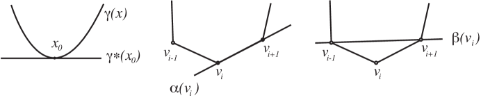
Figure 6: Projective dual for smooth curves and polygons

Clearly, $\alpha$ and $\beta$ commute with the natural ${\mathrm{PGL}}(3,{\mathbb{R}})$-action and therefore are well-defined on the space ${\mathcal{P}}_{n}$. The composition of $\alpha$ and $\beta$ is precisely the pentagram map $T$.

Lemma 4.8

One has

$$\alpha^{2}=\tau,\qquad\beta^{2}=\mathrm{Id},\qquad\alpha\circ\beta=T.$$ (4.32)

where $\tau$ is the cyclic permutation:

$$\tau(v_{i})=v_{i+1}.$$ (4.33)

Proof.

The composition of the maps $\alpha$ and $\beta$, with themselves and with each other, associates to the corresponding lines (viewed as points of $({\mathbb{RP}}^{2})^{\star}$) their intersections, see Figure 7. $\Box$

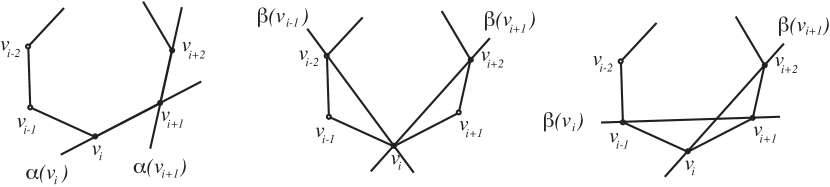
Figure 7: Iteration of the duality maps:
$\alpha^{2}(v_{i})=\alpha(v_{i})\cap\alpha(v_{i+1}),\quad\beta^{2}(v_{i})=\beta(v_{i-1})\cap\beta(v_{i+1})\quad\hbox{and}\quad(\alpha\circ\beta)(v_{i})=\beta(v_{i})\cap\beta(v_{i+1}).$

The map (4.33) defines the natural action of the group ${\mathbb{Z}}$ on ${\mathcal{P}}_{n}$. All the geometric and algebraic structures we consider are invariant with respect to this action.

4.4 Explicit formula for $\alpha$

It is easy to calculate the explicit formula of the map $\alpha$ in terms of the coordinates $(a_{i},b_{j})$. As usual, we assume $n\not=3\,m$.

Lemma 4.9

Given a twisted $n$-gon with monodromy $(v_{i}),\,i\in{\mathbb{Z}}$ represented by a difference equation (4.24), the $n$-gon $(\alpha(v_{i})),\,i\in{\mathbb{Z}}$ is represented by the equation (4.24) with coefficients

$$\alpha^{*}(a_{i})=-b_{i+1},\qquad\alpha^{*}(b_{i})=-a_{i},$$ (4.34)

where, as usual, $a^{*}$ stands for the pull-back of the coordinate functions.

Proof.

Consider the canonical lift $(V_{i})$ to ${\mathbb{R}}^{3}$. Let $U_{i}=V_{i}\times V_{i+1}\in({\mathbb{R}}^{3})^{\star}$. This is obviously a lift of the sequence $(\alpha(v_{i}))$ to $({\mathbb{R}}^{3})^{\star}$. We claim that $(U_{i})$ is, in fact, a canonical lift.

Indeed, $U_{i}$ is a lift of $u_{i}$ since $V_{i}\times V_{i+1}$ is orthogonal to $V_{i}$ and to $V_{i+1}$. Next, using the identity (4.30) one has

$$\det(U_{i}\times U_{i+1},U_{i+1}\times U_{i+2},U_{i+2}\times U_{i+3})=[(U_{i}\times U_{i+1})\times(U_{i+1}\times U_{i+2})]\cdot(U_{i+2}\times U_{i+3})$$

$$=U_{i+1}\cdot(U_{i+2}\times U_{i+3})=\det(U_{i+1},U_{i+2},U_{i+3})=1.$$

It follows that the sequence $U_{i}\in{\mathbb{R}}^{3}$ satisfies the equation

$$U_{i+3}=\alpha^{*}(a_{i})\,U_{i+2}+\alpha^{*}(b_{i})\,U_{i+1}+U_{i}$$

with some $\alpha^{*}(a_{i})$ and $\alpha^{*}(b_{i})$. Let us show that these coefficients are, indeed, given by (4.34). For all $i$, one has

$$U_{i+1}\cdot V_{i}=1,\qquad U_{i}\cdot V_{i+2}=1,\qquad U_{i+3}\cdot V_{i+3}=0.$$

Using (4.24), the last identity leads to:

$$\alpha^{*}(b_{i})\,U_{i+1}\cdot V_{i}+a_{i}\,U_{i}\cdot V_{i+2}=0.$$

Hence $\alpha^{*}(b_{i})=-a_{i}$. The first identity in (4.34) follows from formula (4.32). Indeed, one has $\alpha^{*}(\alpha^{*}(a_{i}))=a_{i+1}$ and $\alpha^{*}(\alpha^{*}(b_{i}))=b_{i+1}$, and we are done. $\Box$

4.5 Recurrent formula for $\beta$

The explicit formula for the map $\beta$ is more complicated, and we shall give a recurrent expression.

Lemma 4.10

Given an $n$-gon $(v_{i}),\,i\in{\mathbb{Z}}$ represented by a difference equation (4.24), the $n$-gon $(\beta(v_{i})),\,i\in{\mathbb{Z}}$ is represented by the equation (4.24) with coefficients

$$\beta^{*}(a_{i})=-\frac{\lambda_{i}\,b_{i-1}}{\lambda_{i+2}},\qquad\beta^{*}(b_{i})=-\frac{\lambda_{i+3}\,a_{i+1}}{\lambda_{i+1}}.$$ (4.35)

where the coefficients $\lambda_{i}$ are uniquelly defined by

$$\lambda_{i}\lambda_{i+1}\lambda_{i+2}=-\frac{1}{1+b_{i-1}a_{i}}$$ (4.36)

for all $i$.

Proof.

The lift of the map $\beta$ to ${\mathbb{R}}^{3}$ takes $V_{i}$ to $W_{i}=\lambda_{i}V_{i-1}\times V_{i+1}$ where the coefficients $\lambda_{i}$ are chosen in such a way that $\det(W_{i},W_{i+1},W_{i+2})=1$ for all $i$. The sequence $W_{i}\in{\mathbb{R}}^{3}$ satisfies the equation

$$W_{i+3}=\beta^{*}(a_{i})\,W_{i+2}+\beta^{*}(b_{i})\,W_{i+1}+W_{i}.$$

To find $\beta^{*}(a_{i})$ and $\beta^{*}(b_{i})$, one substitutes $W_{i}=\lambda_{i}V_{i-1}\times V_{i+1}$, and then, using (4.24), expresses each $V$ as a linear combination of $V_{i},V_{i+1},V_{i+2}$. The above equation is then equivalent to the following one:

$$\begin{array}[]{rcl}\left(\beta^{*}(a_{i})\,\lambda_{i+2}+b_{i-1}\,\lambda_{i}\right)V_{i}\times{}V_{i+1}&&\\[6.0pt] +\left(a_{i+1}\,\lambda_{i+3}+\beta^{*}(b_{i})\,\lambda_{i+1}\right)V_{i}\times{}V_{i+2}&&\\[6.0pt] +\left((1+b_{i}\,a_{i+1})\,\lambda_{i+3}+\beta^{*}(a_{i})\,a_{i}\,\lambda_{i+2}-\lambda_{i}\right)V_{i+1}\times{}V_{i+2}&=&0.\end{array}$$

Since the three terms are linearly independent, one obtains three relations. The first two equations lead to (4.35) while the last one gives the recurrence

$$\lambda_{i+3}=\lambda_{i}\,\frac{1+a_{i}\,b_{i-1}}{1+a_{i+1}\,b_{i}}.$$

On the other hand, one has

$$\lambda_{i}\,\lambda_{i+1}\,\lambda_{i+2}\,\det\left(V_{i-1}\times V_{i+1},V_{i}\times V_{i+2},V_{i+1}\times V_{i+3}\right)=1.$$

Once again, expressing each $V$ as a linear combination of $V_{i},V_{i+1},V_{i+2}$, yields

$$\lambda_{i}\lambda_{i+1}\lambda_{i+2}\,(1+a_{i}b_{i-1})=-1$$

and one obtains (4.36). $\Box$

4.6 Formulas for the pentagram map

We can now describe the pentagram map in terms of $(a,b)$-coordinates and to deduce formulas (2.4).

Proposition 4.11

(i) One has:

$$T^{*}(x_{i})=x_{i}\,\frac{1-x_{i-1}\,y_{i-1}}{1-x_{i+1}\,y_{i+1}},\qquad T^{*}(y_{i})=y_{i+1}\,\frac{1-x_{i+2}\,y_{i+2}}{1-x_{i}\,y_{i}}.$$

(ii) Assume that $n=3m+1$ or $n=3m+2$; in both cases,

$$T^{*}(a_{i})=a_{i+2}\,\prod_{k=1}^{m}\frac{1+a_{i+3k+2}\,b_{i+3k+1}}{1+a_{i-3k+2}\,b_{i-3k+1}},\qquad T^{*}(b_{i})=b_{i-1}\,\prod_{k=1}^{m}\frac{1+a_{i-3k-2}\,b_{i-3k-1}}{1+a_{i+3k-2}\,b_{i+3k-1}}.$$ (4.37)

Proof.

According to Lemma 4.8, $T=\alpha\circ\beta$. Combining Lemmas 4.9 and 4.10, one obtains the expression:

$$T^{*}(a_{i})=\frac{\lambda_{i+4}\,a_{i+2}}{\lambda_{i+2}},\qquad T^{*}(b_{i})=\frac{\lambda_{i}\,b_{i-1}}{\lambda_{i+2}},$$

where $\lambda_{i}$ are as in (4.36). Equation (4.29) then gives

$$\begin{array}[]{rclcl}T^{*}(x_{i})&=&\displaystyle\frac{T^{*}(a_{i-2})}{T^{*}(b_{i-2})\,T^{*}(b_{i-1})}&=&\displaystyle\frac{\lambda_{i+2}\,a_{i}}{\lambda_{i}}\,\frac{\lambda_{i}}{\lambda_{i-2}\,b_{i-3}}\,\frac{\lambda_{i+1}}{\lambda_{i-1}\,b_{i-2}}\\[16.0pt] &=&\displaystyle\frac{a_{i}}{b_{i-2}\,b_{i-3}}\,\frac{1+b_{i-3}\,a_{i-2}}{1+b_{i-1}\,a_{i}}&=&\displaystyle\frac{a_{i-3}}{b_{i-2}\,b_{i-3}}\,\frac{1+b_{i-3}\,a_{i-2}}{1+b_{i-1}\,a_{i}}\,\frac{a_{i}}{a_{i-3}}\\[16.0pt] &=&\displaystyle x_{i-1}\,\frac{1-\frac{1}{x_{i-1}\,y_{i-1}}}{1-\frac{1}{x_{i+1}\,y_{i+1}}}\,\frac{x_{i}\,y_{i-1}}{x_{i+1}\,y_{i+1}}&=&\displaystyle x_{i}\,\frac{1-x_{i-1}\,y_{i-1}}{1-x_{i+1}\,y_{i+1}},\end{array}$$

and similarly for $y_{i}$. We thus proved formula (2.4). To prove (4.37), one now uses (4.31). $\Box$

4.7 The Poisson bracket in the $(a,b)$-coordinates

The explicit formula of the Poisson bracket in the $(a,b)$-coordinates is more complicated than (2.16). Recall that $n$ is not a multiple of 3 so that we assume $n=3m+1$ or $n=3m+2$. In both cases the Poisson bracket is given by the same formula.

Proposition 4.12

The Poisson bracket (2.16) can be rewritten as follows.

$$\begin{array}[]{rcl}\{a_{i},a_{j}\}&=&\displaystyle\sum_{k=1}^{m}\left(\delta_{i,j+3k}-\delta_{i,j-3k}\right)a_{i}\,a_{j},\\[16.0pt] \{a_{i},b_{j}\}&=&0,\\[6.0pt] \{b_{i},b_{j}\}&=&\displaystyle\sum_{k=1}^{m}\left(\delta_{i,j-3k}-\delta_{i,j+3k}\right)b_{i}\,b_{j}.\end{array}$$ (4.38)

Proof.

One checks using (4.5) that the brackets between the coordinate functions $(x_{i},y_{j})$ coincide with (2.16). $\Box$

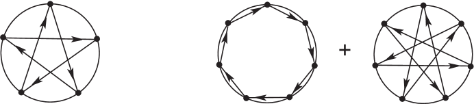
Figure 8: The Poisson bracket for $n$=5 and $n=7$.

Example 4.13

a) For $n=4$, the bracket is

$$\{a_{i},a_{j}\}=\left(\delta_{i,j+1}-\delta_{i,j-1}\right)a_{i}\,a_{j}$$

(and with opposite sign for $b$), the other terms vanish.

b) For $n=5$, the non-zero terms are:

$$\{a_{i},a_{j}\}=\left(\delta_{i,j+2}-\delta_{i,j-2}\right)a_{i}\,a_{j},$$

corresponding to the “pentagram” in Figure 8.

c) For $n=7$, one has:

$$\{a_{i},a_{j}\}=\left(\delta_{i,j+1}-\delta_{i,j-1}-\delta_{i,j+3}+\delta_{i,j-3}\right)a_{i}\,a_{j},$$

d) For $n=8$, the result is

$$\{a_{i},a_{j}\}=\left(\delta_{i,j+2}-\delta_{i,j-2}-\delta_{i,j+3}+\delta_{i,j-3}\right)a_{i}\,a_{j}.$$

5 Monodromy invariants in $(a,b)$-coordinates

The $(a,b)$-coordinates are especially well adapted to the computation of the monodromy matrix and the monodromy invariants. Such a computation provides an alternative deduction of the invariants (2.11), independent of [21].

5.1 Monodromy matrices

Consider the $3\times\infty$ matrix $M$ constructed recurrently as follows: the columns $C_{0},C_{1},C_{2},\dots$ satisfy the relation

$$C_{i+3}=a_{i}C_{i+2}+b_{i}C_{i+1}+C_{i},$$ (5.39)

and the initial $3\times 3$ matrix $(C_{0},C_{1},C_{2})$ is unit. The matrix $M$ contains the monodromy matrices of twisted $n$-gons for all $n$; namely, the following result holds.

Lemma 5.1

The $3\times 3$ minor $M_{n}=(C_{n},C_{n+1},C_{n+2})$ represents the monodromy matrix of twisted $n$-gons considered as a polynomial function in $a_{0},\dots,a_{n-1},b_{0},\dots,b_{n-1}$.

Proof.

The recurrence (5.39) coincides with (4.24), see Section 4.1. It follows that $M_{n}$ represents the monodromy of twisted $n$-gons in the basis $C_{0},C_{1},C_{2}$. $\Box$

Let

$$N_{j}=\left(\begin{array}[]{ccc}0&0&1\\ 1&0&b_{j}\\ 0&1&a_{j}\end{array}\right).$$

The recurrence (5.39) implies the following statement.

Lemma 5.2

One has: $M_{n}=N_{0}N_{1}\dots N_{n-1}$. In particular, $\det M_{n}=1$.

To illustrate, the beginning of the matrix $M$ is as follows:

$$\left(\begin{array}[]{ccccccc}1&0&0&1&a_{1}&a_{1}a_{2}+b_{2}&\dots\\ 0&1&0&b_{0}&b_{0}a_{1}+1&b_{0}a_{1}a_{2}+a_{2}+b_{0}b_{2}&\dots\\ 0&0&1&a_{0}&a_{0}a_{1}+b_{1}&a_{0}a_{1}a_{2}+b_{1}a_{2}+a_{0}b_{1}+1&\dots\end{array}\right).$$

The dihedral symmetry $\sigma$, that reverses the orientation of a polygon, replaces the monodromy matrices by their inverses and acts as follows:

$$\sigma:a_{i}\mapsto-b_{-i},\qquad b_{i}\mapsto-a_{-i};$$

this follows from rewriting equation (4.24) as

$$V_{i}=-b_{i}V_{i+1}-a_{i}V_{i+2}+V_{i+3},$$

or from Lemma 4.5.

Consider the rescaling 1-parameter group

$$\varphi_{\tau}:a_{i}\mapsto e^{\tau}a_{i},\qquad b_{i}\mapsto e^{-\tau}b_{i}.$$

It follows from Lemma 4.5 that the action on the corner invariants is as follows:

$$x_{i}\mapsto e^{3\tau}x_{i},\qquad y_{i}\mapsto e^{-3\tau}y_{i}.$$

Thus our rescaling is essentially the same as the one in (2.5) with $t=e^{3\tau}$.

The trace of $M_{n}$ is a polynomial $F_{n}(a_{0},\dots,a_{n-1},b_{0},\dots,b_{n-1})$. Denote its homogeneous components in $s:=e^{\tau}$ by $I_{j},\ j=0,\dots,[n/2]$; these are the monodromy invariants. One has $F_{n}=\sum I_{j}$. The $s$-weight of $I_{j}$ is given by the formula:

$$w(j)=3j-k\quad{\rm if}\quad n=2k,\qquad{\rm and}\quad w(j)=3j-k+1\quad{\rm if}\quad n=2k+1$$ (5.40)

(this will follow from Proposition 5.3 in the next section). For example, $M_{4}$ is the matrix

$$\left(\begin{array}[]{ccc}a_{1}&a_{1}a_{2}+b_{2}&a_{1}a_{2}a_{3}+a_{3}b_{2}+a_{1}b_{3}+1\\ a_{1}b_{0}+1&a_{1}a_{2}b_{0}+a_{2}+b_{0}b_{2}&a_{1}a_{2}a_{3}b_{0}+a_{2}a_{3}+a_{3}b_{0}b_{2}+a_{1}b_{0}b_{3}+b_{3}+b_{0}\\ a_{0}a_{1}+b_{1}&a_{0}a_{1}a_{2}+a_{2}b_{1}+a_{0}b_{2}+1&a_{0}a_{1}a_{2}a_{3}+a_{2}a_{3}b_{1}+a_{0}a_{3}b_{2}+a_{0}a_{1}b_{3}+a_{0}+a_{3}+b_{1}b_{3}\end{array}\right)$$

and

$$I_{0}=b_{0}b_{2}+b_{1}b_{3},\quad I_{1}=a_{0}+a_{1}+a_{2}+a_{3}+b_{0}a_{1}a_{2}+b_{1}a_{2}a_{3}+b_{2}a_{3}a_{0}+b_{3}a_{0}a_{1},\quad I_{2}=a_{0}a_{1}a_{2}a_{3}.$$

Likewise, for $n=5$,

$$I_{0}=\sum(b_{0}+b_{0}b_{2}a_{3}),\qquad I_{1}=\sum(a_{0}a_{1}+b_{0}a_{1}a_{2}a_{3}),\qquad I_{2}=a_{0}a_{1}a_{2}a_{3}a_{4},$$

where the sums are cyclic over the indices $0,\dots,4$.

One also has the second set of monodromy invariants $J_{0},\dots,J_{k}$ constructed from the inverse monodromy matrix, that is, applying the dihedral involution $\sigma$ to $I_{0},\dots,I_{k}$.

5.2 Combinatorics of the monodromy invariants

We now describe the polynomials $I_{i},J_{i}$ and their relation to the monodromy invariants $E_{k},O_{k}$.

Label the vertices of an oriented regular $n$-gon by $0,1,\dots,n-1$. Consider marking of the vertices by the symbols $a,b$ and $*$ subject to the rule: each marking should be coded by a cyclic word $W$ in symbols $1,2,3$ where $1=a,2=*\,b,3=***$. Call such markings admissible. If $p,q,r$ are the occurrences of $1,2,3$ in $W$ then $p+2q+3r=n$; define the weight of $W$ as $p-q$. Given a marking as above, take the product of the respective variables $a_{i}$ or $b_{i}$ that occur at vertex $i$; if a vertex is marked by $*$ then it contributes 1 to the product. Denote by $T_{j}$ the sum of these products over all markings of weight $j$. Then $A:=T_{k}$ is the product of all $a_{i}$; let $B$ be the product of all $b_{i}$; here $k=[n/2]$.

Proposition 5.3

The monodromy invariants $I_{j}$ coincide with the polynomials $T_{j}$. One has:

$$E_{j}=\frac{I_{k-j}}{A}\ {\rm for}\ j=1,\dots,k,\ {\rm and}\ E_{n}=(-1)^{n}\frac{B}{A^{2}}.$$

$J_{j}$ are described similarly by the rule $1=b,2=a\,*,3=***$, and are similarly related to $O_{j}$:

$$O_{j}=(-1)^{n+j}\frac{J_{k-j}}{B}\ {\rm for}\ j=1,\dots,k,\ {\rm and}\ O_{n}=\frac{A}{B^{2}}.$$

Proof.

First, we claim that the trace $F_{n}$ is invariant under cyclic permutations of the indices $0,1,...,n-1$.

Indeed, impose the $n$-periodicity condition: $a_{i+n}=a_{i},b_{i+n}=b_{i}$. Let $V_{i}$ be as (4.24). The matrix $M_{n}$ takes $(V_{0},V_{1},V_{2})$ to $(V_{n},V_{n+1},V_{n+2})$. Then the matrix $(V_{1},V_{2},V_{3})\to(V_{n+1},V_{n+2},V_{n+3})$ is conjugated to $M_{n}$ and hence has the same trace. This trace is $F_{n}(a_{1},b_{1},...,a_{n},b_{n})$, and due to $n$-periodicity, this equals $F_{n}(a_{1},b_{1},...,a_{0},b_{0})$. Thus $F_{n}$ is cyclically invariant.

Now we argue inductively on $n$. Assume that we know that $I_{j}=T_{j}$ for $j=n-2,n-1,n$. Consider $F_{n+1}$. Given an admissible labeling of $n-2,n-1$ or $n$-gon, one may insert $***,*\,b$ or $a$ between any two consecutive vertices, respectively, and obtain an admissible labeling of $n+1$-gon. All admissible labeling are thus obtained, possibly, in many different ways.

We claim that $F_{n+1}$ contains the cyclic sums corresponding to all admissible labeling. Indeed, consider an admissible cyclic sum in $F_{n-2}$ corresponding to a labeled $n-2$-gon $L$. This is a cyclic sum of monomials in $a_{0},...,b_{n-3}$; these monomials are located in the matrix $M$ on the diagonal of its minor $M_{n-2}$. By recurrence (5.39), the same monomials will appear on the diagonal of $M_{n+1}$, but now they must contribute to a cyclic sum of variables $a_{0},...,b_{n}$. These sums correspond to the labelings of $n+1$-gon that are obtained from $L$ by inserting $***$ between two consecutive vertices.

Likewise, consider a term in $F_{n-1}$, a cyclic sum of monomials in $a_{0},...,b_{n-2}$ corresponding to a labeled $n-1$-gon $L$. By (5.39), these monomials are to be multiplied by $b_{n-2},b_{n-1}$ or $b_{n}$ (depending on whether they appear in the first, second or third row of $M$) and moved 2 units right in the matrix $M$, after which they contribute to the cyclic sums in $F_{n+1}$. As before, the respective sums correspond to the labelings of $n+1$-gon obtained from $L$ by inserting $*\,b$ between two consecutive vertices. Similarly one deals with a contribution to $F_{n+1}$ from $F_{n}$: this time, one inserts symbol $a$.

Our next claim is that each admissible term appears in $F_{n+1}$ exactly once. Suppose not. Using cyclicity, assume this is a monomial $a_{n}P$ (or, similarly, $b_{n}P$). Where could a monomial $a_{n}P$ come from? Only from the the bottom position of the column $C_{n+2}$ (once again, according to recurrence (5.39)). But then the monomial $P$ appears at least twice in this position, hence in $F_{n}$, which contradicts our induction assumption. This completes the proof that $I_{j}=T_{j}$.

Now let us prove that $E_{j}=I_{k-j}/A$. Consider $E_{j}$ as a function of $x,y$ and switch to the $(a,b)$-coordinates using Lemma 4.5:

$$x_{1}=\frac{a_{-1}}{b_{-1}b_{0}},\qquad y_{1}=-\frac{b_{0}}{a_{-1}a_{0}}$$

and its cyclic permutations. Then

$$y_{0}x_{1}y_{1}=\frac{1}{a_{-2}a_{-1}a_{0}}$$

and the cyclic permutations. An admissible monomial in $E_{j}$ then contributes the factor $-b_{i}/(a_{i-1}a_{i})$ for each singleton $y_{i+1}$ and $1/(a_{i-2}a_{i-1}a_{i})$ for each triple $y_{i}x_{i+1}y_{i+1}$.

Admissibility implies that no index appears twice. Clear denominators by multiplying by $A$, the product of all $a$’s. Then, for each singleton $y_{i+1}$, we get the factor $-b_{i}$ and empty space $*$ at the previous position $i-1$, because there was $a_{i-1}$ in the denominator and, for each triple $y_{i}x_{i+1}y_{i+1}$, we get empty spaces $***$ at positions $i-2,i-1,i$. All other, “free”, positions are filled with $a$’s. In other words, the rule $1=a,2=*\,b,3=***$ applies. The signs are correct as well, and the result follows.

Finally, $E_{n}$ is the product of all $y_{i+1}$, that is, of the terms $-b_{i}/(a_{i-1}a_{i})$. This product equals $(-1)^{n}B/A^{2}$. $\Box$

Remark 5.4

Unlike the invariants $O_{k},E_{k}$, there are no signs involved: all the terms in polynomials $I_{i}$ are positive.

Similarly to Remark 4.6, the next lemma shows that one can use Proposition 5.3 even if $n$ is a multiple of 3. In particular, this will be useful in Theorem 4 in the next section.

Lemma 5.5

If $n$ is a multiple of 3 then the polynomials $I_{j},J_{j}$ of variables $a_{0},\dots,b_{n-1}$ are invariant under the action of the group ${\mathbb{R}}^{*}\times{\mathbb{R}}^{*}$ given in (4.28).

Proof.

Recall that, by Lemma 5.2, $M_{n}=N_{0}N_{1}\dots N_{n-1}$ where

$$N_{j}=\left(\begin{array}[]{ccc}0&0&1\\ 1&0&b_{j}\\ 0&1&a_{j}\end{array}\right).$$

The action of ${\mathbb{R}}^{*}\times{\mathbb{R}}^{*}$ on the matrices $N_{j}$ depends on $j$ mod 3 and is given by the next formulas:

$$\left(\begin{array}[]{ccc}0&0&1\\ 1&0&b_{0}\\ 0&1&a_{0}\end{array}\right)\mapsto\left(\begin{array}[]{ccc}0&0&1\\ 1&0&\frac{u}{v}\ b_{0}\\ 0&1&u^{2}v\ a_{0}\end{array}\right)=\left(\begin{array}[]{ccc}1&0&0\\ 0&\frac{u}{v}&0\\ 0&0&u^{2}v\end{array}\right)\left(\begin{array}[]{ccc}0&0&1\\ 1&0&b_{0}\\ 0&1&a_{0}\end{array}\right)\left(\begin{array}[]{ccc}\frac{v}{u}&0&0\\ 0&\frac{1}{u^{2}v}&0\\ 0&0&1\end{array}\right),$$

$$\left(\begin{array}[]{ccc}0&0&1\\ 1&0&b_{1}\\ 0&1&a_{1}\end{array}\right)\mapsto\left(\begin{array}[]{ccc}0&0&1\\ 1&0&uv^{2}\ b_{1}\\ 0&1&\frac{v}{u}\ a_{1}\end{array}\right)=\left(\begin{array}[]{ccc}1&0&0\\ 0&uv^{2}&0\\ 0&0&\frac{v}{u}\end{array}\right)\left(\begin{array}[]{ccc}0&0&1\\ 1&0&b_{1}\\ 0&1&a_{1}\end{array}\right)\left(\begin{array}[]{ccc}\frac{1}{uv^{2}}&0&0\\ 0&\frac{u}{v}&0\\ 0&0&1\end{array}\right),$$

$$\left(\begin{array}[]{ccc}0&0&1\\ 1&0&b_{2}\\ 0&1&a_{2}\end{array}\right)\mapsto\left(\begin{array}[]{ccc}0&0&1\\ 1&0&\frac{1}{u^{2}v}\ b_{2}\\ 0&1&\frac{1}{uv^{2}}\ a_{2}\end{array}\right)=\left(\begin{array}[]{ccc}1&0&0\\ 0&\frac{1}{u^{2}v}&0\\ 0&0&\frac{1}{uv^{2}}\end{array}\right)\left(\begin{array}[]{ccc}0&0&1\\ 1&0&b_{2}\\ 0&1&a_{2}\end{array}\right)\left(\begin{array}[]{ccc}u^{2}v&0&0\\ 0&uv^{2}&0\\ 0&0&1\end{array}\right).$$

Note that

$$\left(\begin{array}[]{ccc}\frac{v}{u}&0&0\\ 0&\frac{1}{u^{2}v}&0\\ 0&0&1\end{array}\right)\left(\begin{array}[]{ccc}1&0&0\\ 0&uv^{2}&0\\ 0&0&\frac{v}{u}\end{array}\right)=\frac{v}{u}\ E,\ \left(\begin{array}[]{ccc}\frac{1}{uv^{2}}&0&0\\ 0&\frac{u}{v}&0\\ 0&0&1\end{array}\right)\left(\begin{array}[]{ccc}1&0&0\\ 0&\frac{1}{u^{2}v}&0\\ 0&0&\frac{1}{uv^{2}}\end{array}\right)=\frac{1}{uv^{2}}\ E,$$

and

$$\left(\begin{array}[]{ccc}u^{2}v&0&0\\ 0&uv^{2}&0\\ 0&0&1\end{array}\right)\left(\begin{array}[]{ccc}1&0&0\\ 0&\frac{u}{v}&0\\ 0&0&u^{2}v\end{array}\right)=u^{2}v\ E,$$

where $E$ is the unit matrix. Therefore the ${\mathbb{R}}^{*}\times{\mathbb{R}}^{*}$-action on $M_{n}$ is as follows:

$$M_{n}\mapsto\frac{1}{u^{2}v}\left(\begin{array}[]{ccc}1&0&0\\ 0&\frac{u}{v}&0\\ 0&0&u^{2}v\end{array}\right)N_{0}N_{1}\dots N_{n-1}\left(\begin{array}[]{ccc}u^{2}v&0&0\\ 0&uv^{2}&0\\ 0&0&1\end{array}\right)\sim M_{n},$$

where $\sim$ means “is conjugated to”. It follows that the trace of $M_{n}$, as a polynomial in $a_{0},\dots,b_{n-1}$, is ${\mathbb{R}}^{*}\times{\mathbb{R}}^{*}$-invariant, and so are all its homogeneous components. $\Box$

5.3 Closed polygons

A closed $n$-gon (as opposed to merely twisted one) is characterized by the condition that $M_{n}=Id$. This implies that $\sum I_{j}=3$ (and, of course, $\sum J_{j}=3$ as well). There are other linear relations on the monodromy invariants which we discovered in computer experiments. All combined, we found five identities.

Theorem 4

For a closed $n$-gon, one has:

$$\sum_{j=0}^{k}I_{j}=\sum_{j=0}^{k}J_{j}=3,\quad\sum_{j=0}^{k}w(j)I_{j}=\sum_{j=0}^{k}w(j)J_{j}=0,\quad\sum_{j=0}^{k}w(j)^{2}(I_{j}-J_{j})=0,$$

where $k=[n/2]$ and $w(j)$ are the weights (5.40).

Proof.

The monodromy $M\in SL(3,{\mathbb{R}})$ is a matrix-valued polynomial function of $a_{i},b_{i}$, and $M(\tau)=M\circ\varphi_{\tau}$ where $\varphi_{\tau}$ is the scaling action

$$a_{i}\mapsto e^{\tau}a_{i},\quad b_{i}\mapsto e^{-\tau}b_{i}.$$

The characterization of ${\cal C}_{n}$ is $M(0)=Id$.

Let $e^{\lambda_{1}},e^{\lambda_{2}},e^{\lambda_{3}}$ be the eigenvalues of $M(\tau)$ considered as functions of $a_{i},b_{i},\tau$. Then $\lambda_{i}=0$ for $\tau=0$ and each $i=1,2,3$, and

$$\lambda_{1}+\lambda_{2}+\lambda_{3}=0$$ (5.41)

identically. The eigenvalues of $M^{-1}$ are similar with negative $\lambda$s as exponents. The definition of $I(a,b)$ and $J(a,b)$ implies:

$$e^{\lambda_{1}}+e^{\lambda_{2}}+e^{\lambda_{3}}=\sum e^{\tau w(j)}I_{j},\ e^{-\lambda_{1}}+e^{-\lambda_{2}}+e^{-\lambda_{3}}=\sum e^{-\tau w(j)}J_{j},$$ (5.42)

where $w(j)$ are the weights. Setting $\tau=0$ in (5.42) we obtain the obvious relations $\sum I_{j}=\sum J_{j}=3$. Differentiating (5.42) with respect to $\tau$ and setting $\tau=0$, we get

$$\sum_{i=1}^{3}\lambda_{i}^{\prime}(0)=\sum w(j)I_{j}=\sum w(j)J_{j}.$$

By (5.41), the left hand side is zero, and we obtain two other relations stated in the theorem.

Differentiate (5.42) twice and set $\tau=0$:

$$\sum_{i=1}^{3}\lambda_{i}^{\prime\prime}(0)+\lambda_{i}^{\prime}(0)^{2}=\sum w(j)^{2}I_{j},\ \sum_{i=1}^{3}-\lambda_{i}^{\prime\prime}(0)+\lambda_{i}^{\prime}(0)^{2}=\sum w(j)^{2}J_{j}.$$

Subtract and use the fact that $\sum_{i=1}^{3}\lambda_{i}^{\prime\prime}(0)=0$ (as follows from (5.41) by differentiating in $\tau$ twice) to obtain:

$$\sum w(j)^{2}(I_{j}-J_{j})=0.$$ (5.43)

This is the fifth relation of the theorem. $\Box$

Example 5.6

In the cases $n=4$ and $n=5$, it is easy to solve the equation $M_{n}=Id$. For $n=4$, the solution is a single point

$$a_{0}=a_{1}=a_{2}=a_{3}=1,\qquad b_{0}=b_{1}=b_{2}=b_{3}=-1,$$

and then $I_{0}=2,I_{1}=0,I_{2}=1$. For $n=5$, one has a 2-parameter set of solutions with free parameters $x,y$:

$$a_{0}=x,\quad a_{1}=y,\quad a_{2}=-\frac{1+x}{1-xy},\quad a_{3}=-(1-xy),\quad a_{4}=-\frac{1+y}{1-xy},$$

and $b_{i}=-a_{i+2}$. Hence

$$I_{0}=J_{0}=2-z,\ I_{1}=J_{1}=1+2z,\ I_{2}=J_{2}=-z\ \ {\rm with}\ \ z=\frac{xy(1+x)(1+y)}{1-xy}.$$

Remark 5.7

${\cal C\/}_{n}$ has codimension 8 in ${\cal P\/}_{n}$, and we have the five relations of Theorem 4. We conjecture that there are no other relations between the monodromy invariants that hold identically on ${\cal C}_{n}$.

6 Continuous limit: the Boussinesq equation

Since the theory of infinite-dimensional integrable systems on functional spaces is much more developed than the theory of discrete integrable systems, it is important to investigate the $n\to\infty$ “continuous limit” of the pentagram map.

It turns out that the continuous limit of $T$ is the classical Boussinesq equation. This is quite remarkable since the Boussinesq equation and its discrete analogs are thoroughly studied but, to the best of our knowledge, their geometrical interpretation remained unknown.

We will also show that the Poisson bracket (2.16) can be viewed as a discrete version of the well-known first Poisson structure of the Boussinesq equation.

6.1 Non-degenerate curves and differential operators

We understand the continuous limit of a twisted $n$-gon as a smooth parametrized curve ${\gamma}:{\mathbb{R}}\to{\mathbb{RP}}^{2}$ with monodromy:

$${\gamma}(x+1)=M({\gamma}(x)),$$ (6.44)

for all $x\in{\mathbb{R}}$, where $M\in PSL(3,{\mathbb{R}})$ is fixed. The assumption that every three consequtive points are in general position corresponds to the assumption that the vectors ${\gamma}^{\prime}(x)$ and ${\gamma}^{\prime\prime}(x)$ are linearly independent for all $x\in{\mathbb{R}}$. A curve ${\gamma}$ satisfying these conditions is usually called non-degenerate.

As in the discrete case, we consider classes of projectively equivalent curves. The continuous analog of the space ${\cal P}_{n}$, is then the space, ${\cal C}$, of parametrized non-degenerate curves in ${\mathbb{RP}}^{2}$ up to projective transformations. The space ${\cal C}$ is very well known in classical projective differential geometry, see, e.g., [17] and references therein.

Proposition 6.1

There exists a one-to-one correspondence between ${\cal C}$ and the space of linear differential operators on ${\mathbb{R}}$:

$$A=\left(\frac{d}{dx}\right)^{3}+u(x)\,\frac{d}{dx}+v(x),$$ (6.45)

where $u$ and $v$ are smooth periodic functions.

This statement is classical, but we give here a sketch of the proof.

Proof.

A non-degenerate curve ${\gamma}(x)$ in ${\mathbb{RP}}^{2}$ has a unique lift to ${\mathbb{R}}^{3}$, that we denote by ${\Gamma}(x)$, satisfying the condition that the determinant of the vectors ${\Gamma}(x),{\Gamma}^{\prime}(x),{\Gamma}^{\prime\prime}(x)$ (the Wronskian) equals 1 for every $x$:

$$\left|{\Gamma}(x)\,{\Gamma}^{\prime}(x)\,{\Gamma}^{\prime\prime}(x)\right|=1.$$ (6.46)

The vector ${\Gamma}^{\prime\prime\prime}(x)$ is a linear combination of ${\Gamma}(x),{\Gamma}^{\prime}(x),{\Gamma}^{\prime\prime}(x)$ and the condition (6.46) is equivalent to the fact that this combination does not depend on ${\Gamma}^{\prime\prime}(x)$. One then obtains:

$${\Gamma}^{\prime\prime\prime}(x)+u(x)\,{\Gamma}^{\prime}(x)+v(x)\,{\Gamma}(x)=0.$$

Two curves in ${\mathbb{RP}}^{2}$ correspond to the same operator if and only if they are projectively equivalent.

Conversely, every differential operator (6.45) defines a curve in ${\mathbb{RP}}^{2}$. Indeed, the space of solutions of the differential equation $A\,f=0$ is 3-dimensional. At any point $x\in{\mathbb{R}}$, one considers the 2-dimensional subspace of solutions vanishing at $x$. This defines a curve in the projectivization of the space dual to the space of solutions. $\Box$

Remark 6.2

It will be convenient to rewrite the above differential operator as a sum of a skew-symmetric operator and a (zero-order) symmetric operator:

$$A=\left(\frac{d}{dx}\right)^{3}+\frac{1}{2}\left(u(x)\,\frac{d}{dx}+\frac{d}{dx}\,u(x)\right)+w(x)$$ (6.47)

where $w(x)=v(x)-\frac{u^{\prime}(x)}{2}$. The pair of functions $(u,w)$ is understood as the continuous analog of the coordinates $(a_{i},b_{i})$.

6.2 Continuous limit of the pentagram map

We are now defining a continuous analog of the map $T$. The construction is as follows. Given a non-degenerate curve ${\gamma}(x)$, at each point $x$ we draw a small chord: $\left({\gamma}(x-{\varepsilon}),{\gamma}(x+{\varepsilon})\right)$ and obtain a new curve, ${\gamma}_{\varepsilon}(x)$, as the envelop of these chords, see Figure 9.

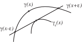
Figure 9: Evolution of a non-degenerate curve

The differential operator (6.47) corresponding to ${\gamma}_{\varepsilon}(x)$ contains new functions $(u_{\varepsilon},w_{\varepsilon})$. We will show that

$$u_{\varepsilon}=u+{\varepsilon}^{2}\widetilde{u}+O({\varepsilon}^{3}),\qquad w_{\varepsilon}=w+{\varepsilon}^{2}\widetilde{w}+O({\varepsilon}^{3})$$

and calculate $\widetilde{u},\widetilde{w}$ explicitly. We then assume that the functions $u(x)$ and $w(x)$ depend on an additional parameter $t$ (the “time”) and define an evolution equation:

$$\dot{u}=\widetilde{u},\qquad\dot{w}=\widetilde{w}$$

that we undestand as a vector field on the space of functions (and therefore of operators (6.47)). Here and below $\dot{u}$ and $\dot{w}$ are the partial derivatives in $t$, the partial derivatives in $x$ will be denoted by ^′.

Theorem 5

The continuous limit of the pentagram map $T$ is the following equation:

$$\begin{array}[]{rcl}\displaystyle\dot{u}&=&w^{\prime},\\[10.0pt] \displaystyle\dot{w}&=&\displaystyle-\frac{u\,u^{\prime}}{3}-\frac{u^{\prime\prime\prime}}{12},\end{array}$$ (6.48)

Proof.

The (lifted) curve ${\Gamma}_{\varepsilon}\subset{\mathbb{R}}^{3}$, corresponding to ${\gamma}_{\varepsilon}(x)$ satisfies the following conditions:

$$\begin{array}[]{rcl}\left|{\Gamma}(x+{\varepsilon}),\,{\Gamma}(x-{\varepsilon}),\,{\Gamma}_{\varepsilon}(x)\right|&=&0,\\[6.0pt] \left|{\Gamma}_{\varepsilon}(x),\,{\Gamma}(x+{\varepsilon})-{\Gamma}(x-{\varepsilon}),\,{\Gamma}_{\varepsilon}^{\prime}(x)\right|&=&0.\end{array}$$

We assume that the curve ${\Gamma}_{\varepsilon}(x)$ is of the form:

$${\Gamma}_{\varepsilon}={\gamma}+{\varepsilon}\,A+{\varepsilon}^{2}\,B+({\varepsilon}^{3}),$$

where $A$ and $B$ are some vector-valued functions. The above conditions easily imply that $A$ is proportional to ${\Gamma}$, while $B$ satisfies:

$$\begin{array}[]{rcl}\left|{\Gamma}(x),\,{\Gamma}^{\prime}(x),\,B^{\prime}(x)\right|&=&0,\\[6.0pt] \frac{1}{2}\left|{\Gamma}(x),\,{\Gamma}^{\prime}(x),\,{\Gamma}^{\prime\prime}(x)\right|+\left|{\Gamma}(x),\,{\Gamma}^{\prime}(x),\,B(x)\right|&=&0.\end{array}$$

It follows that $B=\frac{1}{2}{\Gamma}^{\prime\prime}+g{\Gamma}$, where $g$ is a function. We proved that the curve ${\Gamma}_{\varepsilon}(x)$ is of the form:

$$\textstyle{\Gamma}_{\varepsilon}=\left(1+{\varepsilon}{}f+{\varepsilon}^{2}g\right){\Gamma}+\frac{{\varepsilon}^{2}}{2}\,{\Gamma}^{\prime\prime}+({\varepsilon}^{3}),$$

where $f$ and $g$ are some functions.

It remains to find $f$ and $g$ and the corresponding differential operator. To this end one has to use the normalization condition (6.46).

Lemma 6.3

The condition (6.46) implies $f(x)\equiv 0$ and $g(x)=\frac{u(x)}{3}$.

Proof.

A straightforward computation. $\Box$

One has finally the following expression for the lifted curve:

$${\Gamma}_{\varepsilon}=\left(1+\frac{{\varepsilon}^{2}}{3}u\right){\Gamma}+\frac{{\varepsilon}^{2}}{2}\,{\Gamma}^{\prime\prime}+({\varepsilon}^{3}).$$ (6.49)

We are ready to find the new functions $u_{\varepsilon},v_{\varepsilon}$ such that

$${\Gamma}_{\varepsilon}^{\prime\prime\prime}(x)+u_{\varepsilon}(x)\,{\Gamma}_{\varepsilon}^{\prime}(x)+v_{\varepsilon}(x)\,{\Gamma}_{\varepsilon}(x)=0.$$

After a straighforward calculation, using the additional formula

$${\Gamma}^{(V)}=-(2u^{\prime}+v)\,{\Gamma}^{\prime\prime}-(u^{\prime\prime}+2v^{\prime}-u^{2})\,{\Gamma}^{\prime}-(v^{\prime\prime}-uv)\,{\Gamma},$$

one gets directly from (6.49):

$$u_{\varepsilon}=u+{\varepsilon}^{2}\left(v^{\prime}-\frac{u^{\prime\prime}}{2}\right),\qquad v_{\varepsilon}=v+{\varepsilon}^{2}\left(\frac{v^{\prime\prime}}{2}-\frac{uu^{\prime}}{3}-\frac{u^{\prime\prime\prime}}{3}\right).$$

The result follows. $\Box$

Remark 6.4

Equation (6.48) is equivalent to the following differential equation

$$\ddot{u}=-\frac{\left(u^{2}\right)^{\prime\prime}}{6}-\frac{u^{(IV)}}{12},$$

which is nothing else but the classical Boussinesq equation.

Remark 6.5

It is not hard to compute that the continuous limit of the scaling symmetry is given by the formula:

$$u(x)\mapsto u(x),\quad w(x)\mapsto w(x)+t$$

where $t$ is a constant.

Remark 6.6

The fact that the continuous limit of the pentagram map is the Boussinesq equation is discovered in [19] (not much details are provided). The computation in [19] is made in an affine chart ${\mathbb{R}}^{2}\subset{\mathbb{RP}}^{2}$. In this lift, different from the canonical one (characterized by constant Wronskian), one obtains the curve flow

$${\dot{\Gamma}}=-\frac{1}{3}\frac{[{\Gamma}^{\prime},{\Gamma}^{\prime\prime\prime}]}{[{\Gamma}^{\prime},{\Gamma}^{\prime\prime}]}{\Gamma}^{\prime}+\frac{1}{2}{\Gamma}^{\prime\prime}$$

where $[.,.]$ is the cross-product; this is equivalent to equation (6.49) (we omit a rather tedious verification of this equivalence).

6.3 The constant Poisson structure

The equation (6.48) is integrable. In particular, it is Hamiltonian with respect to (two) Poisson structures on the space of functions $(u,w)$. We describe here the simplest Poisson structure usually called the first Poisson structure of the Boussinesq equation.

Consider the space of functionals of the form

$$H(u,w)=\int_{S^{1}}h(u,u^{\prime},\ldots,w,w^{\prime},\ldots)\,dx,$$

where $h$ is a polynomial. The variational derivatives, $\delta_{u}H$ and $\delta_{w}H$, are the smooth functions on $S^{1}$ given by the Euler-Lagrange formula, e.g.,

$$\delta_{u}H=\frac{\partial{}h}{\partial{}u}-\left(\frac{\partial{}h}{\partial{}u^{\prime}}\right)^{\prime}+\left(\frac{\partial{}h}{\partial{}u^{\prime\prime}}\right)^{\prime\prime}-+\cdots$$

and similarly for $\delta_{w}H$.

Definition 6.7

The constant Poisson structure on the space of functionals is defined by

$$\{G,H\}=\int_{S^{1}}\left(\delta_{u}G\left(\delta_{w}H\right)^{\prime}+\delta_{w}G\left(\delta_{u}H\right)^{\prime}\right)dx.$$ (6.50)

Note that the “functional coordinates” $\left(u(x),w(x)\right)$ play the role of Darboux coordinates.

Another way to define the above Poisson structure is as follows. Given a functional $H$ as above, the Hamiltonian vector field with Hamiltonian $H$ is given by

$$\begin{array}[]{rcl}\displaystyle\dot{u}&=&\left(\delta_{w}H\right)^{\prime},\\[6.0pt] \displaystyle\dot{w}&=&\displaystyle\left(\delta_{u}H\right)^{\prime}.\end{array}$$ (6.51)

The following statement is well known, see, e.g., [8].

Proposition 6.8

The function

$$H=\int_{S^{1}}\left(\frac{w^{2}}{2}-\frac{u^{3}}{18}-\frac{uu^{\prime\prime}}{24}\right)dx$$

is the Hamiltonian function for the equation (6.48).

Proof.

Straighforward from (6.51). $\Box$

This statement has many consequences. For instance, the following functions are the first integrals of (6.48):

$$H_{1}=\int_{S^{1}}u\,dx,\qquad H_{2}=\int_{S^{1}}w\,dx,\qquad H_{3}=\int_{S^{1}}uw\,dx.$$

Note that the functions $H_{1}$ and $H_{2}$ are precisely the Casimir functions of the structure (6.51).

6.4 Discretization

Let us now test the inverse procedure of discretization. Being more “heuristic”, this procedure will nevertheless be helpful for understanding the discrete limit of the classical Poisson structure of the Boussinesq equation.

Given a non-degenerate curve ${\gamma}(x)$, fix an arbitrary point $v_{i}:={\gamma}(x)$ and, for a small ${\varepsilon}$, set $v_{i+1}:={\gamma}(x+{\varepsilon})$, etc. We then have:

$$v_{i}={\gamma}(x),\qquad v_{i+1}={\gamma}(x+{\varepsilon})\qquad v_{i+2}={\gamma}(x+2\,{\varepsilon})\qquad v_{i+3}={\gamma}(x+3\,{\varepsilon}).$$

Lifting ${\gamma}(x)$ and $(v_{i})$ to ${\mathbb{R}}^{3}$ so that the difference equation (4.24) be satisfied, we are looking for $a$ and $b$ in

$${\Gamma}(x+3\,{\varepsilon})=a(x,{\varepsilon})\,{\Gamma}(x+2\,{\varepsilon})+b(x,{\varepsilon})\,{\Gamma}(x+{\varepsilon})+{\Gamma}(x),$$

as functions of $x$ depending on ${\varepsilon}$, where ${\varepsilon}$ is small.

Lemma 6.9

Representing $a(x)$ and $b(x)$ as a series in ${\varepsilon}$:

$$a(x,{\varepsilon})=a_{0}(x)+{\varepsilon}\,a_{1}(x)+\cdots,\qquad b(x,{\varepsilon})=b_{0}(x)+{\varepsilon}\,b_{1}(x)+\cdots,$$

one gets for the first four terms:

$$\begin{array}[]{ll}a_{0}=3,&b_{0}=-3,\\[4.0pt] a_{1}=0,&b_{1}=0,\\[4.0pt] a_{2}=-u(x),&b_{2}=u(x),\\[6.0pt] a_{3}=-\frac{7}{4}\,u^{\prime}(x)-\frac{1}{2}\,w(x),&b_{3}=\frac{5}{4}\,u^{\prime}(x)-\frac{1}{2}\,w(x).\end{array}$$ (6.52)

Proof.

Straighforward Taylor expansion of the above expression for ${\Gamma}(x+3\,{\varepsilon})$. $\Box$

The Poisson structure (2.16) can be viwed as a discrete analog of the structure (6.50) and this is, in fact, the way we guessed it. Indeed, one has the following two observations.

(1) Formula (6.52) shows that the functions $\log{a}$ and $\log{b}$ are approximated by linear combinations of $u$ and $w$ and therefore (4.38), a discrete analog of the bracket (6.50), should be a constant bracket in the coordinates $(\log{a},\log{b})$.

(2) Consider the following functionals (linear in the $(a,b)$-coordinates):

$$F_{f}(a,b)=\int_{S^{1}}f(x)\,a(x,{\varepsilon})\,dx,\qquad G_{f}(a,b)=\int_{S^{1}}f(x)\,b(x,{\varepsilon})\,dx.$$

Using (6.50) and (6.52), one obtains:

$$\{F_{f},\,F_{g}\}={\varepsilon}^{5}\int_{S^{1}}fg^{\prime}\,dx+O({\varepsilon}^{6}),\quad\{F_{f},\,G_{g}\}=O({\varepsilon}^{6}),\quad\{G_{f},\,G_{g}\}=-{\varepsilon}^{5}\int_{S^{1}}fg^{\prime}\,dx+O({\varepsilon}^{6}).$$

One immediately derives the following general form of the “discretized” Poisson bracket on the space ${\mathcal{P}}_{n}$:

$$\{a_{i},a_{j}\}=P_{i,j}\,a_{i}a_{j},\qquad\{a_{i},b_{j}\}=0,\qquad\{b_{i},b_{j}\}=-P_{i,j}\,b_{i}b_{j},$$

where $P_{i,j}$ are some constants. Furthermore, one assumes: $P_{i+k,j+k}=P_{i,j}$ by cyclic invariance. One then can check that (4.38) is the only Poisson bracket of the above form preserved by the map $T$.

7 Discussion

We finish this paper with questions and conjectures.

Second Poisson structure.

The Poisson structure (2.16) is a discretization of (6.50) known as the first Poisson structure of the Boussinesq equation. We believe that there exists another, second Poisson structure, compatible with the Poisson structure (2.16), that allows to obtain the monodromy invariants (and thus to prove integrability of $T$) via the standard bi-Hamiltonian procedure.

Note that the Poisson structure usually considered in the discrete case, cf. [9], is a discrete version of the second Adler-Gelfand-Dickey bracket. We conjecture that one can adapt this bracket to the case of the pentagram map.

Integrable systems on cluster manifolds.

The space ${\mathcal{P}}_{n}$ is closely related to cluster manifolds, cf. [7]. The Poisson bracket (2.16) is also similar to the canonical Poisson bracket on a cluster manifold, cf. [10].

Example 5.6 provides a relation of the $(a,b)$-coordinates to the cluster coordinates. A twisted pentagon is closed if and only if

$$a_{0}=\frac{a_{3}+1}{a_{1}},\qquad a_{2}=\frac{a_{1}+a_{3}+1}{a_{1}\,a_{3}},\qquad a_{4}=\frac{a_{1}+1}{a_{3}},$$

and $b_{i}=-a_{i+2}$. Note that $a_{i+5}=a_{i}$. This formula coincides with formula of coordinate exchanges for the cluster manifold of type $A_{2}$, see [7]. The 2-dimensional submanifold of ${\mathcal{P}}_{5}$ with $M=\mathrm{Id}$ is therefore a cluster manifold; the coordinates $(a_{1},a_{3})$, etc. are the cluster variables.

It would be interesting to compare the coordinate systems on ${\mathcal{P}}_{n}$ naturally arising from our projective geometrical approach with the canonical cluster coordinates and check whether the Poisson bracket constructed in this paper coincides with the canonical cluster Poisson bracket.

We think that analogs of the pentagram map may exist for a larger class of cluster manifolds.

Polygons inscribed into conics.

We observed in computer experiments that if a twisted polygon is inscribed into a conic then one has: $E_{k}=O_{k}$ for all $k$; the same holds for polygons circumscribed about conics. As of now, this is an open conjecture. Working on this conjecture, we discovered, by computer experiments, a variety of new configuration theorems of projective geometry involving polygons inscribed into conics; these results will be published separately. Let us also mention that twisted $n$-gons inscribed into a conic constitute a coisotropic submanifold of the Poisson manifold ${\cal P}_{n}$. Dynamical consequences of this observations will be studied elsewhere.

Acknowledgments. We are endebted to A. Bobenko, V. Fock, I. Marshall, S. Parmentier, M. Semenov-Tian-Shanski and Yu. Suris for stimulating discussions. V. O. and S. T. are grateful to the Research in Teams program at BIRS. S. T. is also grateful to Max-Planck-Institut in Bonn for its hospitality. R. S. and S. T. were partially supported by NSF grants, DMS-0604426 and DMS-0555803, respectively.

Valentin Ovsienko: CNRS, Institut Camille Jordan, Université Lyon 1, Villeurbanne Cedex 69622, France, ovsienko@math.univ-lyon1.fr

Serge Tabachnikov: Pennsylvania State University, Department of Mathematics University Park, PA 16802, USA, tabachni@math.psu.edu

Richard Evan Schwartz: Department of Mathematics, Brown University, Providence, RI 02912, USA, res@math.brown.edu

References

• [1] V. E. Adler, Cuttings of polygons, Funct. Anal. Appl. 27 (1993), 141–143.
• [2] V. E. Adler, Integrable deformations of a polygon, Phys. D 87 (1995), 52–57.
• [3] V.I. Arnold, Mathematical methods of classical mechanics, Graduate Texts in Mathematics, 60. Springer-Verlag, New York, 1989.
• [4] A. Belov, K. Chaltikian, Lattice analogues of $W$-algebras and classical integrable equations, Phys. Lett. B 309 (1993), 268–274.
• [5] A. Bobenko, Yu. Suris, Discrete Differential Geometry: Integrable Structure, AMS, 2008.
• [6] V. Fock, A. Goncharov, Moduli spaces of convex projective structures on surfaces, Adv. Math. 208 (2007), 249–273.
• [7] S. Fomin, A, Zelevinsky, Cluster Algebras I: Foundations, J. Amer. Math. Soc. 12 (2002), 497–529.
• [8] G. Falqui, F. Magri, G. Tondo, Reduction of bi-Hamiltonian systems and the separation of variables: an example from the Boussinesq hierarchy. Theoret. and Math. Phys. 122 (2000), 176–192.
• [9] E. Frenkel, N. Reshetikhin, M. Semenov-Tian-Shansky, Drinfeld-Sokolov reduction for difference operators and deformations of $W$-algebras. I. The case of Virasoro algebra, Comm. Math. Phys. 192 (1998), 605–629.
• [10] M. Gekhtman, M. Shapiro, A. Vainshtein, Cluster algebras and Poisson geometry, Mosc. Math. J. 3 (2003), 899–934.
• [11] A. Henriques. A periodicity theorem for the octahedron recurrence, J. Algebraic Combin. 26 (2007), 1–26.
• [12] T. Hoffmann, N. Kutz. Discrete curves in CP1 and the Toda lattice, Stud. Appl. Math. 113 (2004), 31-55.
• [13] B. G. Konopelchenko, W. K. Schief, Menelaus’ theorem, Clifford configurations and inversive geometry of the Schwarzian KP hierarchy, J. Phys. A: Math. Gen. 35 (2002), 6125–6144.
• [14] I. Marshall, M. Semenov-Tian-Shansky, Poisson groups and differential Galois theory of Schroedinger Equation on the circle, Comm. Math. Phys, 284 (2008), 537–552.
• [15] Th. Motzkin, The pentagon in the projective plane, with a comment on Napier s rule, Bull. Amer. Math. Soc. 52 (1945), 985 989.
• [16] V. Ovsienko, R. Schwartz, S. Tabachnikov, Quasiperiodic motion for the pentagram map, Electron. Res. Announc. Math. Sci. 16 (2009), 1–8.
• [17] V. Ovsienko, S. Tabachnikov, Projective differential geometry old and new, from Schwarzian derivative to the cohomology of diffeomorphism groups, Cambridge Tracts in Mathematics, 165, Cambridge University Press, Cambridge, 2005.
• [18] D. Robbins, H. Rumsey. Determinants and alternating sign matrices, Adv. Math. 62 (1986), 169–184.
• [19] R. Schwartz, The pentagram map, Experiment. Math. 1 (1992), 71–81.
• [20] R. Schwartz, The pentagram map is recurrent, Experiment. Math. 10 (2001), 519–528.
• [21] R. Schwartz, Discrete monodromy, pentagrams, and the method of condensation, J. of Fixed Point Theory and Appl. 3 (2008), 379–409.
• [22] D. Speyer. Perfect matchings and the octahedron recurrence, J. Algebraic Combin. 25 (2007), 309–348.
• [23] Yu. Suris. The problem of integrable discretization: Hamiltonian approach, Progress in Mathematics, 219, Birkhauser Verlag, Basel, 2003.
• [24] W. Thurston, Three-dimensional geometry and topology. Vol. 1, Princeton Mathematical Series, 35, Princeton University Press, Princeton, NJ, 1997.
• [25] A. Tongas, F. Nijhoff, The Boussinesq integrable system: compatible lattice and continuum structures, Glasg. Math. J. 47 (2005), 205–219.
• [26] A. Veselov, Integrable mappings, Russian Math. Surv. 46 (1991), no. 5, 1–51.
• [27] A. Weinstein, The local structure of Poisson manifolds, J. Diff. Geom. 18 (1983), 523–557.