Chemical Diversity in High-Mass Star Formation

Abstract

Massive star formation exhibits an extremely rich chemistry. However, not much evolutionary details are known yet, especially at high spatial resolution. Therefore, we synthesize previously published Submillimeter Array high-spatial-resolution spectral line observations toward four regions of high-mass star formation that are in various evolutionary stages with a range of luminosities. Estimating column densities and comparing the spatially resolved molecular emission allows us to characterize the chemical evolution in more detail. Furthermore, we model the chemical evolution of massive warm molecular cores to be directly compared with the data. The four regions reveal many different characteristics. While some of them, e.g., the detection rate of CH₃OH, can be explained by variations of the average gas temperatures, other features are attributed to chemical effects. For example, C³⁴S is observed mainly at the core-edges and not toward their centers because of temperature-selective desorption and successive gas-phase chemistry reactions. Most nitrogen-bearing molecules are only found toward the hot molecular cores and not the earlier evolutionary stages, indicating that the formation and excitation of such complex nitrogen-bearing molecules needs significant heating and time to be fully developed. Furthermore, we discuss the observational difficulties to study massive accretion disks in the young deeply embedded phase of massive star formation. The general potential and limitations of such kind of dataset are discussed, and future directions are outlined. The analysis and modeling of this source sample reveals many interesting features toward a chemical evolutionary sequence. However, it is only an early step, and many observational and theoretical challenges in that field lie ahead.

1. Introduction

One of the main interests in high-mass star formation research today is a thorough characterization of the expected massive accretion disks (e.g., Yorke & Sonnhalter 2002; Krumholz et al. 2007). Observations of this type require high spatial resolution, and disks have been suggested in numerous systems, although not always with the same tracers (for a recent compilation see Cesaroni et al. 2007). A major complication is the large degree of chemical diversity in these regions.  This is seen on large scales in terms of the large number of molecular detections (e.g., Schilke et al. 1997; van Dishoeck & Blake 1998) but in particular on the small scale (of the order $10^{4}$ AU and even smaller) where significant chemical differentiation is found (e.g., Beuther et al. 2005a).   At present, we are only beginning to decipher the chemical structure of these objects at high spatial resolution, whereas our understanding of the physical properties better allows us to place regions into an evolutionary context (e.g., Beuther et al. 2007a; Zinnecker & Yorke 2007). It is not yet clear how our emerging picture of the physical evolution is related to the observed chemical diversity and evolution.

Various theory groups work on the chemical evolution during massive star formation (e.g., Caselli et al. 1993; Millar et al. 1997; Charnley 1997; Viti et al. 2004; Nomura & Millar 2004; Wakelam et al. 2005; Doty et al. 2002, 2006), and the results are promising. However, the observational database to test these models against is still relatively poor. Some single-dish low-spatial-resolution line surveys toward several sources do exist, but they are all conducted with different spatial resolution and covering different frequency bands (e.g., Blake et al. 1987; MacDonald et al. 1996; Schilke et al. 1997; Hatchell et al. 1998; McCutcheon et al. 2000; van der Tak et al. 2000, 2003; Johnstone et al. 2003; Bisschop et al. 2007). Furthermore, the chemical structure in massive star-forming regions is far from uniform, and at high resolution one observes spatial variations between many species, prominent examples are Orion-KL, W3OH/H₂O or Cepheus A (see, e.g., Wright et al. 1996; Wyrowski et al. 1999; Beuther et al. 2005a; Brogan et al. 2007).

Single-dish studies targeted larger source samples at low spatial resolution and described the averaged chemical properties of the target regions (e.g., Hatchell et al. 1998; Bisschop et al. 2007). However, no consistent chemical investigation of a sample of massive star-forming regions exists at high spatial resolution. To obtain an observational census of the chemical evolution at high spatial resolution and to build up a database for chemical evolutionary models of massive star formation, it is important to establish a rather uniformly selected sample of massive star-forming regions in various evolutionary stages. Furthermore, this sample should be observed in the same spectral setup at high spatial resolution. While the former is necessary for a reliable comparison, the latter is crucial to disentangle the chemical spatial variations in the complex massive star-forming regions. Because submm interferometric imaging is a time consuming task, it is impossible to observe a large sample in a short time. Hence, it is useful to employ synergy effects and observe various sources over a few years in the same spectral lines.

We have undertaken such a chemical survey of massive molecular cores containing high-mass protostars in different evolutionary stages using the Submillimeter Array (SMA, Ho et al. 2004) since 2003 in exactly the same spectral setup. The four massive star-forming regions span a range of evolutionary stages and luminosities: (1) the prototypical hot molecular core (HMC) Orion-KL (Beuther et al. 2004b, 2005a), (2) an HMC at larger distance G29.96 (Beuther et al., 2007c), and two regions in a presumably earlier evolutionary phase, namely (3) the younger but similar luminous High-Mass Protostellar Object (HMPO) IRAS 23151+5912 (Beuther et al., 2007d) and (4) the less luminous HMPO IRAS 05358+3543 (Leurini et al., 2007). Although the latter two regions also have central temperatures $>$100 K, qualifying them as “hot”, their molecular line emission is considerably weaker than from regions which are usually termed HMCs. Therefore, we refer to them from now on as early-HMPOs (see also the evolutionary sequence in Beuther et al. 2007a). Table 1 lists the main physical parameters of the selected target regions.

The SMA offers high spatial resolution (of the order $1^{\prime\prime}$) and a large enough instantaneous bandwidth of 4 GHz to sample numerous molecular transitions simultaneously (e.g., ²⁸SiO and its rarer isotopologue ³⁰SiO, a large series of CH₃OH lines in the $v_{t}=0,1,2$ states, CH₃CN, HCOOCH₃, SO, SO₂, and many more lines in the given setup, see §2). Each of the these observations have been published separately where we provide detailed discussions of the particularities of each source (Beuther et al., 2004b, 2005a, 2007d; Leurini et al., 2007)). These objects span an evolutionary range where the molecular gas and ice coated grains in close proximity to the forming star are subject to increasing degrees of heating.  In this fashion, volatiles will be released from ices near the most evolved (luminous) sources altering the surrounding gas-phase chemical equilibrium and molecular emission. In this paper, we synthesize these data and effectively re-observe these systems at identical physical resolution in order to identify coherent trends. Our main goals are to search for (a) trends in the chemistry as a function of evolutionary state and (b) to explore, in a unbiased manner, the capability of molecular emission to trace coherent velocity structures that have, in the past, been attribute to Keplerian disks. We will demonstrate that the ability of various tracers to probe the innermost region, where a disk should reside, changes as a function of evolution.

Table 1Source parameters

	Orion-KLb	G29.96b	23151b	05358b
$L^{a}$ [L⊙]	$10^{5}$	$9\times 10^{4}$	$10^{5}$	$10^{3.8}$
$d$ [pc]	450	6000	5700	1800
$M_{\rm{gas}}^{a,c}$ [M⊙]	140d	2500e	600	300
$T_{\rm{rot}}^{f}$ [K]	300	340	150	220
$N_{\rm{peak}}(\rm{H_{2}})^{g}$ [cm${{}^{-}2}$]	$9\times 10^{24}$	$6\times 10^{24}$	$2\times 10^{24}$	$2\times 10^{24}$
Type	HMC	HMC	early-HMPO	early-HMPO

^a Luminosities and masses are derived from single-dish data. Since most regions split up into multiple sources, individual values for sub-members are lower.
^b The SMA data are first published in Beuther et al. 2005a, 2007c, 2007d and Leurini et al. (2007). Other parameters are taken from Menten & Reid (1995); Olmi et al. (2003); Sridharan et al. (2002); Beuther et al. (2002b).
^c The integrated masses should be accurate within a factor 5 (Beuther et al., 2002b).
^d This value was calculated from the 870 $\mu$m flux of Schilke et al. (1997) following Hildebrand (1983) assuming an average temperature of 50 K.
^e This value was calculated from the 850 $\mu$m flux of Thompson et al. (2006) following Hildebrand (1983) as in comment $b$.
^f Peak rotational temperatures derived from CH₃OH.
^g H₂ column densities toward the peak positions derived from the submm dust continuum observatios (Beuther et al., 2004b, 2007c, 2007d, 2007b).

2. Data

The four sources were observed with the SMA between 2003 and 2005 in several array configurations achieving (sub)arcsecond spatial resolution. For detailed observational description, see Beuther et al. (2005a, 2007c, 2007d) and Leurini et al. (2007). The main point of interest to be mentioned here is that all four regions were observed in exactly the same spectral setup. The receivers operated in a double-sideband mode with an IF band of 4-6 GHz so that the upper and lower sideband were separated by 10 GHz. The central frequencies of the upper and lower sideband were 348.2 and 338.2 GHz, respectively. The correlator had a bandwidth of 2 GHz and the channel spacing was 0.8125 MHz, resulting in a nominal spectral resolution of $\sim$0.7 km s^-1. However, for the analysis presented below, we smoothed the data-cubes to 2 km s^-1. The spatial resolution of the several datasets is given in Table 2. Line identifications were done in an iterative way: we first compared our data with the single-dish line survey of Orion by Schilke et al. (1997) and then refined the analysis via the molecular spectroscopy catalogs of JPL and the Cologne database of molecular spectroscopy CDMS (Poynter & Pickett, 1985; Mueller et al., 2002).

Table 2Spatial resolution

	Orion-KL	G29.96	23151	05358
Cont. [′′]	$0.8\times 0.7$	$0.4\times 0.3$	$0.6\times 0.5$	$1.1\times 0.6$
Av. Cont. [AU]	340	2100	3100	1500
Line [′′]	$1.4\times 1.1$	$0.6\times 0.5$	$1.1\times 0.8$	$1.4\times 0.8$
Av. Line [AU]	560	3300	5400	2000

3. Results and Discussion

3.1. Submm continuum emission

To set the four regions spatially into context, Figure 1 presents the four submm continuum images obtained with the SMA. As one expects in a clustered mode of massive star formation, all regions exhibit multiple structures with the number of sub-sources $\geq 2$. As discussed in the corresponding papers, while most of the submm continuum peaks likely correspond to a embedded protostellar sources, this is not necessarily the case for all of them. Some of the submm continuum peaks could be externally heated gas clumps (e.g., the Orion hot core peak, Beuther et al. 2004b) or may be produced by shock interactions with molecular outflows (e.g., IRAS 05358+3543, Beuther et al. 2007b). In the following spectral line images, we will always show the corresponding submm continuum map in grey-scale as a reference frame.

Figure 1.— 862 $\mu$m continuum images toward the four massive star-forming regions. Positive and negative features are shown as solid and dashed contours, respectively. The contouring always starts at the $3\sigma$ levels and continues in $2\sigma$ steps (with $1\sigma$ values of 35, 21, 5, 7 mJy beam^-1, respectively). These figures are adaptions from the papers by Beuther et al. (2005a, 2007c, 2007d, 2007b). Scale-bars are presented in each panel, and the wedges show the flux density scales in Jy. The axis are labeled in R.A. (J2000) and Dec. (J2000). The synthesized beams sizes are listed in Table 2.

3.2. Spectral characteristics as a function of evolution

Because the four regions are at different distances (Table 1), to compare the overall spectra we smoothed all datasets to the same linear spatial resolution of $\sim$5700 AU. Figure 2 presents the final spectra extracted at this common resolution toward the peak positions of all four regions. Furthermore, we present images at the original spatial resolution of the four molecular species or vibrationally-torsionally excited lines that are detected toward all four target regions (Figs. 3 to 6).

Figure 2.— SMA spectra extracted from the final data-cubes in the image domain toward four massive star-forming regions (Orion-KL top-row, G29.96 second row, IRAS 23151+5912 third row and IRAS 05358+3543 fourth row). For a better comparison, the data-cubes were all smoothed to the same spatial resolution of $\sim$5700 AU from the current IRAS 23151+3543 dataset. The circles in Fig. 3 outline the corresponding spatial regions. The spectral resolution in all spectra is 2 km/s.

The spectral characteristics between the HMCs and the early-HMPOs vary considerably. Table Chemical Diversity in High-Mass Star Formation lists all detected lines in the four regions with their upper energy levels $E_{u}/k$ and peak intensities $S_{\rm{peak}}$ at a spatial resolution of $\sim$5700 AU.

3.2.1 Excitation and optical depth effects?

Since the line detections and intensities are not only affected by the chemistry but also by excitation effects, we have to estimate quantitatively how much the latter can influence our data. In local thermodynamic equilibrium, the line intensities are to first order depending on the Boltzmann factor $e^{\frac{-E_{u}}{kT}}$ and the partition function $Q$:

$$\int I(T)dv\propto\frac{e^{\frac{-E_{u}}{kT}}}{Q(t)}$$

where $\frac{E_{u}}{k}$ is the upper level energy state. For polyatomic molecules in the high-temperature limit, one can approximate $Q(T)\propto\sqrt{T^{3}}$ (e.g., Blake et al. 1987). To get a feeling how much temperature changes affect lines with different $\frac{E_{u}}{k}$, one can form the ratio of $\int I(T)dv$ at two different temperatures:

$$\frac{\int I(2T)dv}{\int I(T)dv}=\frac{\sqrt{e^{\frac{E_{u}}{kT}}}}{\sqrt{2^{3}}}$$

Equating this ratio now for a few respective upper level energy states and gas temperatures of $T=100$ & 50 K (Table 3), we find that the induced intensity changes mostly barely exceed a factor 2. Only for very highly excited lines like CH₃OH$(7_{1,7}-6_{1,6})v_{t}=1$ at relatively low temperatures ($T=50$ K) do excitation effects become significant. However, at such low temperatures, these highly excited lines emit well below our detection limits, hence this case is not important for the present comparison. Therefore, excitation plays only a minor role in producing the molecular line differences discussed below, and other effects like the chemistry turn out to be far more important.

Table 3Excitation effects

Line	$\frac{E_{u}}{k}$	$\frac{\int I(2T)dv}{\int I(T)dv}$	$\frac{\int I(2T)dv}{\int I(T)dv}$
	(K)	@ $T$=100K	@ $T$=50K
C34S(7–6)	65	0.49	0.68
SO${}_{2}(18_{4,1}-18_{3,1})$	197	0.95	2.5
CH3OH$(7_{1,7}-6_{1,6})v_{t}=1$	356	2.1	12.4

As shown in Table Chemical Diversity in High-Mass Star Formation, our spectral setup barely contains few lines from rarer isotopologues. We therefore cannot readily determine the optical depth of the molecular lines. While it is likely that, for example, the ground state CH₃OH lines have significant optical depths, rarer species and vibrationally excited lines should be more optically thin. We checked this for a few respective species (e.g., C³⁴S or SO₂) via running large-velocity gradient models (LVG, van der Tak et al. 2007) with typical parameters for these kind of regions, confirming the overall validity of optically thin emission for most lines (see §3.2.2 & §3.2.4). However, without additional data, we cannot address this issue in more detail.

3.2.2 Column densities

Estimating reliable molecular column densities and/or abundances is a relatively difficult task for interferometric datasets like those presented here. The data are suffering from missing short spacings and filter out large fractions of the gas and dust emission. Because of the different nature of the sources and their varying distances, the spatial filtering affects each dataset in a different way. Furthermore, because of spatial variations between the molecular gas distributions and the dust emission representing the H₂ column densities, the spatial filtering affects the dust continuum and the spectral line emission differently. On top of this, Figures 3 to 6 show that is several cases the molecular line and dust continuum emission are even spatially offset, preventing the estimation of reliable abundances.

While these problems make direct abundance estimates relative to H₂ impossible, nevertheless, we are at least able to estimate approximate molecular column densities for the sources. Since we are dealing with high-density regions, we can derive the column densities from the spectra shown in Figure 2 assuming local thermodynamic equilibrium (LTE) and optically thin emission. We modeled the molecular emission of each species separately using the XCLASS superset to the CLASS software developed by Peter Schilke (priv. comm.). This software package uses the line catalogs from JPL and CDMS (Poynter & Pickett, 1985; Müller et al., 2001). The main free parameters for the molecular spectra are temperature, source size and column density. We used the temperatures given in Table 1 (except of Orion-KL where we used 200 K because of the large smoothing to 5700 AU) with approximate source sizes estimated from the dust continuum and spectral line maps. Then we produced model spectra with the column density as the remaining free parameter. Considering the missing flux and the uncertainties for temperatures and source sizes, the derived column densities should be taken with caution and only be considered as order-of-magnitude estimates. Table 4 presents the results for all sources and detected molecules.

3.2.3 General differences

An obvious difference between the four regions is the large line forest observed toward the two HMCs Orion-KL and G29.96 and the progressively less detected molecular lines toward IRAS 23151+5912 and IRAS 05358+3543. Especially prominent is the difference in vibrationally-torsionally excited CH₃OH lines: we detect many transitions in the HMCs and only a single one in the two early-HMPOs. Since the vibrationally-torsionally excited CH₃OH lines have higher excitation levels $E_{u}/k$, this can be relatively easily explained by on average lower temperatures of the molecular gas in the early-HMPOs. Assuming an evolutionary sequence, we anticipate that the two early-HMPOs will eventually develop similar line forests like the two HMCs.

Analyzing the spatial distribution of CH₃OH we find that it is associated with several physical entities (Figs. 3 & 4). While it shows strong emission toward most submm continuum peaks, it exhibits additional interesting features. For example, the double-peaked structure in G29.96 (Fig 3) may be caused by high optical depth of the molecular emission, whereas the lower optical depth vibrationally-torsionally excited lines do peak toward the central dust and gas core (Fig 4, smoothing the submm continuum map to the lower spatial resolution of the line data, the four submm sources merge into one central peak). In contrast, toward Orion-KL the strongest CH₃OH features in the ground state and the vibrationally-torsionally excited states are toward the south-western region called the compact ridge. This is the interface between a molecular outflow and the ambient gas. Our data confirm previous work which suggests an abundance enrichment (e.g., Blake et al. 1987). For instance in quiescent gas in Orion the ratio of CH₃OH/C³⁴S $<$ 20 (Bergin & Langer, 1997), while our data find a ratio of 100 (see Table 4). This is believed to be caused by outflow shock processes in the dense surrounding gas (e.g., Wright et al. 1996). Furthermore, as will be discussed in §3.3, there exist observational indications in two of the sources (IRAS 23151+5912 and IRAS 05358+3543) that the vibrationally-torsionally excited CH₃OH may be a suitable tracer of inner rotating disk or tori structures.

Figure 3.— CH₃OH contour images (line blend between CH₃OH$(7_{2,5}-6_{2,4})$ and CH₃OH$(7_{2,6}-6_{2,5})$) toward the four massive star-forming regions. Positive and negative features are shown as solid and dashed contours. The contouring is done from 15 to 95% (step 10%) of the peak emission, and the peak emission values are 7.5, 0.9, 1.0 and 0.6 Jy beam^-1 from left to right, respectively. The integration regimes for the four sources are [5,15], [90,104], [-60,-52] and [-20,-12] km s^-1. The grey-scale with dotted contours shows the submm continuum emission from Fig. 1. This figure is an adaption from the papers by Beuther et al. (2005a, 2007c, 2007d); Leurini et al. (2007). The axis are labeled in R.A. (J2000) and Dec. (J2000). The spatial resolution is listed in Table 2. The circles represent the regions of diameter 5700 AU used for the comparison spectra in Fig. 2.

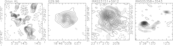
Figure 4.— Rotationally-torsionally excited CH₃OH$(7_{1,7}-6_{1,6})(v_{t}=1)$ images toward the four massive star-forming regions. Positive and negative features are shown as solid and dashed contours. The contouring is done from 15 to 95% (step 10%) of the peak emission, and the peak emission values are 7.5, 0.9, 1.0 and 0.6 Jy beam^-1 from left to right, respectively. The integration regimes for the four sources are [3,13], [91,105], [-58,-54] and [-18,-10] km s^-1. The grey-scale with dotted contours shows the submm continuum emission from Fig. 1. This figure is an adaption from the papers by Beuther et al. (2005a, 2007c, 2007d); Leurini et al. (2007). The axis are labeled in R.A. (J2000) and Dec. (J2000). The spatial resolution is listed in Table 2.

Toward G29.96, we detect most lines previously also observed toward Orion-KL, a few exceptions are the ³⁰SiO line, some of the vibrationally-torsionally state $v_{t}=2$ CH₃OH lines, some N-bearing molecular lines from larger molecules like CH₃CH₂CN or CH₃CHCN, as well as a few ³⁴SO₂ and HCOOCH₃ lines. While for some of the weaker lines this difference may partly be attributed to the larger distance of G29.96, for other lines such an argument is unlikely to hold. For example, the CH₃CH₂CN line at 348.55 GHz is stronger than the neighboring H₂CS line in Orion-KL whereas it remains undetected in G29.96 compared to the strong H₂CS line there. This is also reflected in the different abundance ratio of CH₃CH₂CN/H₂CS which is more than an order of magnitude larger in Orion-KL compared with G29.96 (see Table 4). Therefore, these differences are likely tracing true chemical variations between sources. In contrast, the only lines observed toward G29.96 but not detected toward Orion-KL are a few CH₃OCH₃ lines.

The main SiO isotopologue ²⁸SiO(8–7) is detected in all sources but IRAS 05358+3543. This is relatively surprising because SiO(2–1) is strong in this region (Beuther et al., 2002a), and the upper level energy of the $J=8-7$ of $\sim$75 K does not seem that extraordinarily high to produce a non-detection. For example, the detected CH₃OH$(7_{1,7}-6_{1,6})v_{t}=1$ transition has an upper level energy of 356 K. This implies that IRAS 05358+3543 does have warm molecular gas close to the central sources. However, the outflow-components traced by SiO are at on average lower temperatures (probably of the order 30 K, e.g., Cabrit & Bertout 1990) which may be the cause of the non-detection in IRAS 05358+3543. Furthermore, the critical density of the SiO(8–7) line is about two orders of magnitude higher than that of the (2–1) transition. Hence, the density structure of the core may cause the (8–7) non-detection in IRAS 05358+3543 as well.

While the rarer ³⁰SiO(8–7) isotopologue is detected toward Orion-KL with nearly comparable strength as the main isotopologue (Fig. 2 and Beuther et al. 2005a), we do not detect it at all in any of the other sources.

A little bit surprising, the H₂CS line at 338.081 GHz is detected toward Orion-KL, G29.96 as well as the lowest luminosity source IRAS 05358+3543, however, it remains undetected toward the more luminous HMPO IRAS 23151+5912. We are currently lacking a good explanation for this phenomenon because H₂CS is predicted by most chemistry networks as a parent molecule to be found early in the evolutionary sequence (e.g., Nomura & Millar 2004). The sulphur and nitrogen chemistries are also peculiar in this sample, and we outline some examples below.

3.2.4 Sulphur chemistry

The rare Carbon-sulphur isotopologue C³⁴S is detected toward all four regions (Fig. 2). However, as shown in Fig. 5 C³⁴S does not peak toward the main submm continuum peaks but is offset at the edge of the core. In the cases of G29.96 and IRAS 23151+5912 the C³⁴S morphology appears to wrap around the main submm continuum peaks. Toward IRAS 05358+3543 C³⁴S is also weak toward the strongest submm peak (at the eastern edge of the image) but shows the strongest C³⁴S emission features offset from a secondary submm continuum source (in the middle of the image). Toward Orion-KL, weak C³⁴S emission is detected in the vicinity of the hot core peak, whereas we find strong C³⁴S emission peaks offset from the dust continuum emission.

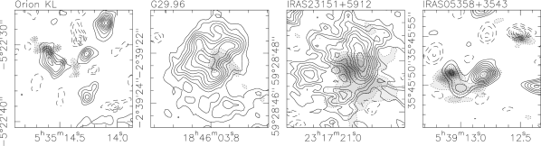
Figure 5.— C³⁴S(7–6) images toward the four massive star-forming regions. Positive and negative features are shown as solid and dashed contours. The contouring is done from 15 to 95% (step 10%) of the peak emission, and the peak emission values are 7.5, 0.9, 1.0 and 0.6 Jy beam^-1 from left to right, respectively. The integration regimes for the four sources are [-2,14], [92,104], [-58,-51] and [-17,-13] km s^-1. The grey-scale with dotted contours shows the submm continuum emission from Fig. 1. This figure is an adaption from the papers by Beuther et al. (2005a, 2007c, 2007d); Leurini et al. (2007). The axis are labeled in R.A. (J2000) and Dec. (J2000). The spatial resolution is listed in Table 2.

To check whether our optical-thin assumption from §3.2.2 is valid also for C³⁴S we ran LVG radiative transfer models (RADEX, van der Tak et al. 2007). We started with the H₂ column densities from Table 1 and assumed a typical CS/H₂ abundance of $10^{-8}$ with a terrestrial CS/C³⁴S ratio of 23 (Wannier, 1980). Above the critical density of $2\times 10^{7}$ cm^-3, with the given broad C³⁴S spectral FWHM (between 5 and 12 km s^-1 for the four sources), the C³⁴(7–6) emission is indeed optically thin. Hence optical depth effects are not causing these large offsets. Since furthermore the line intensities depend not just on the excitation but more strongly on the gas column densities, excitation effects only, as quantified in §3.2.1, cannot cause the observational offsets as well. Therefore, chemical evolution may be more important. A likely scenario is based on different desorption temperatures of molecules from dust grains (e.g., Viti et al. 2004): CS and C³⁴S are desorbed from grains at temperatures of a few 10 K, and at such temperatures, these molecules are expected to be well correlated with the dust continuum emission. Warming up further, at 100 K H₂O desorbs and then dissociates to OH. The OH quickly reacts with the sulphur forming SO and SO₂ which then will be centrally peaked (see §3.2.6). Toward G29.96, IRAS 23151+5912 and IRAS 05358+3543 we find that the SO₂ emission is centrally peaked toward the main submm continuum peaks confirming the above outlined chemical scenario (Fig. 6 & §3.2.6) . To further investigate the C³⁴S/SO₂ differences, we produced column density ratio maps between C³⁴S and SO₂ for G29.96, IRAS 23151+5912 and IRAS 05358+3543, assuming local thermodynamic equilibrium and optically thin emission (Fig. 7). To account for the spatial differences that SO₂ is observed toward the submm peak positions whereas C³⁴S is seen more to the edges of the cores, for the column density calculations we assumed the temperatures given in Table 1 for SO₂ whereas we used half that temperature for C³⁴S. Although the absolute ratio values are highly uncertain because of the different spatial filtering properties of the two molecules, qualitatively as expected, the column density ratio maps have the lowest values in the vicinity of the submm continuum sources and show increased emission at the core edges. The case is less clear for Orion-KL which shows the strongest SO₂ emission toward the south-eastern region called compact ridge. Since this compact ridge is believed to be caused by the interaction of a molecular outflow with the ambient dense gas (e.g., Liu et al. 2002) and SO₂ is known to be enriched by shock interactions with outflows, this shock-outflow interaction may dominate in Orion-KL compared with the above discussed C³⁴S/SO₂ scenario. For more details on the chemical evolution see the modeling in §3.2.6.

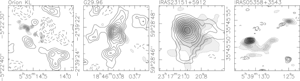
Figure 6.— SO${}_{2}(14_{4,14}-18_{3,15})$ images toward the four massive star-forming regions. Positive and negative features are shown as solid and dashed contours. The contouring is done from 15 to 95% (step 10%) of the peak emission, and the peak emission values are 7.5, 0.9, 1.0 and 0.6 Jy beam^-1 from left to right, respectively. Only for IRAS 05358+1732 the contouring starts at the 35% level because of a worse signal-to-noise ratio. The integration regimes for the four sources are [0,20], [94,100], [-60,-50] and [-17,-13] km s^-1. The grey-scale with dotted contours shows the submm continuum emission from Fig. 1. This figure is an adaption from the papers by Beuther et al. (2005a, 2007c, 2007d); Leurini et al. (2007). The axis are labeled in R.A. (J2000) and Dec. (J2000). The spatial resolution is listed in Table 2.

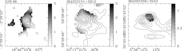
Figure 7.— Column density ratios between C³⁴S over SO₂ toward G29.96, IRAS 23151+5912 and IRAS 05358+3543 are shown in grey-scale. The contours present the corresponding submm continuum maps as in shown the previous figures. For IRAS 05358+3543 we zoom only into the central region to better show the ratio variations.

3.2.5 Nitrogen chemistry

It is intriguing that we do not detect any nitrogen-bearing molecule toward the two younger HMPOs IRAS 23151+5912 and IRAS 05358+3543 (Fig.2 and Table Chemical Diversity in High-Mass Star Formation). This already indicates that the nitrogen-chemistry needs warmer gas to initiate or requires more time to proceed. To get an idea about the more subtle variations of the nitrogen chemistry, one may compare some specific line pairs: For example, the HN¹³C/CH₃CH₂CN line blend (dominated by HN¹³C) and the SO₂ line between 348.3 and 348.4 GHz are of similar strength in the HMC Orion-KL (Fig. 2). The same is approximately true for the HMC G29.96, although SO₂ is relatively speaking a bit weaker there. The more interesting differences arise if one contrasts with the younger sources. Toward the $10^{5}$ L_⊙ early-HMPO IRAS 23151+5912, we only detect the SO₂ line and the HN¹³C/CH₃CH₂CN line blend remains a non-detection in this source. In the lower luminosity early-HMPO IRAS 05358+3543, both lines are not detected, although another SO₂ line at 338.3 GHz is detected there.

Judging from these line ratios, one can infer that SO₂ is relatively easy to excite early-on in the evolution of high-mass star-forming regions. Other sulphur-bearing molecules like H₂CS or CS are released even earlier from the grains, but SO-type molecules are formed quickly (e.g., Charnley 1997; Nomura & Millar 2004). In contrast to this, the non-detection of spectral lines like the HN¹³C/CH₃CH₂CN line blend in the early-HMPOs indicates that the formation and excitation of such nitrogen-bearing species takes place in an evolutionary more evolved phase. This may either be due to molecule-selective temperature-dependent gas-dust desorption processes or chemical network reactions requiring higher temperatures. Furthermore, simulations of chemical networks show that the complex nitrogen chemistry simply needs more time to be activated (e.g., Charnley et al. 2001; Nomura & Millar 2004). Recent modeling by Garrod et al. (2007) indicates that the gradual switch-on phase of hot molecular cores is an important evolutionary stage to produce complex molecules. In this picture, the HMCs have switched on their heating sources earlier and hence had more time to form these nitrogen molecules.

Comparing just the two HMCs, we find that the CH₃CH₂CN at 348.55 GHz is strong in Orion-KL but not detected in G29.96. Since G29.96 also exhibits less vibrationally-torsionally excited CH₃OH lines, it is likely on average still at lower temperatures than Orion-KL and may hence have not formed yet all the complex nitrogen-bearing molecules present already in Orion-KL.

3.2.6 Modeling

To examine the chemical evolution of warm regions in greater detail we used the chemical model of Bergin & Langer (1997).  This model includes gas-phase chemistry and the freeze-out to and sublimation from grain surfaces.   The details of this model are provided in that paper with the only addition being the inclusion of water ice formation on grain surfaces.  The binding energies we have adopted are for bare silicate grains, except for water ice which is assumed to have a binding energy appropriate for hydrogen bonding between frozen water molecules (Fraser et al., 2001). To explore the chemistry of these hot evaporative regions we have run the model for 10⁶ yrs with starting conditions at $n_{\rm H_{2}}=10^{6}$ cm^-3 and $T_{\rm{gas}}=T_{\rm{dust}}$=20 K.  Under these conditions most gaseous molecules, excluding H₂, will freeze onto the grain surface and the ice mantle forms, dominated by H₂O.    This timescale (10⁵ yrs ) is quite short, but is longer than the free-fall time at this density and is chosen as a representative time that gas might spend at very high density.  After completion we assume that a massive star forms and the gas and dust temperature is raised such that the ice mantle evaporates and the gas-phase chemistry readjusts. We have made one further adjustment to this model.  Our data suggest that HNC (a representative nitrogen-bearing species) is not detected in early-HMPOs and that the release of this species (or its pre-cursor) from the ice occurs during more evolved and warmer stages. Laboratory data  on ice desorption suggest that the process is not as simple as generally used in models where a given molecule evaporates at its sublimation temperature (Collings et al., 2004).  Rather some species co-desorb with water ice and the key nitrogen-bearing species, NH₃, falls into this category (see also Viti et al. 2004). We have therefore assumed that the ammonia evaporates at the same temperature as water ice.   Our initial abundances are taken from Aikawa et al. (1996), except we assume that 50% of the nitrogen is frozen in the form of NH₃ ice. This assumption is consistent with two sets of observations. First, detections of NH₃ in ices towards YSO’s find abundances of $\sim$ 2-7% relative to H₂O (Bottinelli et al., 2007). Dartois et al. (2002) find a limit of $\sim$ 5% relative to H₂O towards other YSO’s. Our assumed abundance of NH₃ ice is 5 $\times 10^{-6}$ relative to H₂O, assuming an ice abundance of 10^-4 (as appropriate for cold sources) this provides an ammonia ice abundance of $\sim$5%, which is consistent with ice observations. Second, high resolution ammonia observations often find high abundances of NH₃ in the gas phase towards hot cores, often as high as 10^-5, relative to H₂ (e.g., Cesaroni et al. 1994). Pure gas phase chemistry will have some difficulty making this high abundance in the cold phase and we therefore assume it is made on grains during cold phases.

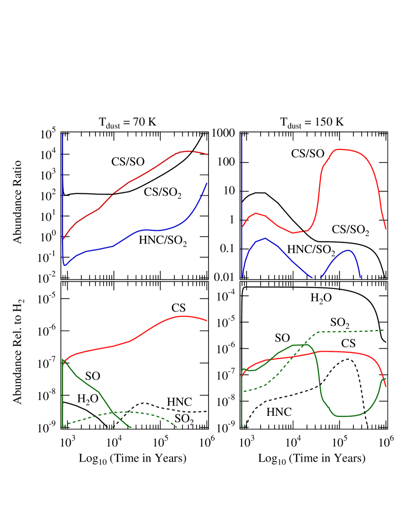
Figure 8.— The left and right columns show results from our modeling of the “cold and warm models”, respectively. The two top-panels show the abundance ratios between several species important for our observations versus the time. The bottom panels present the abundances relative to H₂. Time in this figure refers to time after the onset of massive star formation and hence we do not show any evolution during the cold starless phase.

Figure 8 presents our chemical model results at the point of star “turn on” where the gas and dust becomes warmer and ices evaporate.    Two different models were explored.  The first labeled as $T_{dust}$=70 K (“warm model”) is a model which is insufficient to evaporate water ice, while the second, “hot model” with $T_{dust}$=150 K, evaporates the entire ice mantle.   Much of the chemical variations amongst the early-HMPO and HMC phases is found for CS, SO, SO₂, and HNC (note this line is blended with CH₃CH₂CN) and we focus on these species in our plots (along with H₂O). It is also important to reiterate that due to differences in spatial sampling between the different sources as well as between line and continuum emission, we cannot derive accurate abundances from these data, but rather can attempt to use the models to explain trends. For the warm model the main result is that the imbalance created in the chemistry by the release of most species, with ammonia and water remaining as ices on the grains, leads to enhanced production of CS.   Essentially the removal of oxygen from the gas (excluding the O found in CO) allows for rapid CS production from the atomic Sulfur frozen on grains during the cold phase. Thus, for early-HMPOs, which might not have a large fraction of gas above the water sublimation point ($T\sim 110$ K), the ratios of CS to other species are quite large. In the hot model, when the temperature can evaporate both H₂O and NH₃ ice, ratios between the same molecules are orders of magnitude lower (Fig. 8). There is a large jump in the water vapor abundance (and NH₃, which is not shown) between the warm and the hot model driving the chemistry into new directions.  CS remains in the gas, but not with as high abundance as in the warm phase and is gradually eroded into SO and ultimately SO₂. Hence, SO₂ appears to be a better tracer of more evolved stages. In this sense, even the early-HMPOs can be considered as relatively evolved, and it will be important to extend similar studies to even earlier evolutionary stages.  HNC also appears as a brief intermediate product of the nitrogen chemistry.

The above picture is in qualitative agreement with our observations: that CS should be a good tracer in early evolutionary states even prior to our observed sample, but that it is less well suited for more evolved regions like those studied here. Other sulfur-bearing molecules, in particular SO₂, appear to better trace the warmest gas near the forming star.   HNC, and perhaps other nitrogen-bearing species, are better tracers when the gas is warm enough to evaporate a significant amount of the ice mantle.

3.3. Searching for disk signatures

While the chemical evolution of massive star-forming regions is interesting in itself, one also wants to use the different characteristics of molecular lines as tools to trace various physical processes. While molecules like CO or SiO have regularly been used to investigate molecular outflows (e.g., Arce et al. 2007), the problem to identify the right molecular tracer to investigate accretion disks in massive star formation is much more severe (e.g., Cesaroni et al. 2007). Major observational obstacles arise from the fact that disk-tracing molecular lines are usually often not unambiguously found only in the accretion disk, but that other processes can produce such line emission as well. For example, molecular lines from CN and HCN are high-density tracers and were believed to be good candidates to investigate disks in embedded protostellar sources (e.g., Aikawa & Herbst 2001). However, observations revealed that both spectral lines are strongly affected by the associated molecular outflow and hence difficult to use for massive disk studies (CN Beuther et al. 2004a, HCN Zhang et al. 2007).

As presented in Cesaroni et al. (2007), various different molecules have in the past been used to investigate disks/rotational signatures in massive star formation (e.g., CH₃CN, C³⁴S, NH₃, HCOOCH₃, C¹⁷O, H${}_{2}^{18}$O, see also Fig. 9). The data presented here add three other potential disk tracers (HN¹³C and HC₃N for G29.96, Beuther et al. 2007c, and torsionally excited CH₃OH for IRAS 23151+5912 and IRAS 05358+3543 Beuther et al. 2007d; Leurini et al. 2007, Fig. 9). An important point to note is that in most sources only one or the other spectral line exclusively allows a study of rotational motions, whereas other lines apparently do not trace the warm disks. For example, C³⁴S traces the Keplerian motion in the young source IRAS 20126+4104 whereas it does not trace the central protostars at all in the sources presented here (Fig. 5). In the contrary, HN¹³C shows rotational signatures in the HMC G29.96, but it remains completely undetected in the younger early-HMPO sources of our sample (Figs. 9 & 2). As discussed in sections 3.2.4 and 3.2.5, this implies that, depending on the chemical evolution, molecules like C³⁴S should be better suited for disk studies at very early evolutionary stages, whereas complex nitrogen-bearing molecules are promising in more evolved hot-core-type sources. While the chemical evolution is important for these molecules, temperature effects have to be taken into account as well. For example, the torsionally excited CH₃OH line traces rotating motions in IRAS 23151+5912 and IRAS 05358+3543 (Beuther et al. 2007d; Leurini et al. 2007, Fig. 9) but it is weak and difficult to detect in colder and younger sources. Therefore, some initial heating is required to employ highly excited lines for kinematic studies. In addition to these evolutionary effects, optical depth is important for many lines. For example, Cesaroni et al. (1997, 1999) have shown that CH₃CN traces the rotating structure in IRAS 20126+4104, whereas the same molecule does not indicate any rotation in IRAS 18089-1732 (Beuther et al., 2005b). A likely explanation for the latter is high optical depth of the CH₃CN submm lines (Beuther et al., 2005b). Again other molecules are excited in the accretion disks as well as the surrounding envelope, causing confusion problems to disentangle the various physical components. In summary, getting a chemical rich spectral line census like the ones presented here shows that one can find several disk-tracing molecules in different sources, but it also implies that some previously assumed good tracers are not necessarily universally useful.

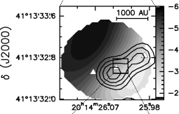
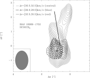
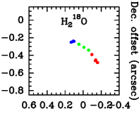
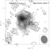
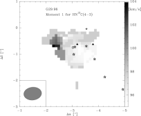
Figure 9.— Examples of rotation-tracing molecules: top-left: C³⁴S in IRAS 20126+4104 (Cesaroni et al., 1999, 2005), top-middle: HCOOCH₃ in IRAS 18089-1732 (Beuther et al., 2005b), top-right: H${}_{2}^{18}$O in AFGL2591 (van der Tak et al., 2006), bottom-left: CH₃OH $v_{t}=1$ in IRAS 23151+5912 (Beuther et al., 2007d), bottom-right: HN¹³C in G29.96 (Beuther et al., 2007c).

The advent of broad bandpass interferometers like the SMA now fortunately allows to observe many molecular lines simultaneously. This way, one often finds a suitable rotation-tracing molecule in an observational spectral setup. Nevertheless, one has to keep in mind the chemical and physical complexity in such regions, and it is likely that in many cases only combined modeling of infall, rotation and outflow will disentangle the accretion disk from the rest of the star-forming gas and dust core.

4. Conclusion and Summary

We compiled a sample of four massive star-forming regions in different evolutionary stages with varying luminosities that were observed in exactly the same spectral setup at high angular resolution with the SMA. We estimated column densities for all sources and detected species, and we compared the spatial distributions of the molecular gas. This allows us to start investigating chemical evolutionary effects also in a spatially resolved manner. Chemical modeling was conducted to explain our observations in more detail.

A general result from this comparison is that many different physical and chemical processes are important to produce the complex chemical signatures we observe. While some features, e.g., the non-detection of the rich vibrationally-torsionally excited CH₃OH line forest toward the two early-HMPOs can be explained by on average lower temperatures of the molecular gas compared to the more evolved HMCs, other observational characteristics require chemical evolutionary sequences caused by heating including grain-surface and gas phase reactions. Even other features are then better explained by shock-induced chemical networks.

The rare isotopologue C³⁴S is usually not detected right toward the main submm continuum peaks, but rather at the edge of the star-forming cores. This may be explained by temperature-selective gas-desorption processes and successive gas chemistry networks. Furthermore, we find some nitrogen-bearing molecular lines to be only present in the HMCs, whereas they remain undetected at earlier evolutionary stages. This indicates that the formation and excitation of many nitrogen-bearing molecules needs considerably higher temperatures and/or more time during the warm-up phase of the HMC, perhaps relating to the fact that NH₃ is bonded within the water ice mantle. Although the statistical database is still too poor to set tighter constraints, these observations give the direction how one can use the presence and morphology of various molecular lines to identify and study different (chemical) evolutionary sequences.

Furthermore, we discussed the observational difficulty to unambiguously use one or the other spectral line as a tracer of massive accretion disks. While some early spectral line candidates are discarded for such kind of studies by now (e.g., CN), in many other sources we find different lines exhibiting rotational velocity signatures. The observational feature that in most sources apparently only one or the other spectral line exclusively traces the desired structures has likely to be attributed to a range of effects. (1) Chemical effects, where for example C³⁴S may work in the youngest sources whereas some nitrogen-bearing molecules like HN¹³C are better in typical HMCs. (2) Confusion from multiple gas components, mainly outflows, infall from the envelope and rotation. (3) High optical depth from many molecular lines. This implies that for future statistical studies we have to select spectral setups that comprise many molecular lines from various species. This way, one has good chances to identify for each source separately the right molecular tracer, and hence still draw statistically significant conclusions.

To advance in this field and to become more quantitative, different steps are necessary. First of all, we need to establish a larger database of more sources at different evolutionary stages, in particular even younger sources, as well as with varying luminosities to better characterize the differences and similarities. From an observational and technical point of view, although the presented data are state of the art multi-wavelength and high angular resolution observations, the quantitative interpretation is still hampered by the spatial filtering of the interferometer. To become more quantitative, it is therefore necessary to complement such data with the missing short spacing information. While we have high angular resolution in all datasets with a similar baseline coverage and hence similarly covered angular scales, the broad range of distances causes a different coverage of sampled linear spatial scales. Hence the missing short spacings affect each dataset in a different fashion which is currently the main limiting factor for a better quantitative interpretation of the data. Therefore, obtaining single-dish observations in the same spectral setup and then combining them with the SMA observations is a crucial step to derive more reliable column densities and from that abundances. These parameters then can be used by theorists to better model the chemical networks, explain the observations and predict other suitable molecules for, e.g., massive disk studies.

[htb]lrrcccc Line peak intensities $S_{\rm{peak}}$ and upper state energy levels $E_{u}/k$ from spectra toward peak positions of the respective massive star-forming regions (Fig. 2).
Freq. Line $E_{u}/k$ $S_{\rm{peak}}$ $S_{\rm{peak}}$ $S_{\rm{peak}}$ $S_{\rm{peak}}$
(GHz) (K) (Jy) (Jy) (Jy) (Jy)
Orion G29.96 23151 05358
337.252 CH₃OH$(7_{3,5}-6_{3,4})$A($v_{t}$=2) 739 6.0
337.274 CH₃OH$(7_{4,3}-6_{4,2})$A($v_{t}$=2) 695 7.4
337.279 CH₃OH$(7_{2,5}-6_{2,4})$E($v_{t}$=2) 727 5.4
337.284 CH₃OH$(7_{0,7}-6_{0,6})$A($v_{t}$=2) 589 9.9
337.297 CH₃OH$(7_{1,7}-6_{1,6})$A($v_{t}$=1) 390 10.6 1.7
337.312 CH₃OH$(7_{1,6}-6_{1,5})$E($v_{t}$=2) 613 9.2
337.348 CH₃CH₂CN$(38_{3,36}-37_{3,35})$ 328 14.2 1.5
337.397 C³⁴S(7–6) 65 12.6 2.0 0.3 0.6
337.421 CH₃OCH${}_{3}(21_{2,19}-20_{3,18})$ 220 3.0 0.6
337.446 CH₃CH₂CN$(37_{4,33}-36_{4,32})$ 322 11.2 0.8
337.464 CH₃OH$(7_{6,1}-6_{0,0})$A($v_{t}$=1) 533 7.2 1.1
337.474 UL 4.9 0.6
337.490 HCOOCH${}_{3}(27_{8,20}-26_{8,19})$E 267 6.3 0.7
337.519 CH₃OH$(7_{5,2}-6_{5,2})$E($v_{t}$=1) 482 8.1 1.0
337.546 CH₃OH$(7_{5,3}-6_{5,2})$A($v_{t}$=1) 485 10.0^b 1.4^b
CH₃OH$(7_{5,2}-6_{5,1})$A^-($v_{t}$=1) 485 10.0^b 1.4^b
337.582 ³⁴SO$(8_{8}-7_{7})$ 86 12.2 2.0 1.1
337.605 CH₃OH$(7_{2,5}-6_{2,4})$E($v_{t}$=1) 429 9.7 2.4
337.611 CH₃OH$(7_{6,1}-6_{6,0})$E($v_{t}$=1) 657 6.2^b 2.0^b
CH₃OH$(7_{3,4}-6_{3,3})$E($v_{t}$=1) 388 6.2^b 2.0^b
337.626 CH₃OH$(7_{2,5}-6_{2,4})$A($v_{t}$=1) 364 11.0 1.9
337.636 CH₃OH$(7_{2,6}-6_{2,5})$A^-($v_{t}$=1) 364 8.2 2.5
337.642 CH₃OH$(7_{1,7}-6_{1,6})$E($v_{t}$=1) 356 10.9^b 2.9^b 0.6^b 1.1^b
337.644 CH₃OH$(7_{0,7}-6_{0,6})$E($v_{t}$=1) 365 10.9^b 2.9^b 0.6^b 1.1^b
337.646 CH₃OH$(7_{4,3}-6_{4,2})$E($v_{t}$=1) 470 10.9^b 2.9^b 0.6^b 1.1^b
337.648 CH₃OH$(7_{5,3}-6_{5,2})$E($v_{t}$=1) 611 10.9^b 2.9^b 0.6^b 1.1^b
337.655 CH₃OH$(7_{3,5}-6_{3,4})$A($v_{t}$=1) 461 10.8^b 2.0^b
CH₃OH$(7_{3,4}-6_{3,3})$A^-($v_{t}$=1) 461 10.8^b 2.0^b
337.671 CH₃OH$(7_{2,6}-6_{2,5})$E($v_{t}$=1) 465 10.2 2.1
337.686 CH₃OH$(7_{4,3}-6_{4,2})$A($v_{t}$=1) 546 9.^b5 2.0^b
CH₃OH$(7_{4,4}-6_{4,3})$A^-($v_{t}$=1) 546 9.5^b 2.0^b
CH₃OH$(7_{5,2}-6_{5,1})$E($v_{t}$=1) 494 9.5^b 2.0^b
337.708 CH₃OH$(7_{1,6}-6_{1,5})$E($v_{t}$=1) 489 7.9 1.8
337.722 CH₃OCH${}_{3}(7_{4,4}-6_{3,3})$EE 48 0.9
337.732 CH₃OCH${}_{3}(7_{4,3}-6_{3,3})$EE 48 1.4
337.749 CH₃OH$(7_{0,7}-6_{0,6})$A($v_{t}$=1) 489 8.7 1.9
337.778 CH₃OCH${}_{3}(7_{4,4}-6_{3,4})$EE 48 1.3
337.787 CH₃OCH${}_{3}(7_{4,3}-6_{3,4})$AA 48 1.4
337.825 HC₃N$(37-36)v_{7}=1$ 629 14.8 1.4
337.838 CH₃OH$(20_{6,14}-21_{5,16})$E 676 5.6 1.1
337.878 CH₃OH$(7_{1,6}-6_{1,5})$A($v_{t}$=2) 748 2.7 0.6
337.969 CH₃OH$(7_{1,6}-6_{1,5})$A($v_{t}$=1) 390 12.0 2.1
338.081 H₂CS$(10_{1,10}-9_{1,9})$ 102 5.8 2.3 0.5
338.125 CH₃OH$(7_{0,7}-6_{0,6})$E 78 6.9 2.8 1.4 1.9
338.143 CH₃CH₂CN$(37_{3,34}-36_{3,33})$ 317 14.4 0.9
338.214 CH₂CHCN$(37_{1,37}-36_{1,36})$ 312 4.0
338.306 SO${}_{2}(18_{4,1}-18_{3,1})$ 197 x^c 0.8 1.2 0.7
338.345 CH₃OH$(7_{1,7}-6_{1,6})$E 71 13.4 2.1 1.3 2.3
338.405 CH₃OH$(7_{6,2}-6_{6,1})$E 244 13.1^b 3.0^b
338.409 CH₃OH$(7_{0,7}-6_{0,6})$A 65 13.1^b 3.0^b 1.5 2.4
338.431 CH₃OH$(7_{6,1}-6_{6,0})$E 254 9.5 1.8
338.442 CH₃OH$(7_{6,1}-6_{6,0})$A 259 11.7^b 2.7^b 0.5^b
CH₃OH$(7_{6,2}-6_{6,1})$A^- 259 11.7^b 2.7^b 0.5^b
338.457 CH₃OH$(7_{5,2}-6_{5,1})$E 189 8.9 2.0 0.4 0.6
338.475 CH₃OH$(7_{5,3}-6_{5,2})$E 201 12.6 2.5 0.5
338.486 CH₃OH$(7_{5,3}-6_{5,2})$A 203 9.4^b 2.3^b 0.8^b 0.8^b
CH₃OH$(7_{5,2}-6_{5,1})$A^- 203 9.4^b 2.3^b 0.8^b 0.8^b
338.504 CH₃OH$(7_{4,4}-6_{4,3})$E 153 8.5 2.7 0.7 0.7
338.513 CH₃OH$(7_{4,4}-6_{4,3})$A^- 145 13.7^b 2.8^b 1.4^b 1.3^b
CH₃OH$(7_{4,3}-6_{4,2})$A 145 13.7^b 2.8^b 1.4^b 1.3^b
CH₃OH$(7_{2,6}-6_{2,5})$A^- 103 13.7^b 2.8^b 1.4^b 1.3^b
338.530 CH₃OH$(7_{4,3}-6_{4,2})$E 161 5.8 2.7 0.7 0.9
338.541 CH₃OH$(7_{3,5}-6_{3,4})$A⁺ 115 12.5^b 3.0^b 2.0^b 1.4^b
338.543 CH₃OH$(7_{3,4}-6_{3,3})$A^- 115 12.5^b 3.0^b 2.0^b 1.4^b
338.560 CH₃OH$(7_{3,5}-6_{3,4})$E 128 15.6 2.5 0.9 0.6
338.583 CH₃OH$(7_{3,4}-6_{3,3})$E 113 11.5 3.4 1.0 1.1
338.612 SO${}_{2}(20_{1,19}-19_{2,18})$ 199 x^c 2.9 1.5 1.9
338.615 CH₃OH$(7_{1,6}-6_{1,5})$E 86 x^d 2.9^d 1.5^d 1.9^d
338.640 CH₃OH$(7_{2,5}-6_{2,4})$A 103 7.2 2.5 1.0 1.0
338.722 CH₃OH$(7_{2,5}-6_{2,4})$E 87 10.2^b 3.2^b 2.1^b 2.7^b
338.723 CH₃OH$(7_{2,6}-6_{2,5})$E 91 10.2^b 3.2^b 2.1^b 2.7^b
338.760 ¹³CH₃OH$(13_{7,7}-12_{7,6})$A 206 4.0 1.1
338.769 HC₃N$(37-36)v_{7}=2$ 525 ? ?
338.786 ³⁴SO${}_{2}(14_{4,10}-14_{3,1})$ 134 6.2
338.886 C₂H₅OH$(15_{7,8}-15_{6,19})$ 162 5.3 0.8
338.930 ³⁰SiO(8–7) 73 24.4
339.058 C₂H₅OH$(14_{7,7}-14_{6,8})$ 150 x^e 0.6
347.232 CH₂CHCN$(38_{1,38}-37_{1,37})$ 329 4.9 0.6
347.331 ²⁸SiO(8–7) 75 22.1 0.9 0.7
347.438 UL 7.5
347.446 UL 3.4 0.8
347.478 HCOOCH${}_{3}(27_{1,26}-26_{1,25})$E 247 4.8
347.494 HCOOCH${}_{3}(27_{5,22}-26_{5,21})$A 247 2.9 0.6
347.590 HCOOCH${}_{3}(16_{6,10}-15_{5,11})$A 104 2.4
347.599 HCOOCH${}_{3}(16_{6,10}-15_{5,11})$E 105 1.7
347.617 HCOOCH${}_{3}(28_{10,19}-27_{10,18})$A 307 2.6
347.628 HCOOCH${}_{3}(28_{10,19}-27_{10,18})$E 307 3.6
347.667 UL 4.5
347.759 CH₂CHCN$(36_{2,34}-35_{2,32})$ 317 8.3 0.7
347.792 UL 5.4 0.7
347.842 UL, ¹³CH₃OH 3.1 0.5
347.916 C₂H₅OH$(20_{4,17}-19_{4,16})$ 251 3.3 0.7
347.983 UL 0.6
348.050 HCOOCH${}_{3}(28_{4,24}-27_{4,23})$E 266 2.8
348.066 HCOOCH${}_{3}(28_{6,23}-27_{6,22})$A 266 3.0
348.118 ³⁴SO${}_{2}(19_{4,16}-19_{3,17})$ 213 5.8
348.261 CH₃CH₂CN$(39_{2,37}-38_{2,36})$ 344 11.2 1.2
348.340 HN¹³C(4–3) 42 16.1^b 2.0^b
348.345 CH₃CH₂CN$(40_{2,39}-39_{2,38})$ 351 16.1^b 2.0^b
348.388 SO${}_{2}(24_{2,22}-23_{3,21})$ 293 9.3 0.5 1.0
348.518 UL, HNOS$(1_{1,1}-2_{0,2})$ 10.6 0.7
348.532 H₂CS$(10_{1,9}-9_{1,8})$ 105 7.4 1.9
348.553 CH₃CH₂CN$(40_{1,39}-39_{1,38})$ 351 20.1
348.910 HCOOCH${}_{3}(28_{9,20}-27_{9,19})$E 295 11.0^b 1.6^b
348.911 CH₃CN$(19_{9}-18_{9})$ 745 11.0^b 1.6^b
348.991 CH₂CHCN$(37_{1,36}-36_{1,35})$ 325 5.9
349.025 CH₃CN$(19_{8}-18_{8})$ 624 9.5 1.1
349.107 CH₃OH$(14_{1,13}-14_{0,14})$ 43 12.2 3.1 1.3 1.1
^a Doubtful detection since other close $v_{t}=2$ lines with similar upper
energy levels were not detected.
^b Line blend.
^c No flux measurement possible because averaged over the given 5700 AU negative
features due to missing short spacings overwhelm the positive features (see Figs. 3 & 6).
^d Peak flux corrupted by neighboring SO₂ line.
^e Only detectable with higher spatial resolution (Beuther et al., 2005a).

Table 4Molecular column densities.

	Orion-KLa	G29.96	23151	05358
CH3OH	$2{\sf x}10^{16}$	$4{\sf x}10^{17}\,{}^{b}$	$3{\sf x}10^{16}-1{\sf x}10^{17}\,{}^{c}$	$4{\sf x}10^{15}-4{\sf x}10^{18}\,{}^{d}$
CH3CH2CN	$5{\sf x}10^{15}$	$1{\sf x}10^{16}$	–	–
CH2CHCN	$5{\sf x}10^{15}$	$7{\sf x}10^{15}$	–	–
C34S	$2{\sf x}10^{14}$	$2{\sf x}10^{15}$	$2{\sf x}10^{14}$	$6{\sf x}10^{13}$
CH3OCH3	$1{\sf x}10^{16}$	$2{\sf x}10^{17}\,{}^{e}$	–	–
HCOOCH3	$6{\sf x}10^{15}$	$8{\sf x}10^{16}$	–	–
34SO	$6{\sf x}10^{14}$	$1{\sf x}10^{16}$	$4{\sf x}10^{15}$	–
SO2	$2{\sf x}10^{15}$	$3{\sf x}10^{16}$	$3{\sf x}10^{16}$	$1{\sf x}10^{16}\,{}^{d}$
HC3N	$6{\sf x}10^{14}$	$2{\sf x}10^{15}$	–	–
HN13C	blend	blend	–	–
H2CS	$4{\sf x}10^{14}$	$2{\sf x}10^{16}$	–	$4{\sf x}10^{14}$
C2H5OH	$2{\sf x}10^{15}$	$6{\sf x}10^{16}$	–	–
SiO	$2{\sf x}10^{14}$	$4{\sf x}10^{14}$	$2{\sf x}10^{14}$	–
CH3CN	$2{\sf x}10^{15}$	$1{\sf x}10^{16}$	–	$8{\sf x}10^{16}\,{}^{d}$

^a Calculated for lower average $T$ of 200 K because of smoothing to 5700 AU resolution (Figs. 2 & 3). The source size was approximated by half the spatial resolution. The on average lower Orion-KL column densities are likely due to the largest amount of missing flux for the closest source of the sample.
^b From Beuther et al. (2007c).
^c From Beuther et al. (2007d) for different sub-sources.
^d From Leurini et al. (2007) for different sub-sources.
^e At lower temperature of 100 K, because otherwise different lines would get excited.

References

- Aikawa & Herbst (2001) Aikawa, Y. & Herbst, E. 2001, A&A, 371, 1107
- Aikawa et al. (1996) Aikawa, Y., Miyama, S. M., Nakano, T., & Umebayashi, T. 1996, ApJ, 467, 684
- Arce et al. (2007) Arce, H. G., Shepherd, D., Gueth, F., et al. 2007, in Protostars and Planets V, ed. B. Reipurth, D. Jewitt, & K. Keil, 245–260
- Bergin & Langer (1997) Bergin, E. A. & Langer, W. D. 1997, ApJ, 486, 316
- Beuther et al. (2007a) Beuther, H., Churchwell, E. B., McKee, C. F., & Tan, J. C. 2007a, in Protostars and Planets V, ed. B. Reipurth, D. Jewitt, & K. Keil, 165–180
- Beuther et al. (2007b) Beuther, H., Leurini, S., Schilke, P., et al. 2007b, A&A, 466, 1065
- Beuther et al. (2002a) Beuther, H., Schilke, P., Gueth, F., et al. 2002a, A&A, 387, 931
- Beuther et al. (2002b) Beuther, H., Schilke, P., Menten, K. M., et al. 2002b, ApJ, 566, 945
- Beuther et al. (2004a) Beuther, H., Schilke, P., & Wyrowski, F. 2004a, ApJ, 615, 832
- Beuther et al. (2007c) Beuther, H., Zhang, Q., Bergin, E. A., et al. 2007c, A&A, 468, 1045
- Beuther et al. (2004b) Beuther, H., Zhang, Q., Greenhill, L. J., et al. 2004b, ApJ, 616, L31
- Beuther et al. (2005a) Beuther, H., Zhang, Q., Greenhill, L. J., et al. 2005a, ApJ, 632, 355
- Beuther et al. (2007d) Beuther, H., Zhang, Q., Hunter, T. R., Sridharan, T. K., & Bergin, E. A. 2007d, A&A, 473, 493
- Beuther et al. (2005b) Beuther, H., Zhang, Q., Sridharan, T. K., & Chen, Y. 2005b, ApJ, 628, 800
- Bisschop et al. (2007) Bisschop, S. E., Jørgensen, J. K., van Dishoeck, E. F., & de Wachter, E. B. M. 2007, A&A, 465, 913
- Blake et al. (1987) Blake, G. A., Sutton, E. C., Masson, C. R., & Phillips, T. G. 1987, ApJ, 315, 621
- Bottinelli et al. (2007) Bottinelli, S., Boogert, A. C. A., van Dishoeck, E. F., et al. 2007, in Molecules in Space and Laboratory
- Brogan et al. (2007) Brogan, C. L., Chandler, C. J., Hunter, T. R., Shirley, Y. L., & Sarma, A. P. 2007, ApJ, 660, L133
- Cabrit & Bertout (1990) Cabrit, S. & Bertout, C. 1990, ApJ, 348, 530
- Caselli et al. (1993) Caselli, P., Hasegawa, T. I., & Herbst, E. 1993, ApJ, 408, 548
- Cesaroni et al. (1994) Cesaroni, R., Churchwell, E., Hofner, P., Walmsley, C. M., & Kurtz, S. 1994, A&A, 288, 903
- Cesaroni et al. (1999) Cesaroni, R., Felli, M., Jenness, T., et al. 1999, A&A, 345, 949
- Cesaroni et al. (1997) Cesaroni, R., Felli, M., Testi, L., Walmsley, C. M., & Olmi, L. 1997, A&A, 325, 725
- Cesaroni et al. (2007) Cesaroni, R., Galli, D., Lodato, G., Walmsley, C. M., & Zhang, Q. 2007, in Protostars and Planets V, ed. B. Reipurth, D. Jewitt, & K. Keil, 197–212
- Cesaroni et al. (2005) Cesaroni, R., Neri, R., Olmi, L., et al. 2005, A&A, 434, 1039
- Charnley (1997) Charnley, S. B. 1997, ApJ, 481, 396
- Charnley et al. (2001) Charnley, S. B., Rodgers, S. D., & Ehrenfreund, P. 2001, A&A, 378, 1024
- Collings et al. (2004) Collings, M. P., Anderson, M. A., Chen, R., et al. 2004, MNRAS, 354, 1133
- Dartois et al. (2002) Dartois, E., d’Hendecourt, L., Thi, W., Pontoppidan, K. M., & van Dishoeck, E. F. 2002, A&A, 394, 1057
- Doty et al. (2006) Doty, S. D., van Dishoeck, E. F., & Tan, J. C. 2006, A&A, 454, L5
- Doty et al. (2002) Doty, S. D., van Dishoeck, E. F., van der Tak, F. F. S., & Boonman, A. M. S. 2002, A&A, 389, 446
- Fraser et al. (2001) Fraser, H. J., Collings, M. P., McCoustra, M. R. S., & Williams, D. A. 2001, MNRAS, 327, 1165
- Garrod et al. (2007) Garrod, R. T., Wakelam, V., & Herbst, E. 2007, A&A, 467, 1103
- Hatchell et al. (1998) Hatchell, J., Thompson, M. A., Millar, T. J., & MacDonald, G. H. 1998, A&AS, 133, 29
- Hildebrand (1983) Hildebrand, R. H. 1983, QJRAS, 24, 267
- Ho et al. (2004) Ho, P. T. P., Moran, J. M., & Lo, K. Y. 2004, ApJ, 616, L1
- Johnstone et al. (2003) Johnstone, D., Boonman, A. M. S., & van Dishoeck, E. F. 2003, A&A, 412, 157
- Krumholz et al. (2007) Krumholz, M. R., Klein, R. I., & McKee, C. F. 2007, ApJ, 656, 959
- Leurini et al. (2007) Leurini, S., Beuther, H., Schilke, P., et al. 2007, A&A, 475, 925
- Liu et al. (2002) Liu, S., Girart, J. M., Remijan, A., & Snyder, L. E. 2002, ApJ, 576, 255
- Müller et al. (2001) Müller, H. S. P., Thorwirth, S., Roth, D. A., & Winnewisser, G. 2001, A&A, 370, L49
- MacDonald et al. (1996) MacDonald, G. H., Gibb, A. G., Habing, R. J., & Millar, T. J. 1996, A&AS, 119, 333
- McCutcheon et al. (2000) McCutcheon, W. H., Sandell, G., Matthews, H. E., et al. 2000, MNRAS, 316, 152
- Menten & Reid (1995) Menten, K. M. & Reid, M. J. 1995, ApJ, 445, L157
- Millar et al. (1997) Millar, T. J., MacDonald, G. H., & Gibb, A. G. 1997, A&A, 325, 1163
- Mueller et al. (2002) Mueller, K. E., Shirley, Y. L., Evans, N. J., & Jacobson, H. R. 2002, ApJS, 143, 469
- Nomura & Millar (2004) Nomura, H. & Millar, T. J. 2004, A&A, 414, 409
- Olmi et al. (2003) Olmi, L., Cesaroni, R., Hofner, P., et al. 2003, A&A, 407, 225
- Poynter & Pickett (1985) Poynter, R. L. & Pickett, H. M. 1985, Appl. Opt., 24, 2235
- Schilke et al. (1997) Schilke, P., Groesbeck, T. D., Blake, G. A., & Phillips, T. G. 1997, ApJS, 108, 301
- Sridharan et al. (2002) Sridharan, T. K., Beuther, H., Schilke, P., Menten, K. M., & Wyrowski, F. 2002, ApJ, 566, 931
- Thompson et al. (2006) Thompson, M. A., Hatchell, J., Walsh, A. J., MacDonald, G. H., & Millar, T. J. 2006, A&A, 453, 1003
- van der Tak et al. (2007) van der Tak, F. F. S., Black, J. H., Schöier, F. L., Jansen, D. J., & van Dishoeck, E. F. 2007, A&A, 468, 627
- van der Tak et al. (2003) van der Tak, F. F. S., Boonman, A. M. S., Braakman, R., & van Dishoeck, E. F. 2003, A&A, 412, 133
- van der Tak et al. (2000) van der Tak, F. F. S., van Dishoeck, E. F., & Caselli, P. 2000, A&A, 361, 327
- van der Tak et al. (2006) van der Tak, F. F. S., Walmsley, C. M., Herpin, F., & Ceccarelli, C. 2006, A&A, 447, 1011
- van Dishoeck & Blake (1998) van Dishoeck, E. F. & Blake, G. A. 1998, ARA&A, 36, 317
- Viti et al. (2004) Viti, S., Collings, M. P., Dever, J. W., McCoustra, M. R. S., & Williams, D. A. 2004, MNRAS, 354, 1141
- Wakelam et al. (2005) Wakelam, V., Selsis, F., Herbst, E., & Caselli, P. 2005, A&A, 444, 883
- Wannier (1980) Wannier, P. G. 1980, ARA&A, 18, 399
- Wright et al. (1996) Wright, M. C. H., Plambeck, R. L., & Wilner, D. J. 1996, ApJ, 469, 216
- Wyrowski et al. (1999) Wyrowski, F., Schilke, P., Walmsley, C. M., & Menten, K. M. 1999, ApJ, 514, L43
- Yorke & Sonnhalter (2002) Yorke, H. W. & Sonnhalter, C. 2002, ApJ, 569, 846
- Zhang et al. (2007) Zhang, Q., Sridharan, T. K., Hunter, T. R., et al. 2007, A&A, 470, 269
- Zinnecker & Yorke (2007) Zinnecker, H. & Yorke, H. W. 2007, ARA&A, 45, 481