Diffusion Monte Carlo study of a valley degenerate electron gas and application to quantum dots

Abstract

A many-flavor electron gas (MFEG) in a semiconductor with a valley degeneracy ranging between 6 and 24 was analyzed using diffusion Monte Carlo (DMC) calculations. The DMC results compare well with an analytic expression derived by one of us [Phys. Rev. B 78, 035111 (2008)] for the total energy to within $\pm 1\,\%$ over an order of magnitude range of density, which increases with valley degeneracy. For $\text{Bi}_{2}\text{Te}_{3}$ (six-fold valley degeneracy) the applicable charge carrier densities are between $7\times 10^{19}\,\text{cm}^{-3}$ and $2\times 10^{20}\,\text{cm}^{-3}$. DMC calculations distinguished between an exact and a useful approximate expression for the 24-fold degenerate MFEG polarizability for wave numbers $2p_{\text{F}}<q<7p_{\text{F}}$. The analytical result for the MFEG is generalized to inhomogeneous systems by means of a gradient correction, the validity range of this approach is obtained. Employed within a density-functional theory calculation this approximation compares well with DMC results for a quantum dot.

I Introduction

Good quantum numbers, that describe conserved quantities as a quantum system evolves, derive their significance from their connection to the powerful conservation laws of physics. In addition to the familiar examples of spin and crystal momentum, under some circumstances electrons in solids can have an additional quantum number that distinguishes them, which we call the flavor; we denote the total number of flavors by $\nu$. One example of such a system are semiconductors and semimetals that have degenerate conduction-band valleys, the flavor denotes the electron’s valley. Examples of multi-valley semiconductors include Ge, which as shown in Fig. 1 has four degenerate valleys (N.B. not eight, as valleys at the Brillouin zone vertices overlap), Si has six degenerate valleys, a Ge-Si alloy has ten degenerate valleys, and $\text{Pb}_{1-x-y}\text{Sn}_{x}\text{Mn}_{y}\text{Te}$ has twelve valleys in the $\Sigma$ band Story et al. (1990). The system has been experimentally realized as an electron-hole liquid that forms in drops Andryushin et al. (1976); Conduit (2008). In these systems the number of flavors (the number of valleys) is well defined and there are strong Coulomb interactions between particles which motivates the analysis. This is in contrast to several other systems in which the number of flavors is poorly defined such as heavy fermions Zaránd et al. (2002); Kim (2005); Bolech and Iucci (2006), charged domain walls Eskes et al. (1998), a super-strong magnetic field Keldysh and Onishchenko (1976), and spin instabilities Giuliani and Quinn (1986); Marinescu et al. (2000); or where the number of flavors is well defined but interactions between particles are weak such as ultracold atoms in optical lattices Honerkamp and Hofstetter (2004a, b); Cherng et al. (2007).

The properties of a many-flavor electron gas (MFEG) in a semiconductor were first studied analytically for the normal phase by Andryushin et al. (1976), and for the superconducting phase by Cohen (1964). Recently one of us Conduit (2008) extended the MFEG analysis by finding an energy functional and gradient expansion, which allowed the study of inhomogeneous systems. However, the analytical treatment was limited to consider the same contributions to the energy as in the random phase approximation (these contributions dominate in the many-flavor limit). To go further requires numerical calculations, the only example of which for a MFEG to date Gold (1994) used a self-consistent approach for the local field correction formulated by Singwi et al. (1968) (STLS), see also Ref. Singwi and Tosi (1981). The method was later applied to charge impurities by Bulutay et al. (1997). The calculations of Ref. Gold (1994) were performed for $\nu\leq 6$, too few flavors to gauge the applicability of the analytic many-flavor approximation, which is estimated to apply at around six or more flavors Conduit (2008).

Figure 1: The Ge band-structure in the $[111]$ direction calculated using a plane-wave pseudopotential method Clark et al. (2005). The Fermi energy is at $E=0\,\text{eV}$; below are valence bands with the holes centered around H, above are conduction bands. The first conduction band valley is highlighted in bold, low-lying conduction-band electrons are centered around C.

In this paper we follow the suggestion of Gold (1994), and present the results of what are expected to be more accurate diffusion Monte Carlo (DMC) Hammond et al. (1994); Lester (1997); Nightingale and Umrigar (1999); Foulkes et al. (2001) calculations on the MFEG for $\nu\leq 24$, which should allow us to verify the analytical MFEG approach. We then examine aspects of the many-flavor approximation that have not yet been studied computationally: in Sec. IV we compare the analytical density-density response function derived in Sec. I.2 with that predicted using DMC. Once verified this allows us in Sec. V to employ a gradient expansion within density-functional theory (DFT) to find the ground state of a quantum dot, we compare results with DMC calculations and examine the validity of the gradient expansion.

We adopt the atomic system of units: that is $e^{2}=\hbar=m=1/(4\pi\epsilon_{0})=1$. The mass $m=m_{\text{e}}m^{*}$ is defined to be the electron mass, $m_{\text{e}}$, multiplied by a dimensionless effective mass $m^{*}$ appropriate for the conduction-band valleys, which when $m^{*}=1$ will recover standard atomic units. We assume the valleys all have the same dispersion profile and so the same effective mass, Andryushin et al. (1976) outlined a method of calculating a scalar effective mass for anisotropic valleys. With the above definitions, energy is given in terms of an exciton $E_{\text{h}}^{*}=E_{\text{h}}m^{*}$, where $E_{\text{h}}$ is the Hartree energy, and length $a_{0}^{*}=a_{0}/m^{*}$ in terms of the Bohr radius $a_{0}$. To denote density we use both the number density of conduction-band electrons $n$ and the Wigner-Seitz radius $r_{\text{s}}$.

Before presenting the numerical results, to orient the discussion, we describe the basic physics of the MFEG and review the analytical results of Ref. Conduit (2008) that will be computationally verified in this paper.

I.1 Introduction to a MFEG

In a low temperature MFEG, the number of flavors $\nu$, number density of conduction-band electrons $n$, and Fermi momentum $p_{\text{F}}$ are related through

$$n=\frac{\nu p_{\text{F}}^{3}}{3\pi^{2}}\,.$$ (1)

At fixed electron density, the Fermi momentum reduces with increasing number of flavors as $p_{\text{F}}\propto\nu^{-1/3}$, so each Fermi surface encloses fewer states. The semiconductor hole band-structure often has a single valence-band minimum at the $\Gamma$ point, such as in Ge, see Fig. 1, hence we assume the holes are heavy and are uniformly distributed, providing a jellium background.

For a constant number density of particles, the density of states at the Fermi surface, $g$, rises with increasing number of flavors as $g\propto\nu\sqrt{E_{\text{F}}}\propto\nu^{2/3}$. Therefore, the screening length estimated with the Thomas-Fermi approximation Kittel (2004) is $\kappa^{-1}=(4\pi e^{2}g)^{-1/2}\propto\nu^{-1/3}$, and the ratio of the screening to Fermi momentum length-scale varies with number of flavors as $p_{\text{F}}/\kappa\propto\nu^{-2/3}$. In the many-flavor limit $\nu\gg 1$, the screening length is much smaller than the inverse Fermi momentum, $\kappa^{-1}\ll p_{\text{F}}^{-1}$, and so the dominant electron-electron interactions have characteristic wave vectors which obey $q\gg p_{\text{F}}$. This is in direct contrast to the random phase approximation (RPA) where $p_{\text{F}}\gg\kappa$, although in both the many-flavor and the RPA, the same Green function contributions with empty electron loops dominate diagrammatically Conduit (2008); Andryushin et al. (1976). These diagrams contain the greatest number of different flavors of electrons, and as $\nu\gg 1$ therefore have the largest matrix element. Since $q\gg p_{\text{F}}$, the typical length-scales of the MFEG are short, this indicates that a local density approximation (LDA) could be applied. This motivation is in addition to the usual reasons for the success of the LDA in DFT Payne et al. (1992), namely that the LDA exchange-correlation hole need only provide a good approximation for the spherical average of the exchange-correlation hole and obey the sum rule Jones and Gunnarsson (1989).

I.2 Polarizability

In the many-flavor limit the exact result for the polarizability of a MFEG at wave vector $\mathbf{q}$, and Matsubara frequency $\omega$ is Andryushin et al. (1976); Beni and Rice (1978); Conduit (2008)

$$\Pi_{0}(\omega,q) = \frac{\nu}{2\pi^{2}}\Biggl{[}\frac{\omega}{q}\left({\text{tan}}^{-1}\left(\frac{q/2+p_{\text{F}}}{\omega/q}\right)-{\text{tan}}^{-1}\left(\frac{q/2-p_{\text{F}}}{\omega/q}\right)\right)$$ (2)

$$- \frac{\left(\omega/q\right)^{2}+p_{\text{F}}^{2}-q^{2}/4}{2q}{\ln}\left(\frac{\left(\omega/q\right)^{2}+\left(q/2+p_{\text{F}}\right)^{2}}{\left(\omega/q\right)^{2}+\left(q/2-p_{\text{F}}\right)^{2}}\right)-p_{\text{F}}\Biggr{]}\,,$$

which in the many-flavor limit is approximately

$$\Pi_{0}(\omega,q)=-\frac{n}{(\omega/q)^{2}+q^{2}/4}+\mathcal{O}(\nu^{-2/3})\,.$$ (3)

This quantity governs the density-density response of the MFEG so is important to verify. Since Eqn. (3) has a simple form it can be used to calculate further properties of the MFEG Conduit (2008), such as homogeneous energy in Sec. I.3 and the gradient expansion in Sec. I.4, which further motivates its numerical verification.

I.3 Homogeneous energy

Starting from the approximate expression for polarizability, Eqn. (3), it can be shown that the total energy of a MFEG, including all the exchange and correlation contributions is Conduit (2008)

$$E=\frac{3}{10}\left(\frac{3\pi^{2}}{\nu}\right)^{2/3}n^{5/3}-\underbrace{A_{\text{3D}}n^{5/4}}_{\displaystyle{E_{\text{int}}}}\,,$$ (4)

where $A_{3\text{D}}=\Gamma(-5/4)\Gamma(3/4)/(2\pi^{5/4})(E_{\text{h}}^{*}a_{0}^{*3/4})\approx 0.574447(E_{\text{h}}^{*}a_{0}^{*3/4})$ and $E_{\text{int}}$ denotes the interacting energy (which would be zero if electron-electron interactions were ignored).

In Ref. Conduit (2008) it was suggested that this relation for the total energy applies over a density range, at $99\,\%$ accuracy, $0.03\nu\ll na_{0}^{*3}\ll(0.074\nu)^{4}$, which widens with number of flavors as $\nu^{4}$ (see also Ref. Andryushin et al. (1976)). Considering the number of flavors where the range of validity vanishes indicates that the many-flavor limit will apply if there are ten or more flavors. An alternative estimate for the density range is found in Sec. IV.1 by comparing the analytical result with DMC calculations.

I.4 Gradient correction

The applicability of the LDA in a MFEG motivates the search for a gradient expansion to the energy Eqn. (4) as a way to analyze inhomogeneous systems such as electron-hole drops and quantum dots. The typical momentum transfer in the MFEG is $q\sim 4(\hbar a_{0}^{*-1/4})n^{1/4}$, which defines the shortest length-scale over which a LDA can be made, therefore, the maximum permissible gradient in electron density is $|\nabla n|_{\text{max}}\sim qn\sim 4(\hbar a_{0}^{*-1/4})n^{5/4}$. A gradient expansion will break down for phenomena with short length-scales, for example mass enhancement Mahan (1993). If electron density is smoothly varying then starting from Eqn. (3), the gradient correction to the energy for a MFEG is Conduit (2008)

$$E=E_{0}+\frac{1}{8}\frac{(\nabla n)^{2}}{n}\,,$$ (5)

where $E_{0}$ is the energy of a homogeneous MFEG with density $n$, see Eqn. (4). As discussed in Sec. I.1, this gradient expansion would be useful for DFT calculations and so its computational verification is important.

II Computational method

In this section we briefly describe the two computational methods that we used, variational Monte Carlo (VMC) and Diffusion Monte Carlo (DMC) Foulkes et al. (2001). These are quantum Monte Carlo (QMC) methods, chosen since DMC gives the exact ground state energy subject to the fixed node approximation, and both are expected to give more accurate results than the STLS approach used by Gold (1994).

The VMC method uses a normalizable and differentiable trial wave function $\Psi_{\text{T}}$, of the form discussed below. The Metropolis algorithm Metropolis et al. (1953) is used to sample the wave function probability density $|\Psi_{\text{T}}|^{2}$ using a random walk, and make an estimate of the local energy $E_{\text{L}}(\mathbf{r})=\Psi_{\text{T}}(\mathbf{r})^{-1}\hat{H}\Psi_{\text{T}}(\mathbf{r})$. In order to obtain the ground state one could minimize the spatial average of the local energy with respect to the free parameters in the trial wave function. However, it is computationally more stable to minimize the variance in the estimates of the local energy. As VMC obeys the variational principle by construction, it yields an upper bound to the true ground state energy.

The more accurate DMC algorithm is a stochastic method that begins with a trial or guiding wave function, in this case the optimized VMC trial wave function. The DMC method is based on imaginary time evolution, which when using the operator $\text{e}^{-t(\hat{H}-E_{\text{T}})}$ projects out the ground state wave function from the trial wave function, and yields an estimate of the ground state energy, $E_{\text{T}}$. The nodal surface on which the wave function is zero (and across which it changes sign) is fixed Reynolds et al. (1982); Nightingale and Umrigar (1999) to be that of the trial wave function, this ensures that the fermionic exchange symmetry is maintained. The DMC algorithm produces the exact ground state energy subject to the fixed node approximation, and is also variational so gives an accurate upper bound to the true ground state energy once the population control bias and finite time-step bias are eliminated. The algorithm used closely follows that described in Ref. Umrigar et al. (1993).

In our QMC calculations we use a Slater-Jastrow Jastrow (1955); Foulkes et al. (2001); Drummond et al. (2004) trial wave function. The Slater part of the wave function is a product of determinants, each one corresponding to a different electron spin or flavor. Each determinant is over the spatial orbitals of electrons occupying the lowest energy levels. The determinant changes sign when rows or columns are swapped, this ensures that the wave function is antisymmetric under exchange of electrons with the same flavor and spin. The Slater wave function itself is not the ground state of an interacting electron gas, so to improve the wave function, variational degrees of freedom that account for two-body correlations are included within a Jastrow factor. The Jastrow factor is symmetric under particle exchange so does not alter the particle exchange symmetry of the wave function. Furthermore, the Jastrow factor is always positive so does not alter the wave function nodal surface. The Jastrow factor contains a two-body polynomial term $u(r_{ij})=F(r_{ij})\sum_{l=2}^{6}\alpha_{l}r_{ij}^{l}$, a power series form Drummond et al. (2004) in electron separation $r_{ij}$ with optimizable parameters, $\alpha_{l}$. The term $F(r_{ij})$ ensures that the Kato cusp conditions are satisfied Pack and Brown (1966). To ensure that electron-electron correlations do not extend beyond the simulation cell, the term is cutoff at the Wigner-Seitz radius. To treat longer-ranged correlations, the Jastrow factor includes a two-body plane-wave expansion, $p(\mathbf{r}_{ij})=\sum_{A,\mathbf{G}_{A}}a_{A}\cos(\mathbf{G}_{A}\cdot\mathbf{r}_{ij})$. Those reciprocal lattice vectors, $\{\mathbf{G}_{A}\}$, that are related by the point group symmetry (denoted by $A$) of the Bravais lattice share the same optimizable parameters, $a_{A}$. To ensure accuracy we checked the stability of the VMC results when the expansion order of the $u$ and $p$ terms was increased. At all densities the Jastrow factor optimized cutoff lengths took the maximum allowed value (the Wigner-Seitz radius).

The DMC calculations were performed with $57$ different reciprocal lattice vectors and, following Ortiz and Ballone (1994), Ceperley (1978), and Ceperley and Alder (1980), further VMC calculations were performed at other system sizes (27, 33, 57, and 81 reciprocal lattice vectors) to derive the parameters to extrapolate the DMC energy to infinite system size. Additionally, all the DMC results were extrapolated to have zero time-step between successive steps in the electron random walk. In DMC simulations the acceptance probability of a proposed step in the random walk exceeded $99\,\%$. We used $300$ DMC configurations, comparable to the 200-300 used by Ortiz and Ballone (1994), and checked for population control bias by ensuring that ground state energy estimates did not vary with a changing number of configurations. All the QMC calculations were performed using the CASINO computer program Needs et al. (2006).

III Homogeneous MFEG

We start with the simplest possible system to analyze numerically, the homogeneous MFEG, this provides not only a suitable system to validate both theory (Sec. I.3) and the QMC many-flavor calculations, but should also confirm the range of densities over which the many-flavor approximation applies. The 3D homogeneous electron gas ($\nu=1$) has been studied before using QMC Ceperley (1978); Ceperley and Alder (1980); Ortiz and Ballone (1994) and these studies provide a useful guide to the method we should follow.

To calculate the interaction energy $E_{\text{int}}$ we subtracted the theoretical Thomas-Fermi kinetic energy from the DMC ground state energy (see Eqn. (4)). At each of 6, 12, 18, and 24 flavors we performed five DMC calculations and interpolated to find where theory and DMC results agree to within $\pm 1\%$. Results in Fig. 2 show that for $\nu>6$ the theory applies over at least an order of magnitude in density to an accuracy of $\pm 1\,\%$ – the theory can be applied at fewer flavors than expected. For fewer than $\sim 12$ flavors the valid logarithmic range of the theory increases with $\nu$, the $18$ and $24$ flavor results show a dramatic increase in the range of validity, especially on the high density side. In the limit of many flavors $(\nu>12)$ the expected $99\,\%$ range of validity $0.03\nu\ll na_{0}^{*3}\ll(0.074\nu)^{4}$ is approximately consistent with the computationally predicted $\pm 1\,\%$ region, therefore the minimum number of flavors required for all aspects of the many-flavor theory to be valid is approximately ten.

For Si with $m^{*}=1.08$ the many-flavor limit applies to an accuracy of $\pm 1\,\%$ for a charge carrier concentration between $4\times 10^{23}\,\text{cm}^{-3}$ and $1\times 10^{24}\,\text{cm}^{-3}$, this is greater than the typical maximum carrier density $\sim 1\times 10^{21}\,\text{cm}^{-3}$ and so in Si the formalism is not applicable. In systems with a low effective mass, for example the $\nu=6$ material $\text{Bi}_{2}\text{Te}_{3}$ used in thermoelectric cooling, which has $m^{*}=0.06$ Hyun et al. (1998); Lee and von Allmen (2006); Noh et al. (2008), the required charge carrier concentration is between $7\times 10^{19}\,\text{cm}^{-3}$ and $2\times 10^{20}\,\text{cm}^{-3}$, which compares favorably with the typical maximum carrier density $\sim 1\times 10^{21}\,\text{cm}^{-3}$ and so the many-flavor limit formalism could be applied to low effective mass materials.

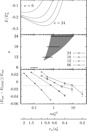
Figure 2: The lower panel shows the fractional difference of DMC interaction energy $E_{\text{DMC}}$ from the model $E_{\text{int}}$ with MFEG density $n$ (and Wigner-Seitz radius $r_{\text{s}}$) for different numbers of flavors, the dotted lines show $\pm 1\%$ disagreement. The central panel bars highlight the numerical region of applicability, the gray shaded area represents the analytically predicted region of $\pm 1\%$ applicability. The upper panel shows the total energy for 6, 12, 18 and 24 flavor electron gases.

The STLS results of Gold (1994) at $\nu=1$ were $\sim 3.4\%$ less negative than the DMC results of Ortiz and Ballone (1994), and at $\nu=6$ were $\sim 3.1\%$ less negative than our DMC results. This represents a significant difference between our and the STLS results when looking for the $1\%$ range of validity, highlighting the need for the more accurate DMC calculations. The range of validity at $\pm 1\,\%$ up to at least 24 flavors is to the high density side of the minimum in the total energy seen in Fig. 2, but the minimum $n_{\text{min}}\propto\nu^{8/5}$ lies within the region of validity for higher $\nu$. $n_{\text{min}}$ is the density expected to be seen in physical systems such as electron-hole drops, the good agreement of the theory with DMC results at this density indicates that the theory could be usefully applied to investigate the properties of physical systems, see for example Ref.Conduit (2008).

IV Static density-density response

Having verified the homogeneous system behavior we may now proceed and computationally examine inhomogeneous behavior through the static density-density (linear) response function Eqn. (3). The polarizability is an important quantity used Conduit (2008) to develop both homogeneous theory and the gradient correction, the density-density response function itself also governs the electrical response properties, for example polarization, screening, and behavior in an external potential; it is therefore useful to verify this response before applying the theory to model systems. We examine $1/\epsilon(\mathbf{q})$, the quantity probed experimentally Noziéres and Pines (1999).

DMC has previously been used to find the static density-density response of single-flavor systems: Sugiyama et al. (1992) applied the method to charged bosons, the density-density response of the electron gas was calculated by Moroni et al. (1992) (in two dimensions), and Bowen et al. (1994) and Moroni et al. (1995) (three dimensions). However, density-density response has not been studied numerically in a many-flavor system. Here we employ two methods to find the density-density response function. The more accurate and computationally efficient method of calculating the response is to examine the ground state energy, calculated using DMC. A VMC energy based estimate and an estimate using the induced electron density are used to check the accuracy of the trial wave function.

Before the results are described in Sec. IV.3, we outline the theory behind the two methods used to estimate the response, firstly in Sec. IV.1 by using the ground state energy variation, and secondly in Sec. IV.2 through the magnitude of the periodic density modulation.

IV.1 Ground state energy variation

To calculate the density-density response we use a weak probe so that the density response is solely due to the properties of the homogeneous system. We apply a static ($\omega=0$) monochromatic perturbative external potential $U(\mathbf{r})=U_{\mathbf{q}}\cos(\mathbf{q}\cdot\mathbf{r})$ to the homogeneous MFEG, corresponding to the background charge having an additional sinusoidal variation $n_{\text{ext}}(\mathbf{r})=n_{\mathbf{q}}\cos(\mathbf{q}\cdot\mathbf{r})$. The external potential and external charge are linked Sugiyama et al. (1992) through Poisson’s equation by

$$n_{\text{ext}}(\mathbf{k})=\frac{U_{\mathbf{q}}q^{2}}{8\pi}(\delta_{\mathbf{k},\mathbf{q}}+\delta_{\mathbf{k},\mathbf{-q}})\,.$$ (6)

We assume that different Fourier components are independent, the density response to an external potential with wave vector $\mathbf{q}$ and frequency $\omega$ is only at that wave vector and frequency so the induced charge is $n_{\text{ind}}(\mathbf{k})=\left(\left\langle\hat{n}_{\mathbf{k}}\right\rangle_{U_{\mathbf{q}}}-\left\langle\hat{n}_{\mathbf{k}}\right\rangle_{0}\right)(\delta_{\mathbf{k},\mathbf{q}}+\delta_{\mathbf{k},\mathbf{-q}})$. Here $\langle\hat{n}_{\mathbf{k}}\rangle_{U_{\mathbf{q}}}$ is the expectation value of the charge density Fourier component at wave vector $\mathbf{k}$ with an applied external potential $U_{\mathbf{q}}$, and $\langle\hat{n}_{\mathbf{k}}\rangle_{0}$ is the same but in the homogeneous case with no external potential. Linear response theory gives the static density-density response function as the ratio of the induced charge density and the perturbing external charge density so

$$\frac{1}{\epsilon(\mathbf{q})}=1+\frac{8\pi}{U_{\mathbf{q}}q^{2}}\left(\left\langle\hat{n}_{\mathbf{q}}\right\rangle_{U_{\mathbf{q}}}-\left\langle\hat{n}_{\mathbf{q}}\right\rangle_{0}\right)\,.$$ (7)

If the external potential is small relative to other typical energies the density response is determined solely by the properties of the homogeneous MFEG. We can expand in small $U_{\mathbf{q}}$ so that

$$\left\langle\hat{n}_{\mathbf{k}}\right\rangle_{U_{\mathbf{q}}}-\left\langle\hat{n}_{\mathbf{k}}\right\rangle_{0} \approx \left.U_{\mathbf{q}}\frac{\text{d}\left\langle\hat{n}_{\mathbf{k}}\right\rangle}{\text{d}U_{\mathbf{q}}}\right|_{U_{\mathbf{q}}=0}=\left.U_{\mathbf{q}}\frac{\text{d}^{2}E}{\text{d}U_{\mathbf{q}}^{2}}\right|_{U_{\mathbf{q}}=0}\,,$$ (8)

where the induced charge density is calculated by considering the dependence of the ground state energy $E$ on the magnitude of the external field. Substituting this into Eqn. (7) gives an expression for the density-density response

$$\frac{1}{\epsilon(\mathbf{q})}=1+\frac{8\pi}{q^{2}}\left.\frac{\text{d}^{2}E}{\text{d}U_{\mathbf{q}}^{2}}\right|_{U_{\mathbf{q}}=0}\,.$$ (9)

To recover the density-density response function at a particular wave vector, several QMC calculations were performed at that wave vector for different amplitudes of the external field. A polynomial fit was made to the ground state energy so as to extract the second derivative. To investigate the lowest order polarizability the applied external field should be as small as possible yet still give statistically significant results, to ensure this we checked that the ground state energy showed only quadratic behavior with applied field amplitude. A further convenient way to check the perturbing field is sufficiently small is to ensure the electric field of the external potential is less than the typical electric field strength between two neighboring electrons, $e/r_{\text{s}}^{2}$.

IV.2 Induced charge density measurement

As the external potential is perturbative we use the same plane-wave basis set as employed for the calculations on the homogeneous MFEG described in Sec. III. To account for the modulating density, following Moroni et al. (1992), Bowen et al. (1994), and Moroni et al. (1995) we introduce a new $q$ term into the Jastrow factor of the form

$$q(\mathbf{r}_{i})=b\cos(\mathbf{q}\cdot\mathbf{r}_{i})\,,$$ (10)

where $b$ is an optimizable parameter, $\mathbf{r}_{i}$ the position of the $i$th electron, and the wave vector $\mathbf{q}$ corresponds to that of the perturbative external potential. As $b$ is small, the charge density induced by the perturbative external potential is $n_{\text{ind}}\approx 2b\cos(\mathbf{q}\cdot\mathbf{r}_{i})$. From Eqn. (6) and Eqn. (7) it follows that

$$\frac{1}{\epsilon(\mathbf{q})}=1+\frac{8\pi b}{q^{2}U_{\mathbf{q}}}\,.$$ (11)

The optimized value of $b$ was found by variance minimization during a VMC calculation. The relationship then allows us to derive an estimate for the density-density response function for each separate $U_{\mathbf{q}}$, typically four values were averaged to give a final estimate for the density-density response.

IV.3 Results

We chose to find the polarizability for a MFEG with $\nu=24$ and $r_{\text{s}}=0.6a_{0}^{*}$. This lies at the lower bound of the range of validity near to the minimum in the energy (see Fig. 2) at a density expected to be seen in physical systems. This density was also chosen since it had most of the polarizability curve $0.25<1/\epsilon\leq 1$ in the region of applicability $q\geq 2p_{\text{F}}$. Boundary conditions mean that the external potential must be periodic over the simulation cell, therefore the external potential wave vector $\mathbf{q}$ must be a reciprocal lattice vector. We checked that if the Jastrow factor $q$ term wave vector was changed so that it was incommensurate with the external potential then following optimization $b=0$ within statistical errors; this verified the linear response assumption that Fourier components are independent.

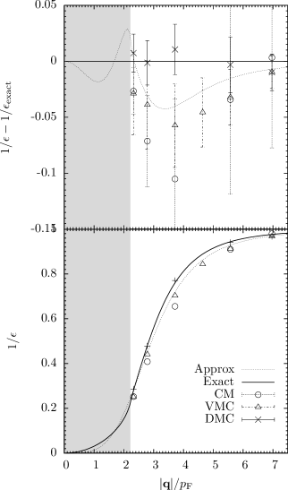
Figure 3: The density-density response $1/\epsilon$ versus the wave vector $|\mathbf{q}|$ of a MFEG with $\nu=24$ and $r_{\text{s}}=0.6a_{0}^{*}$. The solid curve shows the exact result $1/\epsilon_{\text{exact}}$ (Eqn. (2)), the dotted curve the Eqn. (3) approximation. The shaded grey region $|\mathbf{q}|/2<p_{\text{F}}$ is where the many-flavor limit breaks down. The points show the values for the permittivity calculated from QMC results, the circle is from modulated charge measurements (CM), the triangle from VMC energy and the cross from DMC energy. The lower panel plots the actual response, the upper panel shows the deviation of response from the exact theoretical result Eqn. (2) with standard error bars.

The results of the calculation are shown in Fig. 3. The DMC results obtained by considering the variation in ground state energy (see Sec. IV.1) better fits the exact than approximate expression for the polarizability, and though error bars are large can distinguish between the two within one standard deviation. This shows that QMC results can exceed the accuracy of the approximation made in Eqn. (3), though that estimate remains useful. The positive agreement verifies the theory and confirms the accuracy of the CASINO simulations.

The ground state energies calculated by VMC were used in the same way as the DMC results to find the density response and provide a reasonable fit, though here error bars are large so comparison is difficult. Following the prescription in Sec. IV.2 we also derived values for the density-density response function using the charge density modulation at the wavelength of the perturbing potential, $U_{\mathbf{q}}$. These values agreed within statistics though carried a larger uncertainty than those derived using the ground state energy. Both of these alternative methods appear to underestimate the density-density response. These results are consistent, a smaller charge density response gives a smaller coefficient in the Jastrow factor $q$ term and a smaller reduction in ground state energy. Nevertheless, the reasonable agreement of both VMC estimates and to the DMC results indicates that the trial wave function had an adequate nodal surface.

V Gradient correction

It was important to verify the density-density response as it is a key component to the many-flavor formalism and could be applied to other many-flavor systems where density is expected to be inhomogeneous, for example junctions and the response to defects and impurities. Now that it has been verified, we may proceed to consider a quantity derived from it: the gradient expansion, Eqn. (5), which is also useful for analyzing systems with inhomogeneous density. Once we have investigated the validity of such an expansion we can apply the formalism to quantum dots, chosen since they have a large controllable variation in electron density so should provide a good test of the gradient expansion. Quantum dots are commonly made in many-flavor semiconductor materials so can be modeled using a many-flavor formalism, and are a system in which there is current research interest.

Quantum dots Bányai and Koch (1993); Reimann and Manninen (2002) have not previously been studied in the many-flavor limit though there have been several previous computational studies of a single-flavor electron gas confined in a quantum dot. Previous QMC simulations of quantum dots include Pollock and Koch (1991), Harju et al. (1999) performed VMC calculations for parabolically confined electrons in circular dots. Bolton (1996) performed fixed-phase DMC simulations. Path-integral QMC calculations have also been performed Lozovik and Mandelshtam (1992); Mak et al. (1998); Egger et al. (1999), these showed poor agreement with results from exact diagonalization Eto (1997). Benedict et al. (2003); Williamson et al. (2002); Puzder et al. (2003) all compared the optical band-gap between DMC calculations and results from other methods. For circular quantum dots Pederiva et al. (2000) found the ground-state using both DMC, a local spin density approximation method, and Hartree-Fock, they then directly compared the ground-state energy, correlation energy, and spin density profiles. Ghosal et al. (2006) also used DMC to investigate circular quantum dots. Quantum dots have successfully been investigated using DFT Ferconi and Vignale (1994); Koskinen et al. (1997); Hirose and Wingreen (1999); Pederiva et al. (2000), Pederiva et al. (2000) found the local spin density approximation method predicted ground-state energies that were typically $2\,\%$ greater than DMC energies, Ferconi and Vignale (1994) obtained a $3\,\%$ agreement between current-density-functional theory and exact diagonalization results.

V.1 Method

Before describing the study of quantum dots using a many-flavor functional in detail we first outline the general strategy of the numerical calculations. Firstly, a DFT calculation using the many-flavor functional (including the gradient approximation) was performed using a plane-wave basis set. This produced an estimate of the ground-state energy and density according to the many-flavor theory. It also provided a trial wave function that was converted to a B-spline basis set and, with Jastrow factor, was optimized in a VMC calculation, in preparation for a DMC calculation. Finally, the DMC calculation gave a second estimate of the ground state energy and density, exact only for the fixed node approximation. This estimate was compared with the DFT calculation, and also gave an insight into the accuracy of the many-flavor theory.

Here we carried out simulations on a quantum dot with a harmonic external potential of the form $V=kr^{2}/2$, where $r$ is the distance to the center of the quantum dot containing a MFEG with 12 flavors. This potential was chosen as it is simple, continuous, realistic Tarucha et al. (1996); Sasaki et al. (1998), and has been used in previous computational studies Ferconi and Vignale (1994); Ashoori (1996); Koskinen et al. (1997); Kouwenhoven et al. (1997); Harju et al. (1999); Hirose and Wingreen (1999); Pederiva et al. (2000); Reusch (2003). Filled shells in this potential correspond to $1,4,10,20,35,\dots$ orbitals (whose degeneracy may be reduced by electron-electron interactions). In DFT we used a supercell containing a single dot to model the aperiodic system with periodic boundary conditions, in DMC non-periodic calculations with just a single quantum dot were performed. The cubic cell was large enough that the trial wave functions had reduced by at least a factor of $10^{-4}$ at its boundary.

Trial wave functions were generated using the DFT program 3Ddotdft, an extended version of DOTDFT Hine . This used the many-flavor functional with gradient approximation so had energy density

$$\varepsilon(n(\mathbf{r}))=-A_{3\text{D}}n^{5/4}+\xi\frac{|\nabla n|^{2}}{8n}\,.$$ (12)

A new parameter $\xi$ was introduced that multiplies the gradient term, which allowed us to adjust its size; $\xi=1$ gives the correct analytical expression, and $\xi=0$ the functional without a gradient expansion.

The VMC simulations, run in CASINO, used a B-spline basis set Hernández et al. (1997); Alfè and Gillan (2004) because a localized basis set offers significant performance advantages over plane-waves. The wave function was optimized in VMC with a Jastrow factor containing the two-body polynomial $u$ term and two-body plane-wave term $p$ with the same form as used in Sec. III and Sec. IV, and a one-body electron-potential term $\chi(r_{i})=F(r_{i})\sum_{m=2}^{6}\beta_{m}r_{i}^{m}$ with $F$ determining behavior at the cutoff length, $r_{i}$ the distance of the $i$th electron from the center of the potential, and the $\beta_{m}$ being optimizable parameters; we also note that the $\chi$ term has no central cusp.

The many-flavor functional incorrectly adds in the self-interaction energy of each electron to its own Coulomb potential. One way to correct for this is to add an additional term to the density functional Perdew and Zunger (1981); Dreizler and Gross (2001). However, as the number of flavors is increased the ratio of the correct interaction ($\propto\nu^{2}$) to incorrect self-interaction ($\propto\nu$) increases as $\sim 2\nu-1$ so in the many-flavor limit the self-interacting energy error may be neglected. To ensure the B-spline grid was sufficiently fine, we compared the trial wave function kinetic and external potential energy before and after conversion the B-spline basis set. We also checked the choice of DMC time-step was sufficiently small, the number of configurations was suitably large, and the simulation cell size was adequately large. On changing these variables the variation in the ground state energy was $\Delta E\approx 0.02E_{\text{h}}^{*}$, sufficiently small to allow us to compare the ground state energy as the potential strength and gradient expansion coefficient were varied.

V.2 Results

We analyzed a quantum dot containing a MFEG of 12 flavors and 4 bands (shells), containing a total of 96 electrons. This was chosen since it had a full shell so is expected to have a zero spin ground-state Reimann and Manninen (2002) that can be analyzed with the many-flavor functional, was computationally feasible, and contained enough electrons to be in the LDA regime, where the many-flavor functional is expected to apply.

Two different investigations were carried out to probe effects of changing the density gradient, firstly strength of the dot confining potential $k$ was changed, and secondly the gradient expansion coefficient $\xi$ was varied.

V.2.1 Varying the external potential strength $k$

Figure 4: In the upper plot the crosses and solid line show the difference between DFT $(E_{\text{DFT}})$ and DMC $(E)$ energies with varying external potential strength $k$, if agreement were exact, points would lie along the horizontal dotted line. In the lower plot the circles and solid line show the maximum density gradient of the dots with varying $k$, and the squares and dashed line the gradient at which the theory breaks down.

At the strong external potential $k=8$, corresponding to steep gradients, Fig. 4 shows the DFT energy is overestimated compared with the DMC result, indicating that the gradient approximation is not applicable and that the next order term in a gradient expansion is negative. Fig. 5 shows that the DFT density profile underestimates the true density towards the center of the dot and overestimates density in the outer regions, indicating that the DFT functional does not favor steep enough gradients. This is consistent with the next term in the gradient expansion being negative. The breakdown corresponds to a coefficient of $\alpha\approx 1.8$ in $q_{\text{max}}=\alpha(\hbar a_{0}^{*-1/4})n^{1/4}$, close to the $\alpha\approx 4$ which corresponds to the maximum contribution to the interacting energy.

At the intermediate potential $k=1$ the DFT and DMC estimates of energy and the density profile agree, in this region the gradient approximation applies. The DFT density profile shows a slight over-density at the center, consistent with self-interaction energy being included in the DFT calculation. At the weak potential $k=0.1$ electron densities are low meaning the homogeneous interacting energy is outside of its region of applicability (see Fig. 2), therefore the DFT energy is an overestimate.

Figure 5: The lower panel shows the density profile of quantum dots estimated using both DFT and DMC at external potential strengths of $k=1$ and $k=8$. The difference between the DFT and DMC results at $k=1$ and $k=8$ is shown in the upper panel. The DMC statistical error is less than the size of the points.

V.2.2 Varying the gradient term coefficient $\xi$

Figure 6: The upper panel shows, for dots with external potential strength $k=1$, the density profile maximum gradient as a function of $\xi$. The central panel shows the variation of external potential DFT energy based on the primary $y$-axis using square points and the solid line, the secondary $y$-axis shows electron-electron DFT energy using crosses and the dashed line. The lower panel solid line shows the variation of DFT ground state energy with $\xi$, and the horizontal dotted line the ground-state energy predicted using DMC from the $\xi=1$ trial wave function. The DMC statistical error is less than the size of the points.

Fig. 6 shows results of simulations on dots, chosen to have a potential strength $k=1$, which is at the center of agreement of the previous results. The best agreement between the DFT and DMC ground state energy is at $\xi\sim 0.9$. This is in good agreement with the expected $\xi=1$, the difference may be due to systematic errors such as the self-interacting energy or higher order gradient terms. As expected, the energy is overestimated for dots with too large a gradient expansion term, and underestimated for dots with too small a gradient correction term.

The maximum gradient seen in the dot density profile decreases as $\xi$ increases (see Fig. 6). The dot becomes more spread out so the external energy $E_{\text{ext}}$ increases whilst the total electron-electron Coulomb energy $E_{\text{e-e}}$ decreases. Overall the total DFT energy increases. Three quantum dot electron density profiles for gradient term coefficients $\xi=1$, 2, and 3 are shown in Fig. 7. Compared with the dot calculated with $\xi=1$, the dot generated with no energy penalty for gradients, $\xi=0$, has a high central and low outer density showing that it has a higher gradient in the density. Conversely dot with increased energy cost for gradients, $\xi=2$, has a more shallow profile.

Figure 7: The upper panel shows the variation of the $\xi=0$ (dotted line, squares) and the $\xi=2$ (dashed line, crosses) DFT density profiles from the $\xi=1$ DFT density profile. The lower panel shows DFT density profiles for $\xi=0$, $\xi=1$ (solid line, triangles), and $\xi=2$ in a $k=1$ dot.

The density profiles seen in Fig. 5 and Fig. 7 can be further analyzed in light of other theoretical studies of quantum dots reviewed in Ref. Reimann and Manninen (2002). The density profile calculated using the many-flavor functional is not flat at the center, but instead has correlation-induced density inhomogeneity evidenced by a characteristic minimum in the density at $r\approx 2a_{0}^{*}$. The intermediate density regime in which this occurs is consistent with the strong correlations causing a minimum in the total many-flavor energy density Conduit (2008). It is also akin to the intermediate density regime seen in other quantum dot systems Egger et al. (1999); Reimann and Manninen (2002); Ghosal et al. (2006); Kalliakos et al. (2008), in the high density limit the quantum dot has properties like a Fermi liquid with de-localized electrons Egger et al. (1999); Reimann and Manninen (2002); Giuliani and Vignale (2005), whereas in the low density limit the electrons become crystalline Lozovik and Mandelshtam (1990, 1992); Bolton and Rössler (1993); Date et al. (1998); Egger et al. (1999); Reimann and Manninen (2002) inside the dot. As the many-flavor functional was successful in predicting correlation-induced inhomogeneities, it could be used to investigate other many-flavor quantum dot effects including the Kondo effect in multi-valley semiconductors Shiau et al. (2007); Shiau and Joynt (2007), the reduction of valley degeneracy of coupled quantum dots Hada and Eto (2003); Ahn (2005); Belyakov and Burdov (2007), and harmonically trapped cold atoms with an additional quantum number denoting energy level Honerkamp and Hofstetter (2004a, b); Cherng et al. (2007); Yannouleas and Landman (2007).

VI Conclusions

We have computationally verified the theory of the MFEG presented in Conduit (2008) using QMC simulations. In a homogeneous system, DMC estimates for the ground state energy are consistent with theory and the theoretically estimated density range over which the theory applies is consistent with numerical results. The applicable density for $\text{Bi}_{2}\text{Te}_{3}$ $(\nu=6)$ corresponds to a charge carrier density between $7\times 10^{19}\,\text{cm}^{-3}$ and $2\times 10^{20}\,\text{cm}^{-3}$.

The density response function for a MFEG with 24 flavors was found using three methods: density modulation predicted by VMC, and the variation in ground state energy predicted by VMC and also by DMC. The two VMC results underestimated the response $1/\epsilon$, but the DMC results agreed with theory and could distinguish between the exact and a useful approximate expression for polarizability.

We used a many-flavor functional including a local gradient approximation in DFT calculations of large quantum dots. The DFT calculation estimated the ground-state energy and wave function, which were verified by a DMC calculation. We found the high gradient breakdown of the expansion was at $q_{\text{max}}\approx 1.8(\hbar a_{0}^{*-1/4})n^{1/4}$, the low gradient breakdown was consistent with the homogeneous MFEG lowest applicable density, and that the gradient expansion was applicable in the intermediate regime. The many-flavor functional, used as part of DFT calculations, could be a useful tool for analyzing other multi-valley semiconductor systems.