Multi-Avalanche Correlations in Directed Sandpile Models

Abstract

Multiple avalanches, initiated by simultaneously toppling neighbouring sites, are studied in three different directed sandpile models. It is argued that, while the single avalanche exponents are different for the three models, a suitably defined two-avalanche distribution has identical exponents. The origin of this universality is traced to particle conservation.

The sandpile model is a paradigm for self-organized criticality wherein long range correlations are generated without any parameter being fine tuned Bak et al. (1987, 1988). The original version of the model and its variants (see Dhar (2006) for a review) have a common feature: slow driving during which particles are added to the system, and fast dissipation during which the system relaxes through avalanches. The steady state is characterized by power law correlations.

Conservation laws are known to constrain correlation functions of driven–dissipative systems. A well known example is the Kolmogorov $4/5$-th law of three dimensional fluid turbulence Kolmogorov (1941, 1942); Falkovich (2004); Frisch (1995). The conserved quantity is energy which is pumped in at large length scales and dissipated through viscosity at small length scales. The $4/5$-th law states that, in the inertial range [distances $r$ between driving and dissipation length scales], $\langle[v_{l}(\vec{r},t)-v_{l}(\vec{0},t)]^{3}\rangle=-\frac{4}{5}\epsilon r$, where $v_{l}(\vec{r},t)$ is the longitudinal component of the velocity at point $\vec{r}$ at time $t$, and $\epsilon$ is the energy dissipation rate. The linear dependence on $r$ remains true in all dimensions, while the proportionality constant is a function of dimension. There are other examples, mainly from turbulence, of a correlation function being determined by the constant flux of a conserved quantity. Examples include magneto-hydrodynamics Gomez et al. (2000), burgers turbulence Falkovich (2004) and advection of a passive scalar (see Falkovich et al. (2001) and references within). These relations are central to understanding turbulence, acting as checkpoints for phenomological theories. Examples outside turbulence are few. In a recent paper Connaughton et al. (2007a), this relation was generalised to an arbitrary driven dissipative system that showed the general features of turbulence. Exact results were obtained for specific models, namely wave turbulence Zakharov et al. (1992) and models of diffusing–aggregating particles Connaughton et al. (2008); Connaughton et al. (2007b).

In sandpile models, the total number of particles is conserved in each toppling. As a consequence, can any correlation function be determined? In this paper, we answer this question in the context of directed sandpile models. Consider multiple avalanches obtained by adding particles simultaneously at nearby lattice sites. It is argued that a suitably defined two avalanche joint probability distribution function [defined later] will play the role of the three point velocity correlations in the Kolmogorov $4/5$-th law, and will have a scaling exponent which is independent of dimension and hence identical to the mean field answer.

We define the three sandpile models studied in this paper on a directed square lattice of horizontal extent $L$ and vertical extent $T$ (see Fig. 1). Periodic boundary conditions are imposed in the $x$-direction and open boundary conditions along the $t$-direction, also referred to as the time direction. The number of particles at a site $(x,t)$ is denoted by a non-negative integer $h(x,t)$. All the three models are driven by adding a particle to a randomly chosen site on the top layer ($t=0$) and then letting the system relax according to the following rules of evolution.
The deterministic model Dhar and Ramaswamy (1989): A stable configuration has all $h(x,t)=0,1$. If $(h,x,t)\geq 2$, then it relaxes by transferring two particles, one each to its two downward neighbours, i.e, $h(x,t)$ decreases by $2$ and $h(x-1,t+1)$ and $h(x+1,t+1)$ increase by one.
The stochastic model Paczuski and Bassler (2000); Kloster et al. (2001): This model has the same rules of evolution as the deterministic model except for one difference. The toppling is now stochastic. When a site $(x,t)$ topples, with probability $1/4$ both particles go to $(x-1,t+1)$, with probability $1/4$ both particles go to $(x+1,t+1)$, with probability $1/2$, $(x-1,t+1)$ and $(x+1,t+1)$ receive one particle each.
The sticky model Tadić and Dhar (1997): In this model, the heights can take any non-negative integer value. A site is considered unstable if $h(x,t)\geq 2$ and it received at least one particle the previous time step. All unstable sites relax simultaneously as follows: With probability $p$, the height decreases by $2$ and a particle is added to each of its downward neighbours. With probability $(1-p)$, the site becomes stable without losing any particles.

Figure 1: The directed square lattice with $L$ sites along the $x$-axis and $T$ sites along the $t$-axis. Periodic boundary conditions are applied in the horizontal direction.

In all the three models, if a site at the bottom ($t=T$) topples, then the height at that site reduces by two, and the two particles are removed from the system. An avalanche is defined as the number of topplings that the system undergoes after a particle is added to a stable configuration. In the steady state, the probability of an avalanche of size $s$ is a power law distribution $P(s,T)\sim s^{-\tau}f(sT^{-\delta})$, when $L\gg T^{1/z}$, where $z$ is the dynamic exponent. These two exponents are not independent from each other. Particle conservation from layer to layer results in the scaling relation $\langle s\rangle\sim T$ (for example, see Dhar (2006)), implying that $\delta(2-\tau)=1$.

The three models belong to three different universality classes. For the deterministic model, first studied in Ref. Dhar and Ramaswamy (1989), $\tau=4/3$, $\delta=3/2$ in $d=2$, $\tau=3/2$, $\delta=2$ in $d>3$. In $d=3$, the mean field results have logarithmic corrections Dhar and Ramaswamy (1989). Stochasticity in the toppling rules is known to change the universality class of sandpile models Manna (1991). For the stochastic model, it was argued that $\tau=10/7$, $\delta=7/4$ in $d=2$, $\tau=3/2$, $\delta=2$ in $d>3$, with $d=3$ having the mean field exponents with logarithmic corrections Paczuski and Bassler (2000); Kloster et al. (2001). The sticky model was introduced in Ref. Tadić and Dhar (1997). Introducing stickiness changes the universality class of the sandpile model away from deterministic and stochastic classes Mohanty and Dhar (2002). The avalanche exponents are then related to the exponents of directed percolation. From the best numerical estimates for directed percolation exponents, it was shown that $\tau\approx 1.32$, $\delta=1.47$ in $d=2$ Tadić and Dhar (1997). In addition to having different exponents, the sticky model is not abelian, unlike the other two models.

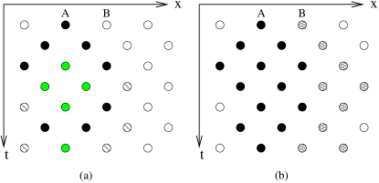
Figure 2: (a) The avalanche when site $A$ is toppled is shown by filled circles (black or grey). The black circles have height $0$ after the avalanche. The grey circles have the same height as before the avalanche. The circles with diameter drawn are not part of the avalanche, but will have height $1$ after the avalanche. (b) The avalanche when $B$ is toppled after $A$ is shown by hatched circles. The left boundary of the avalanche $B$ is adjacent to the right boundary of avalanche $A$.

We now define the two-avalanche distributions. Consider avalanches initiated by adding two particles simultaneously at nearby lattice sites (denoted by 1 and 2) on the top level. Let the set of sites belonging to the avalanche associated with site 1 (site 2) be denoted by $S_{1}$ ($S_{2})$. When a site topples, if it had received particles from only sites in $S_{1}$ ($S_{2})$, then the site is assigned to $S_{1}$ ($S_{2})$. If on the other hand, it had received particles from sites belonging to $S_{1}$ as well as $S_{2}$, then the site is assigned randomly to one of the sets. Let $s_{1}$ ($s_{2}$) denote the number of topplings undergone by sites in $S_{1}$ ($S_{2})$. We will denote the joint probability distribution by $P_{1}(s_{1},s_{2})$. For abelian models, we can also define a two avalanche distribution as follows. Topple a site. Let the avalanche size be $s_{1}$. Then topple the neighbouring site. Let the avalanche distribution be $s_{2}$. Let the joint probability distribution be denoted by $P_{2}(s_{1},s_{2})$. In this paper, it is argued that $P_{1}$ and $P_{2}$ have scaling exponents $3$ in all dimensions, i.e.,

$$P_{i}(\Lambda s_{1},\Lambda s_{2})=\frac{1}{\Lambda^{3}}P_{i}(s_{1},s_{2}),\quad i=1,2.$$ (1)

We give a heuristic argument supporting this conjecture. Consider the single avalanche probability $P(s,t)$. In continuous time, it schematically obeys the equation

$$\frac{dP(s,t)}{dt}\sim\int ds_{1}ds_{2}P_{1}(s_{1},s_{2})\delta(s_{1}+s_{2}-s),$$ (2)

where $P_{1}$ is the two avalanche distribution defined above. Use the fact that, for all the three models $\langle s\rangle\simeq Jt$, where $J$ is a constant Dhar (2006). Multiply Eq. (2) by $s$ and integrate over $s$. The left hand side is a constant independent of $t$ and $s$. Equation (2) then reduces to

$${\rm const}\sim\int dsds_{1}ds_{2}sP_{1}(s_{1},s_{2})\delta(s_{1}+s_{2}-s).$$ (3)

A dimensional analysis of the right hand side of Eq. (3) immediately predicts

$$P_{1}(s,s)\sim\frac{1}{s^{3}},$$ (4)

or more generally Eq. (1) with $i=1$. For the abelian versions of the model, the order of toppling is not crucial. Hence, one can conjecture that instead of simultaneous toppling, the toppling could be sequential and that $P_{2}$ obeys the same scaling law as in Eq (1).

We now give a direct proof that, in the deterministic model, $P_{2}(s_{1},s_{2})$ has the scaling as in Eq. (1). In the steady state, each configuration of the model has equal weight Dhar and Ramaswamy (1989). Thus, each height is $0$ and $1$ with probability $1/2$ independent of other sites. The avalanches then have no holes i.e., an avalanche is described by the two boundaries, each of which are random walkers that annihilate on contact. The clusters also have the following property. Consider the right boundary. If it is at $(x,t)$, the next time step, it can either go to $(x+1,t+1)$ or $(x-1,t+1)$. If it goes to $(x+1,t+1)$, then $h(x,t)=0$. It it goes to $(x-1,t+1)$, then $h(x+1,t+1)=1$. Similar rules exist for the left walker. An example is shown in Fig. 2(a) with site $A$ having been toppled. Now consider the case when $B$ (see Fig. 2(b)) is toppled. The black circles cannot topple because they have height $0$, ensuring that the two avalanches do not overlap. On the other hand, the sites with height $1$ will necessarily topple provided the avalanche survives up to that level. Hence the right boundary of first avalanche and the left boundary of second avalanche will be adjacent to each other (see Fig. 2(b)).

The calculation of $P_{2}(s_{1},s_{2})$ now reduces to the problem of three annihilating walkers. Let us calculate the probability that both avalanches exceed time $t$. This is equal to the survival probability of three annihilating random walkers up to time $t$, which varies as $t^{-3/2}$ when $t\gg 1$ Fisher and Gelfand (1988). Using the scaling $s\sim t^{3/2}$ Dhar and Ramaswamy (1989), we obtain that $\int_{s}^{\infty}\int_{s}^{\infty}ds_{1}ds_{2}P_{2}(s_{1},s_{2})\sim s^{-1}$, or $P_{2}(s,s)\sim s^{-3}$, consistent with Eq. (1). The argument for $P_{1}(s_{1},s_{2})$ proceeds on exactly the same lines and we omit the argument here.

Figure 3: The variation of (a)$P_{1}(s,s_{1})$ and (b) $P_{2}(s,s_{1})$ with $s$ is shown for the deterministic model for $s_{1}=s,s\sqrt{2},s$. The bottom two curves have been shifted for clarity. The solid lines are power laws with exponent (a) $2.97$ and (b) $2.98$.

Figure 4: The variation of (a)$P_{1}(s,s_{1})$ and (b) $P_{2}(s,s_{1})$ with $s$ is shown for the stochastic model for $s_{1}=s,s\sqrt{2},s$. The bottom two curves have been shifted for clarity. The solid lines are power laws with exponent (a) $3.03$ and (b) $3.00$.

Figure 5: The variation of $P_{1}(s,s_{1})$ with $s$ is shown for the sticky model for $s_{1}=s,s\sqrt{2},s$. The simulations are for $p=0.85$. The bottom two curves have been shifted for clarity. The solid lines are power laws with exponent $3.03$.

For the other two models, we rely on Monte Carlo simulations. Simulations were done for a lattice with $L=1024$ and $T=8192$. Logarithmic binning was used with bin size $\ln(\sqrt{2})$. In the steady state, the data was averaged over $2\times 10^{8}$ avalanches initiated by toppling nearest neighbours. These multi avalanches were interspersed with single site avalanches. Avalanches that reached the boundary were omitted from the statistics in order to prevent strong finite size corrections Tebaldi et al. (1999).

We study the variation with $s$ of the probability distributions $P_{1}(s,s_{1})$ and $P_{2}(s,s_{1})$ with $s_{1}=s,s\sqrt{2},2s$. The exponents are determined through the maximum likelihood estimator method Goldstein et al. (2004); Newman (2005). Let $P_{i}(s_{1},s)\sim(s_{1}s)^{-\tau_{i}/2}$, for $i=1,2$. The numerical estimates for $\tau_{1}$ and $\tau_{2}$ are shown in Table 1. The data is shown in Figs. 3 [deterministic],4 [stochastic], and 5 [sticky], all in good agreement with Eq. (1).

Table 1: Numerically obtained values for the exponents $\tau_{1}$ and $\tau_{2}$ for the different models.

Model	$\tau_{1}$	$\tau_{2}$
Deterministic	$2.97\pm 0.04$	$2.98\pm 0.04$
Stochastic	$3.03\pm 0.05$	$3.00\pm 0.04$
Sticky	$3.03\pm 0.06$	-

In dimensions greater than the upper critical dimension, we expect the scaling in Eq. (1) to hold, the meanfield avalanche exponent being $3/2$. The deviation from meanfield should be most pronounced in two dimensions for which Eq. (1) has been numerically verified. In other dimensions, we expect that an equation of the form Eq. (2) should hold, maybe with a different joint probability distribution. For example, in three dimensions, it will be $P_{1}(s_{1},s_{2},s_{3})$. However, the main contribution to this three point function will be when one of the $s_{i}$’s is small and we retrieve an effective two-point function.

To summarize, the two-avalanche distribution was studied for three directed sandpile models. While the three models have different exponents for the single site avalanche distribution, it was shown numerically and through a heuristic argument that the two avalanche distribution is the same for all three. Exact results were obtained for the deterministic model. The robustness of the result is due to particle conservation layer by layer, leading to the scaling relation $\langle s\rangle\sim t$, and is not dependent on the details of the model.