STATIONARY PRECESSION TOPOLOGICAL SOLITONS WITH NONZERO HOPF INVARIANT IN A UNIAXIAL FERROMAGNET

Abstract

Three-dimensional stationary precession solitons with nonzero Hopf indices are found numerically by solving the Landau Lifshitz equation. The structure and existence domain of the solitons are found.

Topological three-dimensional solitons attract considerable interest in many fields of physics including hydrodynamics, particle physics, cosmology, and condensed matter physics. In models with the three-component unit vector field ${\bf n}=(n_{1},n_{2},n_{3})$, where ${\bf n}^{2}=1$, localized structures exist if the field $n$ asymptotically approaches the vector ${\bf n}_{0}$ as $|{\bf r}|\to\infty$. Such fields map the $R^{3}\cup\{\infty\}$ space to the two-dimensional sphere $S^{2}$ and are classified by the homotopy classes $\pi_{3}(S^{2})=Z$ and characterized by the Hopf invariant  bib:BW given by the expression:

$$H=-\frac{1}{(8\pi)^{2}}\int{\bf F}\cdot{\bf A}d{\bf r},$$ (1)

where $F_{i}=\epsilon_{ijk}{\bf n}\cdot(\bigtriangledown_{j}{\bf n}\times\bigtriangledown_{k}{\bf n})$ and $curl{\bf A}=2{\bf F}$. The invariant $H$ admits the simple geometric interpretation as the linking number of two preimage closed curves corresponding to an arbitrary pair of points on the $S^{2}$ sphere.

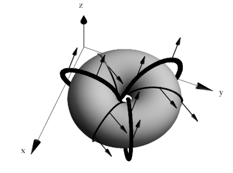
Figure 1: Distribution of magnetization in a three-dimensional topological soliton with $H=3$. The thin and thick curves are the preimages of the points $(\Theta_{1},\Phi_{1})=(0.5\pi,1)$ and $(\Theta_{2},\Phi_{2})=(0.2\pi,3)$ on the $S^{2}$ sphere, respectively.

Stable three-dimensional solitons with $H\neq 0$ (the so-called knotted solitons) were studied numerically in the Faddeev-Niemi model bib:LD ; bib:LN ; bib:LN1 ; bib:BS ; bib:Glad , i.e., the nonlinear $\sigma$-model including terms with fourth-order derivatives. Defects with a nonzero Hopf invariant have been discussed in condensed matter physics since the pioneering works by Volovik and Mineev for superfluid ${}^{3}He$ bib:VM and by Dzyaloshinskii and Ivanov bib:DI for a uniaxial ferromagnet. Simple reasoning based on the Derrick theorem bib:Derrick indicates the absence of nontrivial static threedimensional solitons with finite energy in the aforementioned media. However, dynamical structures of this kind, which are stabilized by the precession of the magnetization, can exist bib:KBK ; bib:PT . Studies of threedimensional magnetic structures are of both academic and engineering interest in view of the development of new memory elements based on topological solitons in uniaxial ferromagnets bib:OBS .

Three-dimensional magnetic structures have been poorly studied until recently. A few original theoretical and experimental works on magnetic structures in superfluid ${}^{3}He$ were published in recent years bib:Volovik1 ; bib:Volovik2 ; bib:Volovik3 ; bib:Volovik4 . Spiral and cnoidal hedgehogs with $H=0$ were analytically described in  bib:Borisov in the Heisenberg model for an isotropic ferromagnet. Constant-velocity precession solitons with $H=1$ were numerically found in the same model bib:Cooper . Both stationary (magnon drops)  bib:IvKos1 and uniformly moving bib:Sut2001 precession radially symmetric nontopological solitons in a uniaxial ferromagnet were analyzed. In addition, the moving topological soliton was recently analyzed bib:Sut2007 , but stable configurations with $H\neq 0$ were not found.

In this work, we find dynamical structures, namely, stationary precession three-dimensional solitons with nonzero Hopf indices, in a uniaxial ferromagnet. Hereafter, the existence domain of such solitons is determined and their fine structure and main features are studied.

The dynamics of the magnetization vector is described by the Landau-Lifshitz equation. In the case of negligible relaxation, this equation has the form

$$\frac{\partial{\bf M}}{\partial t}=-\frac{2\mu_{0}}{\hbar}\left[\frac{\delta{E}}{\delta{\bf M}}\times{\bf M}\right],$$ (2)

where the ferromagnet energy $E=E_{exch.}+E_{anis.}$ is the sum of the exchange energy $E_{exch.}$ and the magnetic anisotropy energy $E_{anis.}$ with the parameter $\beta$:

$$E_{exch.} =\frac{\alpha}{2}\int\left(\frac{\partial{\bf M}}{\partial{r_{i}}}\right)^{2}d{\bf r},$$ (3)

$$E_{anis.} =\frac{\beta}{2}\int\left({M_{x}}^{2}+{M_{y}}^{2}\right)d{\bf r}.$$ (4)

The energy of the magnetic-dipole interaction is negligible for large $\beta$ values typical for many magnetic media.

Using the parameterization

$$\begin{cases}{\bf M}=M_{0}{\bf n},\\ {\bf n}=(sin\Theta cos\Phi,sin\Theta sin\Phi,cos\Theta),\end{cases}$$ (5)

we seek solutions describing stationary precession solitons of the form

$$\begin{cases}\Phi=\omega t+Q\varphi+\phi(r,z),\\ \Theta=\theta(r,z),\end{cases}$$ (6)

where $\varphi$ is the polar angle of the cylindrical coordinate system $(r,\varphi,z)$ and $\phi$ and $\theta$ are the odd and even functions of $z$, respectively, and the $z$ axis is the symmetry axis. It is known bib:Tjon ; bib:PT that studying the dynamics of such structures is equivalent to solving a variational problem of minimizing the energy functional $E$ for a fixed invariant of motion, $N$, equal to the total number of spin deviations:

$$N=\frac{M_{0}}{2\mu_{0}}\int\left(1-n_{z}\right)d{\bf r}=const.$$ (7)

The precession frequency is determined by the formula

$$\omega=\frac{1}{\hbar}\frac{\partial E}{\partial N}.$$ (8)

The Derrick method bib:Derrick applied to finite-energy field configurations yields the convenient formula for the precession frequency:

$$\omega=\frac{1}{\hbar}\frac{E_{exch.}+3E_{anis.}}{3N}$$ (9)

In view of Eqs. (6), the energy functional takes the form

$$E=\int_{-\infty}^{\infty}\int_{0}^{\infty}w_{E}d{r}d{z},$$ (10)

Here,

$$w_{E}=\alpha\pi M_{0}^{2}\left[r{\left(\frac{\partial{\bf n^{*}}}{\partial r}\right)}^{2}+r{\left(\frac{\partial{\bf n^{*}}}{\partial z}\right)}^{2}+\left(\frac{Q^{2}}{r}+{\frac{\beta}{\alpha}}r\right)({n_{x}^{*}}^{2}+{n_{y}^{*}}^{2})\right],$$ (11)

where

$${\bf n^{*}}=(sin\theta cos\phi,sin\theta sin\phi,cos\theta).$$ (12)

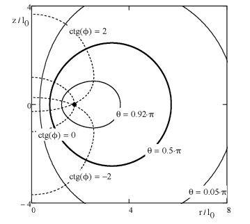
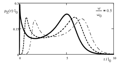
Figure 2: Contours of the angles parameterizing the unit vector ${\bf n^{*}}$ for $H=3$ and $\omega/\omega_{0}=0.5$. The solid and dashed curves correspond to $\theta=const$ and $ctg(\phi)=const$, respectively.

Figure 3: Distance dependence of the normalized energy density for solitons with the same precession frequency for various $H$ values. The solid, dashed, and dash dotted curves correspond to $H=2$, $3$, and $4$, respectively.

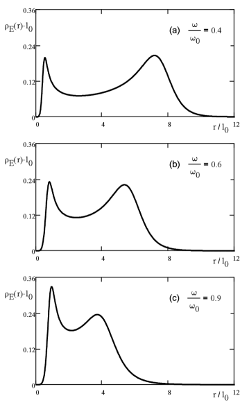
Figure 4: Distance dependence of the normalized energy density of a soliton for several values of the precession frequency and $H=3$.

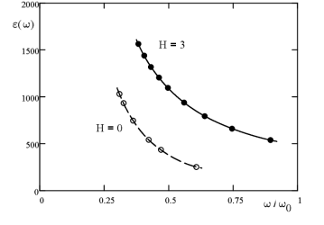
Figure 5: Energy versus the precession frequency for nontopological ($H=0$) and topological ($H=3$) solitons. The points show the numerical results.

The formula describing the Hopf index simplifies drastically for fields specified by Eqs. (6) bib:KUR ; bib:Glad

$$H=QT,$$ (13)

where the integer $T$ is given by

$$T=\frac{1}{4\pi}\int_{-\infty}^{\infty}{\int_{0}^{\infty}{{\bf n^{*}}\cdot\left[\frac{\partial{\bf n^{*}}}{\partial r}\times\frac{\partial{\bf n^{*}}}{\partial z}\right]}d{r}}d{z}.$$ (14)

To solve the variational problem numerically by the finite difference method, the energy functional was replaced by a function of the projections of the vector ${\bf n^{*}}$ at the numerical-grid nodes. Since the field configuration for negative $z$ values is determined by the symmetry of the problem, the discretization domain was the unit square $0\leq r\leq 1,0\leq z\leq 1$.

The expected domain of soliton localization should be about the typical scale

$$l_{0}=\sqrt{\frac{\alpha}{\beta}}.$$ (15)

The parameters $\alpha$ and $\beta$ were chosen to ensure that $1/l_{0}\sim\sqrt{D}$, where $D$ is the number of grid nodes in one direction. The key point of this method is to ensure that the soliton is entirely contained in the simulation domain, but is sufficiently large to be adequately described by the discrete grid. In addition, to improve the performance, the numerical grid was nonuniform with the density of nodes increasing toward the coordinate origin. This means that the inhomogeneity was assumed to be localized near the center, while the field quickly reaches the asymptotic uniform state at infinity. The vector ${\bf n_{0}}=(0,0,1)$ at the boundaries $z=1$ or $r=1$ of the domain corresponds to the ground state.

The energy with an additive penalty function was minimized by the conjugate gradient method. A quadratic penalty function imposes a constraint on the norm of the vector ${\bf n^{*}}$ which is unity at any point. Integral (7) is discretized to a linear form, and the imposed constraint is taken into account by applying a linear operator bib:PD in the calculation of the direction toward the minimal objective function for each iteration.

A feature of our numerical analysis was the choice of the initial state, i.e., the trial field configuration from which the minimization begins. The vector corresponded to the ground state in the entire domain of simulation excluding a small quadrant near the coordinate origin. The vectors inside the quadrant lied in the orthogonal plane, and their directions varied randomly from point to point. Thus, the initial configuration is to a certain extent chaotic and does not even obey the criteria for the discretization of any smooth function.

The result was directly tested in addition to the observed approach of the energy to its asymptotic value after many iterations. The frequency $\omega$ was calculated using Eq. (9). The second derivatives and the discrepancy of Landau-Lifshitz equation (2) were numerically evaluated at each internal point of the simulation domain.

For the solitons presented below, the numerical calculations based on Eq. (14) yielded $T=1$. In this case, according to Eq. (13), the Hopf index $H=Q$. Topological solitons of other types will be described elsewhere. The results of our present study are discussed below.

Figure 1 shows a typical configuration of the field $\bf{n}$ for $H=3$. Here, the coordinate axes are shifted for clarity and illustrate only the spatial orientation of the soliton. It is seen that the linking number of the preimages of two points of the $S^{2}$ sphere is equal to three. The toroidal surface corresponds to $\theta=\pi/2$. Note that ${\bf n}={\bf n}_{0}$ on the symmetry axis $r=0$ and ${\bf n}\rightarrow{\bf n}_{0}$ for $r^{2}+z^{2}\rightarrow\infty$.

The contours of the angles parameterizing the vector ${\bf n^{*}}$ are plotted in Fig. 3. The curve $\theta=\pi/2$ is a section of an axisymmetric surface of kind 1 (toroidal surface) in which a large fraction of the soliton energy is contained. The common point of the lines $\phi=const$ is the south pole of the sphere $S^{2}$, at which $\theta=\pi$.

Analysis showed that it is most difficult to simulate solitons with small H values. A series of efficacious numerical results were obtained for $H=3$ and $4$ using a 600x400 grid. However, in the case where $H=2$, a plausible result was obtained only for a 1600x800 grid. The cause is an interesting feature of the structure of the studied class of objects. This feature becomes apparent in numerical calculations of the normalized energy density

$$\rho_{E}=\frac{1}{E}\int_{-\infty}^{\infty}w_{E}d{z}.$$ (16)

The dependences of $\rho_{E}$ on $r$ for various values of $H$ are plotted in Fig. 3. The maximum $\rho_{E}$ values are reached in the vicinity of $\theta=\pi/2$. With a decrease in $H$, the localization domain corresponding to the first maximum of $\rho_{E}(r)$ becomes narrower and the maximum becomes steeper. The soliton structure becomes narrower, so that a finer grid with more nodes should be used.

Three-dimensional solitons with $H=0$ exist for $\omega\leq 0.915\omega_{0}$  bib:IvKos1 , where $\omega_{0}$ is the ferromagnetic-resonance frequency:

$$\omega_{0}=\frac{2\mu_{0}M_{0}\beta}{\hbar}$$ (17)

An increase in the precession frequency results in the compression of the soliton (Fig.4) implying the possible existence of certain threshold ratio $\omega/\omega_{0}$ similar to the nontopological soliton bib:IvKos1 .

Figure 5 shows the dimensionless energy $\varepsilon={E}/(\alpha l_{0})$ as a function of $\omega/\omega_{0}$. It is seen that the soliton energy decreases with an increase in the precession frequency. A similar dependence for a magnon drop, calculated by the aforementioned procedure, is shown in this figure for a comparison.

The discovered solitary structures with typical sizes of a few to a few tens of $l_{0}$ are much smaller than cylindrical magnetic domains and, therefore, can potentially be used for information recording and storage if mechanisms for their generation and control will be developed in the same way as it is done now for magnetic vortices bib:OBS . This would provide the possibility of recording information in three-dimensional samples.

References

-
(1)
R. Bott and L. W. Too, Differential Forms in Algebraic Topology, 1982, New York.
-
(2)
L. D. Faddeev, IAS Princeton, IAS-Report No.75-QS70, (1975).
-
(3)
L. D. Faddeev,
A. J. Niemi,
Nature 387,
58 (1997).
http://arxiv.org/abs/hep-th/9610193.
-
(4)
L. D. Faddeev,
A. J. Niemi,
hep-th/9705176,
(1997).
http://arxiv.org/abs/hep-th/9705176.
-
(5)
R. A. Battye,
P. M. Sutcliffe,
Phys. Rev. Lett. 81,
4798 (1998).
http://prola.aps.org/abstract/PRL/v81/i22/p4798_1,
http://arxiv.org/abs/hep-th/9808129.
-
(6)
J. Gladikowski,
M. Hellmund,
Phys. Rev. D 56,
5194 (1997).
http://prola.aps.org/abstract/PRD/v56/i8/p5194_1,
http://arxiv.org/abs/hep-th/9609035.
-
(7)
G. E. Volovik,
V. P. Mineev,
Sov. Phys. JETP 46,
401 (1977).
-
(8)
I. E. Dzyloshinskii,
B. A. Ivanov,
JETP Lett. 29,
540 (1979).
http://jetpletters.ac.ru/ps/1455/article_22156.shtml
-
(9)
G. M. Derrick,
J. Math. Phys 5,
1252 (1964).
http://link.aip.org/link/?JMAPAQ/5/1252/1.
-
(10)
A. M. Kosevich,
B. A. Ivanov,
A. S. Kovalev,
Phys. Rep. 194,
117 (1990).
http://dx.doi.org/10.1016/0370-1573(90)90130-T.
-
(11)
N. Papanicolaou,
T. N. Tomaras,
Nucl. Phys. B 360,
425 (1991).
http://dx.doi.org/10.1016/0550-3213(91)90410-Y.
-
(12)
T. Okuno,
K. Mibu,
T. Shinjo,
J. Appl. Phys 95,
3612 (2004).
http://link.aip.org/link/?JAPIAU/95/3612/1.
-
(13)
G. E. Volovik,
cond-mat/0701180,
(2007).
http://arxiv.org/abs/cond-mat/0701180.
-
(14)
Yu. M. Bunkov,
G. E. Volovik,
Phys. Rev. Lett. 98,
265302 (2007).
http://link.aps.org/abstract/PRL/v98/e265302,
http://arxiv.org/abs/cond-mat/0703183.
-
(15)
Yu. M. Bunkov,
G. E. Volovik,
J. Low Temp. Phys 150,
135 (2008).
http://www.springerlink.com/content/a55n5722617l68k8,
http://arxiv.org/abs/0708.0663.
-
(16)
Yu. M. Bunkov,
G. E. Volovik,
Physica C 468,
609 (2008).
http://dx.doi.org/10.1016/j.physc.2007.11.026,
http://arxiv.org/abs/0710.3448.
-
(17)
A. B. Borisov,
JETP Lett. 76,
84 (2002),
http://www.springerlink.com/content/g48t670u4906110h.
-
(18)
N. R. Cooper,
Phys. Rev. Lett. 82,
1554 (1999),
http://link.aps.org/abstract/PRL/v82/p1554,
http://arxiv.org/abs/cond-mat/9901037.
-
(19)
B. A. Ivanov,
A. M. Kosevich,
JETP Lett. 24,
495 (1976).
http://jetpletters.ac.ru/ps/1816/article_27757.shtml.
-
(20)
T. Ioannidou,
P. M. Sutcliffe,
Physica D 150,
118 (2001).
http://dx.doi.org/10.1016/S0167-2789(00)00221-9,
http://arxiv.org/abs/cond-mat/0101129.
-
(21)
P. M. Sutcliffe,
Phys. Rev. B 76,
184439 (2007).
http://link.aps.org/abstract/PRB/v76/e184439,
http://arxiv.org/abs/0707.1383.
-
(22)
A. Kundu,
Y. P. Rybakov,
J. Phys. A 15,
269 (1982).
http://www.iop.org/EJ/abstract/0305-4470/15/1/035.
-
(23)
J. Tjon,
J. Wright,
Phys. Rev. B 15,
3470 (1977).
http://link.aps.org/abstract/PRB/v15/p3470.
- (24) B. N. Pshenichnyi and Yu. M. Danilin, Numerical Methods in Extremal Problems (Nauka, Moscow, 1975) [in Russian].