Injected Power Fluctuations in 1D dissipative systems : role of ballistic transport

Abstract

This paper is a generalization of the models considered in [J. Stat. Phys. 128,1365 (2007)]. Using an analogy with free fermions, we compute exactly the large deviation function (ldf) of the energy injected up to time $t$ in a one-dimensional dissipative system of classical spins, where a drift is allowed. The dynamics are $T=0$ asymmetric Glauber dynamics driven out of rest by an injection mechanism, namely a Poissonian flipping of one spin. The drift induces anisotropy in the system, making the model more comparable to experimental systems with dissipative structures. We discuss the physical content of the results, specifically the influence of the rate of the Poisson injection process and the magnitude of the drift on the properties of the ldf. We also compare the results of this spin model to simple phenomenological models of energy injection (Poisson or Bernoulli processes of domain wall injection). We show that many qualitative results of the spin model can be understood within this simplified framework.

I Introduction

Dissipative systems are generically systems for which a few relevant degrees of freedom can be singled out and obey closed dynamical equations: typically a fluid, where the velocity field obeys the Navier-Stokes equation, belongs to this category. Another well-known example is given by granular materials, where the identification of relevant variables (collisions) is even more evident. The lack of completeness, caused by the selection of some degrees of freedom, gives however these systems a nonconservative character, as energy flows continuously from relevant degrees of freedom (kinetic energy) to irrelevant ones (thermal agitation). As a result, the dissipative systems are by nature very different from the systems usually suitable for the use of classical statistical physics, where the conservation of energy is an unavoidable assumption. In particular, the whole set of tools devised by statistical physics can be of questionable use, even in situations where a statistical approach seems natural: it is very tempting to interpret turbulent systems, or a vibrated granular matter, in terms of effective temperature, correlations, Boltzmann factor, etc…but the soundness of such an approach is often questionable.

Quite recently, the interest of physicists has been drawn to the injection properties of dissipative systems for several reasons. First, it was easily measurable experimentally, and the measurements showed that, contrarily to what was usually expected, the injected power fluctuates a lot, is not Gaussian, and does not obey the usual simple scaling arguments fauveexp1 ; fauveexp2 . Moreover, the injection is by nature very important in dissipative systems, since it is required to draw the system out of rest; thus, it is natural to study specifically this observable, which is at the same time responsible for the existence of the stationary state, and is strongly affected by it aumaitrefauvemcnamarapoggi . Finally, some theoretical works on the so-called “Fluctuations Theorems” had suggested a possible symmetry relation in the distribution of the fluctuations of the injected power, a suggestion vigourously debated since the works of aumaitrefauvemcnamarapoggi ; evanscohenmorris ; gallavotticohen ; kurchan ; kurchanrevue ; cilibertolaroche .

In studying the fluctuations of global (macroscopic) variables of a disordered (turbulent) dissipative system, one faces soon a crucial problem: contrary to the statistical physics of conservative systems, no global theory is at hand here to predict the level of fluctuations, the physical meaning of their magnitude, the skewness of the distributions, etc…All these features are intimately connected to the statistical stationary turbulent state, but in a way nowadays beyond our knowledge. A way to make progress towards a better understanding of these issues is to consider toy-models of dissipative systems where some features of real systems are reproduced, and analyze the structuration of the stationary states. If one can find for these systems an intimate connection between their injection properties and their dynamical features, such rationale could perhaps be adapted to more realistic systems. Such a procedure has been successfully applied in the study of fluctuations of current for conservative systems bodineauderrida .

In this paper, which follows a former one faragopitard , we study a one-dimensional model of dissipative system, which has the advantage to allow for an exact description. This model consists of a chain of spins subject to an asymmetric $T=0$ Glauber dynamics, and is driven out of rest by a Poissonian flip of one spin (see next section for details): this is one of the rare examples where a nontrivial stationary dissipative state can be entirely described. In fact, we generalized the symmetric model studied in faragopitard by allowing for an asymmetry in the diffusion dynamics. This system is, in comparison with real dissipative systems, ridiculously simple, but one can hope that such examples would give ideas to interpret real experiments or to explain measurements on other variables, correlations, etc…For that purpose, this paper focuses much more on the physical content of the results than on the computational details, that are postponed in the appendix. More precisely, the observable we look at is the energy $\Pi$ provided to the system by the injection mechanism between $t$ and $t+\tau$ in the permanent regime. For large $\tau$, the probability distribution function (pdf) of $\Pi$ obeys the large deviation theorem and the probability distribution function is entirely governed by the large deviation function $f$ (introduced below). The procedure of integrating the observable of interest over time has at least two advantages. First, one can hope that this effective low-frequency filter fades away “irrelevant” details of the dynamics and provides information on large-scale, hopefully more universal phenomena at work; this statement has been proved correct in some cases farago1 ; bodineauderrida . Secondly, the experiments are always constrained by a finite maximal frequency for the sampling of the time series: in practice the typical sampling time is much larger than the fastest relaxation times of the system under consideration. As a result, the pdfs experimentally measured are necessarily related to time integrated variables. The large deviation function is a good representation of these pdfs in the case where the sampling frequency is small with respect to the dynamics of the bulk.

The paper is organized as follows: in the next section we define precisely the model; sections III and IV are devoted to the physical results given by our computations. In section V, we show that the main characteristics of the large deviation function of the injected power are explained quite well using a simple phenomenological model, which treats the correlations between the boundary and the bulk in an effective way. The appendix (section VII) gives in detail all the steps of the computation, based on a free-fermion approach of the intermediate structure factor.

II The model

We consider a 1D system of $N+3$ ($N\rightarrow\infty$) classical spins on a line, labelled from $-1$ to $N+1$. The values of the extremal spins $s_{-1}$ and $s_{N+1}$ are fixed (this choice makes the description in terms of domain walls easier, as explained in the appendix). The zeroth spin $s_{0}$ is the locus where energy is injected into the system: the flipping of $s_{0}$ is just a Poisson process with rate $\lambda$, independent of the state of the other spins. The spins of the “bulk”, from $s_{1}$ to $s_{N-1}$ are updated according to an asymmetric $T=0$ Glauber dynamics.

The asymmetric $T=0$ Glauber dynamics is defined as follows : given $0<p<1$, the probability for a spin $s_{j}$ to flip between $t$ and $t+dt$ is

$$dt[1-s_{j}([1-p]s_{j-1}+ps_{j+1})],$$ (1)

which is illustrated in figure 1.

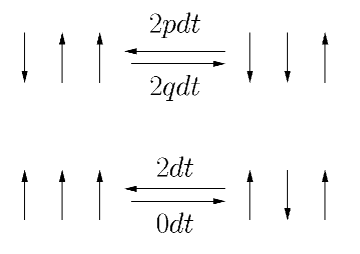
Figure 1: The rates of the asymmetric Glauber dynamics

Note that if $p>q$ (resp. $<$), the domain walls are locally drifted to the left (resp. right); for $p=q=1/2$ we recover the system studied in faragopitard (with the difference, that contrarily to faragopitard the system is not duplicated on each side of $s_{0}$; this simplification yields simpler calculations and a physics a bit easier to analyze). Note that the case $p<1/2$, where the domain walls easily invade the system, is probably the most relevant one for a comparison with experimental devices of turbulent convection.

These dynamics are dissipative but a non trivial stationary state is nervertheless reached thanks to the Poisson process on $s_{0}$ which injects continuously energy into the system (the injected energy is positive on average; however, negative energy injections are also possible fluctuations due to the bulk dynamics).

III The mean injected power

The mean value of the injected power $\langle\varepsilon\rangle$ can easily be calculated. It is given by $\langle\varepsilon\rangle=\lambda[\text{Prob}(s_{0}=s_{1})-\text{Prob}(s_{0}=-s_{1})]=\lambda\langle s_{0}s_{1}\rangle$. To compute $U_{j}=\langle s_{0}s_{j}\rangle$ (we are interested here in the special case $j=1$), we notice that the quantity $U_{j}$ obeys a closed equation in the permanent regime (see farago1 for details):

$$-(\lambda+1)U_{j}+pU_{j+1}+qU_{j-1} =0$$ (2)

(let us recall that $q=1-p$) with the boundary conditions $U_{0}=1$ and $U_{\infty}=0$. The determination of $U_{j}$ is simple : the polynomial $pX^{2}-X(\lambda+1)+q$ has a unique root $r$ less than one, and therefore $U_{j}=r^{j}$. The mean injected power

$$\langle\varepsilon\rangle =\lambda\frac{\lambda+1-\sqrt{(\lambda+1)^{2}-4pq}}{2p}$$ (3)

is plotted in figure 2. One can see that it is an increasing function of $\lambda$ and a decreasing function of $p$. This last point can be easily understood, as for higher $p$ the domain walls are more and more confined near the boundary, enhancing the probability of negative energy injection. On the contrary, for low values of $p$, the domain walls invade the system rather easily: for $p<1/2$, they are drifted away from the site of injection. This is at the origin of a large positive value for the average injection energy.

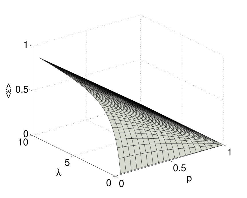
Figure 2: Mean injected power as a function of $\lambda$ and $p$.

IV The large deviations of the injected power

The main result of our paper is the computation of $f(\varepsilon)$, the large deviation function of the injected energy. This is a central observable associated with the long time (or low frequency) properties of the fluctuations of the energy flux in stationary systems. Let us call $\Pi$ the energy injected into the system between $t=0$ and $t=\tau$; typically $\Pi$ scales like $\tau$ for large $\tau$. The ldf $f(\tau)$ is defined as

$$f(\varepsilon)=\lim_{\tau\rightarrow\infty}\tau^{-1}{\ln[\text{Prob}(\Pi/\tau=\varepsilon)]}$$ (4)

However it is simply defined, this quantity is difficult to compute or analyze theoretically, as it involves the knowledge of the complete dynamics of the system, and measures the temporal correlations which develop in a nontrivial way in the nonequilibrium stationary state.

Usually, one computes first the ldf $g(\alpha)$ associated with the generating function of $\Pi$:

$$\langle e^{\alpha\Pi}\rangle{\displaystyle\mathop{\simeq}_{\tau\rightarrow\infty}}e^{\tau g(\alpha)}$$ (5)

More precisely $g(\alpha)=\lim_{\tau\rightarrow\infty}\tau^{-1}\log\langle e^{\alpha\Pi}\rangle$. Then, $f(\varepsilon)$ can be obtained numerically solving the inverse Legendre transform

$$f(\varepsilon) =\min_{\alpha}\left(g(\alpha)-\alpha\varepsilon\right)$$ (6)

The details of the computation of $g(\alpha)$ are postponed in the Appendix. The formula for $g(\alpha)$ (equation (85)) is not easy to interpret physically. We are thus in a situation where the exact result does not really highlight the underlying physics, and in particular does not make the long-time properties of the injection process particularly transparent. In order to clarify this, we will follow a very pragmatic way: first we will sketch the different ldfs corresponding to different values of the relevant parameters $(\lambda,p)$ and raise some questions associated to them. In the next section, we will see that some simple phenomenological models account very well for the observed behaviours (these models were neither discussed nor even evoked in faragopitard ).

In figure 3 (a), we show various functions $f(\varepsilon)$ for different values of the parameters $\lambda$ and $p$, as a function of $\varepsilon/\langle\varepsilon\rangle$. $f(\varepsilon)$ is maximum for $\varepsilon=\langle\varepsilon\rangle$, which is a generic property of ldfs.

Figure 3: (Color online) Large deviations functions $f(\varepsilon)$ as a function of $\varepsilon/\langle\varepsilon\rangle$ for various values of the parameters $p$ and $\lambda$. (a) curvature not rescaled, (b) curvature normalized

Clearly, the curvature at the maximum is a major feature of these curves, and is strongly dependent on the parameters $(\lambda,p)$. Writing $f(\varepsilon)=-\frac{1}{2}[-f^{\prime\prime}(\langle\varepsilon\rangle)\langle\varepsilon\rangle^{2}](\varepsilon/\langle\varepsilon\rangle-1)^{2}+o(\varepsilon/\langle\varepsilon\rangle-1)^{2}$, we see that the relevant quantity associated to the curvature, once $\varepsilon$ has been rescaled by $\langle\varepsilon\rangle$, is $\sigma=-f^{\prime\prime}(\langle\varepsilon\rangle)\langle\varepsilon\rangle^{2}=g^{\prime}(0)^{2}/g^{\prime\prime}(0)$. The curves rescaled by the curvature $\sigma$ are plotted in figure 3 (b), where it is seen that the curvature and the mean energy, though of primordial importance, are however not sufficient to characterize fully the ldf: there is no clear collapse of the curves. The dependence of $\sigma$ with respect to $p$ and $\lambda$ is plotted in figure 4 (a).

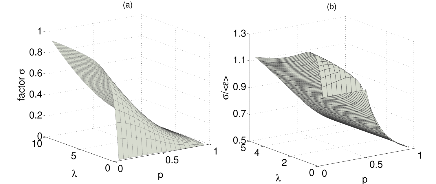
Figure 4: (a) Factor $\sigma=-f^{\prime\prime}(\langle\varepsilon\rangle)\langle\varepsilon\rangle^{2}$ and (b) Fano factor $\sigma/\langle\varepsilon\rangle$, as a function of $\lambda$ and $p$.

Its behaviour is remarkably similar to that of $\langle\varepsilon\rangle$ itself. Before explaining this point (see next section), we note that the mean value of the energy injected up to time $\tau$ is $\langle\Pi\rangle=\tau\langle\varepsilon\rangle$; besides, the (squared) relative fluctuations of this quantity is given for large $\tau$ by $[\langle\Pi^{2}\rangle-\langle\Pi\rangle^{2}]/\langle\Pi\rangle^{2}=1/(\tau\sigma)$. The ratio of these two quantities $[\langle\Pi^{2}\rangle-\langle\Pi\rangle^{2}]/\langle\Pi\rangle=\sigma/\langle\varepsilon\rangle$, called the Fano factor, is plotted in figure 4 (b): it is comprised between 0.5 and 1.3 for all values of the parameters $(\lambda,p)$, which shows that the correlation between $\sigma$ and $\langle\varepsilon\rangle$, though clearly demonstrated, is a bit loose. Thus, a sound question is to ask why $\sigma$ and $\langle\varepsilon\rangle$ are correlated, and what are the factors which limit or modulate this correlation. These issues will be discussed in the next section.

Let us go back to the rescaled ldf in figure 3 (b). One can notice that all curves display a noticeable counterclockwise tilt with respect to the parabola. As for the Fano factor, this tilt seems to be constant, with some minor relative differences. To quantify this tilt, one writes the Taylor expansion of $f(\varepsilon)/\sigma$ up to the third order like:

$$f(\varepsilon)/\sigma=-\frac{1}{2}(\varepsilon/\langle\varepsilon\rangle-1)^{2}+\frac{\chi}{6}(\varepsilon/\langle\varepsilon\rangle-1)^{3}+o(\varepsilon/\langle\varepsilon\rangle-1)^{3}$$ (7)

A simple calculation gives $\chi=g^{\prime\prime\prime}(0)g^{\prime}(0)/g^{\prime\prime}(0)^{2}$. This parameter quantifies the tilt and can be a priori positive or negative. The variation of $\chi$ with $(p,\lambda)$, plotted in figure 5,

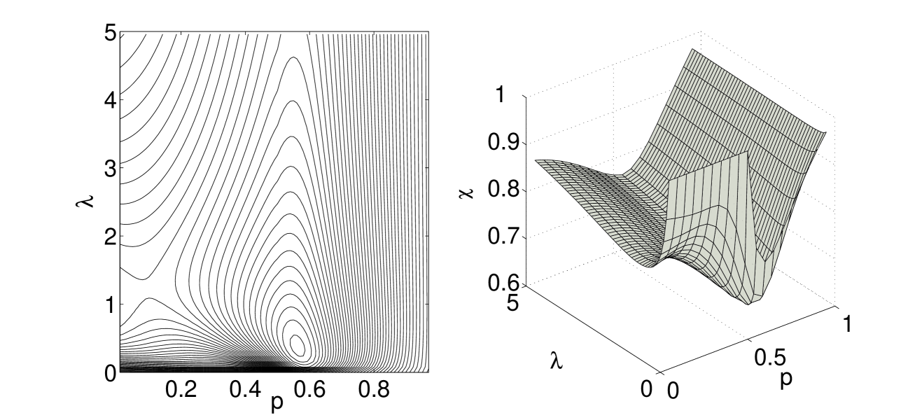
Figure 5: Parameter $\chi$ as a function of $p$ and $\lambda$. The left graph is a contour plot of the surface.

shows a rather complicated dependence of $\chi$ with respect to the parameters (in particular an absolute minimum for $p\sim 0.6$ and $\lambda\gtrsim 0.5$), but with always $\chi\in[0.6,1]$. Both the global trend and the finer details raise natural questions: why is the tilt is always positive ? What does it mean concerning the physics of the system ? Why is the dependence on $p$ and $\lambda$ so complicated ? The next section provides a phenomenological model which give satisfactory answers to these issues .

V Discussion and comparison with a simplified model

In this section we compare the results obtained above to a very simple model, in order to see which global mechanisms are at work.

We consider an oversimplified version of our system, called in the following “pure Poissonian model” or PPM. In this model, the injection is a Poissonian emission (with rate $\rho$) of domain walls (d.w.) into the system and the energy is incremented by one each time a d.w. is emitted. In this case, on has $\langle\Pi\rangle=\tau\rho$ and $[\langle\Pi^{2}\rangle-\langle\Pi\rangle^{2}]/\langle\Pi\rangle^{2}=1/(\tau\rho)$, that is $\langle\varepsilon\rangle$ and $\sigma$ are both equal to $\rho$. Thus, in our system, the global similarity between the two quantities, i.e. $\sigma/\langle\varepsilon\rangle\sim 1$ is not fortuitous, it is in fact a signature of the approximate Poissonian structure of the injection.

Conversely, the violation of the relation $\sigma/\langle\varepsilon\rangle=1$, plotted in figure 4 (b), is interesting, as it accounts directly for the coupling of the Poissonian injection and the structuration of the system near the boundary. In order to clarify this coupling, we can extend slightly the PPM to account for the variability of the Fano factor, by considering that in an “effective” energy injection, not only one domain wall is concerned, but in fact an average number of domain walls $n_{\text{dw}}$. For instance, for $p\simeq 1$, where the domain walls are confined at the boundary, the only way for the system to absorb energy is the following rare event: a domain wall is created between $s_{0}$ and $s_{1}$, it translates to the right (limiting factor), and then comes back to annihilate with another entering domain wall. This “injection event” is so rare, that two such events are necessarily far apart from each other, and the statistics of these events is actually Poissonian. In fact, one can see that the effective number of domain walls associated to one event is two instead of one. Indeed, if one generalizes the PPM to emit $n_{\text{dw}}$ domain walls per event, one gets $\sigma/\langle\varepsilon\rangle=1/n_{\text{dw}}$: figure 4 (b) gives $n_{\text{dw}}\simeq 2$ in the $p\simeq 1$ region as expected.

Another region is simple to analyze: for $\lambda\simeq 0,p<0.5$ (the domain walls invade the bulk), the inner dynamics is so slow that the effective emission of domain walls invading the bulk is Poissonian; virtually no domain wall is reabsorbed by the boundary. One understands that this scenario breaks down rather abruptly when the drift is directed towards $s_{0}$, which explains the singular behaviour of the Fano factor at $(\lambda,p)=(0,0.5)$. To summarize, the fact that $\sigma/\langle\varepsilon\rangle<1$ for the most part of the parameter range illustrates the cooperative character of the energy injection.

However, in the special case of large $\lambda$, small $p$, one also expects a Poissonian behaviour, determined in this case by the natural time of the bulk dynamics: for very quick flipping of the spin $s_{0}$, and $p\gtrsim 0$, the emission of a domain wall into the system is only limited by the move of the first domain wall to the right.

The PPM, even modified by the parameter $n_{\text{dw}}$ is unable to account for the region where the Fano factor is larger than one (namely this regime of large $\lambda$, small $p$): it is difficult to imagine an effective Poissonian emission of an average number of domain walls less than one. Moreover, if one also considers also the tilt parameter $\chi$, the disagreements are stronger, for it can be easily shown that the PPM (with $n_{\text{dw}}$ allowed) yields $\chi=1$, irrespective of the value of $n_{\text{dw}}$. We conclude that if the global trend of a positive tilt is again a signature of the approximate Poissonian nature of the domain wall injection, the model is a bit too rough to account for the observed subtleties (except for regions where $\chi\simeq 1$, which correspond to the cases commented above).

In order to get a finer description of the phenomenology, we can add a new parameter in the PPM model. Instead of assuming a Poisson process for the emission of domain walls, we assume a Bernoulli process bernoulli : the time span $[0,t]$ is divided into $t/\Delta t$ intervals of length $\Delta t$, during which $n_{\text{dw}}$ domain walls can be emitted with a probability $\rho\Delta t$. One thus takes into account a possible waiting time after an emission event during which no other event is on average allowed. For this model, one easily shows that

$$\langle\varepsilon\rangle =\rho n_{\text{dw}}$$ (8)

$$\sigma/\langle\varepsilon\rangle =\frac{1}{n_{\text{dw}}(1-\rho\Delta t)}$$ (9)

$$\chi =\frac{1-2\rho\Delta t}{1-\rho\Delta t}$$ (10)

We remark that now the Fano factor can reach values less than one. This is the case for small values of $\lambda$ and $p<1/2$, where $n_{\text{dw}}$ is certainly one: here the Poissonian character of the process is imposed by $\lambda$, but there can be a waiting period after a flipping of $\lambda$, due to the finite time required for the bulk dynamics to remove the domain wall from its first position.

We remark also that the $\chi$ factor of the Bernoulli model is always less than one, exactly like in the real system. It confirms also our previous interpretation for the case $\lambda\simeq 0$ and $p<1/2$: a deep decrease of $\chi$ is observed for increasing values of $\lambda$, which is associated in the Bernoulli model with an increase of $\Delta t$. By the way, we can extract from the preceding equations the effective parameters $n_{\text{dw}}$, $\Delta t$ and $\rho$, knowing $\langle\varepsilon\rangle$, $\sigma$ and $\chi$ from our numerical computation:

$$\Delta t =\frac{1-\chi}{\sigma}$$ (11)

$$n_{\text{dw}} =(\sigma/\langle\varepsilon\rangle)^{-1}(2-\chi)$$ (12)

$$\rho =\frac{\sigma}{2-\chi}$$ (13)

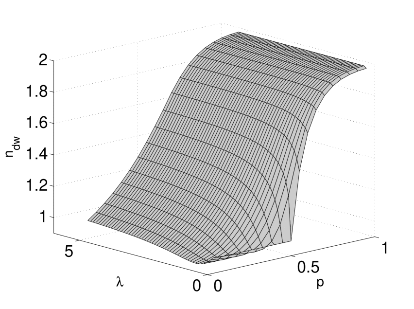
Figure 6: Effective parameter $n_{\text{dw}}$ as a function of $p$ and $\lambda$.

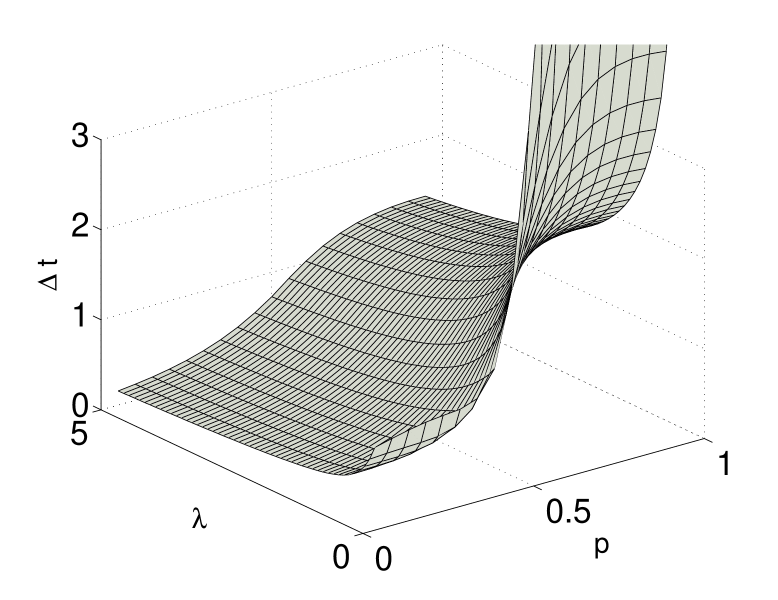
Figure 7: Effective parameter $\Delta t$ as a function of $p$ and $\lambda$.

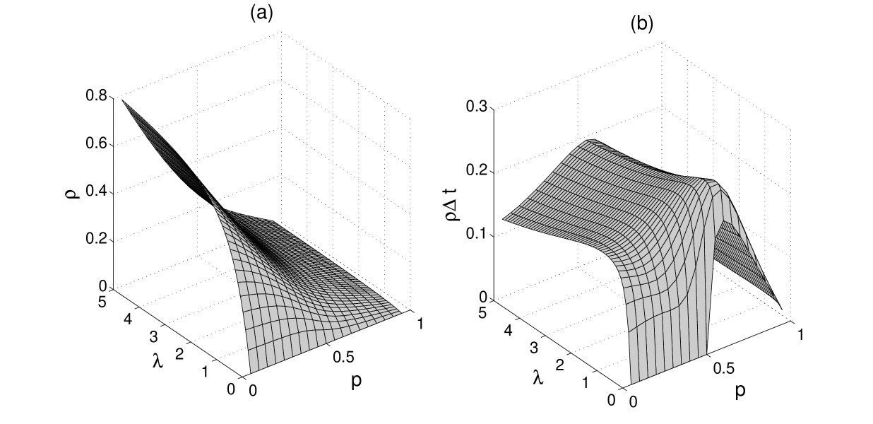
Figure 8: Effective parameters (a) $\rho$ and (b) $\rho\Delta t$ as a function of $p$ and $\lambda$.

In figure 6, 7, 8 (a) and 8 (b), we see the values of $n_{\text{dw}}$, $\Delta t$, $\rho$ and $\rho\Delta t$ respectively, extracted from the results for the spin model. The interpretation of figure 6 is obvious: as expected, the average number of domain walls $n_{\text{dw}}$ stays close to one for $p\gtrsim 0$ and all values of $\lambda$, and reaches 2 for $p\simeq 1$, the intermediate $p$ values corresponding to a crossover region.

The quantities $\rho^{-1}$ and $\Delta t$ are both related to the natural timescale of the effective injection process. The main difference between them is that $\rho^{-1}$ is effectively the rate of the equivalent process, whereas $\Delta t$ is somehow a “waiting time” during which two injection events have little chance to occur consecutively. $\Delta t$ is plotted in figure 7.

Figure 8 (a) shows as expected that the injection process is very inefficient for $\lambda\simeq 0$ and also for $p\simeq 1$; obviously, this curve is qualitatively related to $\langle\varepsilon\rangle$, since the efficiency of the injection has immediate consequences on the mean injected power, but it is interesting to note that $\rho$ is by no means constructed from $\langle\varepsilon\rangle$, but from cumulants of higher order.

Figure 8 (b) shows that the system is really Poissonian in the regions $(\lambda\gtrsim 0,p<1/2)$ and $p\lesssim 1$, despite the fact that $\Delta t$ can be large (fig. 7). Note also the vicinity of $\lambda=0$ and $p>1/2$, where something interesting happens: two factors that elsewhere favours the Poisson character of the process, namely $\lambda$ small and $p>1/2$, are simultaneously at work here and act again each other. The results of this “collision” is that the process is clearly not Poisson for $p$ around $0.8$, due to huge values of $\Delta t$ (see fig. 7); this is also a transitional region from a Poisson process with one domain wall to a Poisson process with two domain walls.

Finally, when $p<1/2$ and $\lambda$ is away from zero (this is the region where the Fano fctor is larger than $1$), we find a non Poissonian process with $\Delta t$ of the order of $10\%$ to $15\%$ of $\rho^{-1}$. For instance, when $p=0$, $\rho$ increases as $\lambda$ increases: there is a crossover from a $\lambda$-limited regime to a bulk-limited regime for which a waiting time is observed. In this case, the probability of two close injection events is weakened because an injection event uses two spin flips: one flips of $s_{0}$ and then a flip of $s_{1}$ (for $p=0$, $s_{1}$ can flip only if $s_{1}=-s_{0}$); thus the probability of two events within $\delta t$ goes like $\lambda^{2}(\delta t)^{4}$ instead of $(\rho\delta t)^{2}$ for a pure Poisson process (PPM). This explains the emergence of the waiting time.

VI Conclusion

In this paper, we have presented a one-dimensional model of a dissipative system, a half infinite chain of spins at $T=0$ in a Glauber dynamics with a drift toward or away the boundary, sustained in a nontrivial stationary state by an injection mechanism, namely the Poissonian flipping of the boundary spin. We computed exactly the large deviation function of the injected power and subsequently the first three cumulants of its probability distribution, which account for the mean value of the injected power, its fluctuations and the skewness of the fluctuations. Using a simple phenomenological model and its refined version, we have shown that it can account for the main physical characteristics of the injection process very convincingly, allowing for a relevant physical interpretation of the variations of the three cumulants with the parameters $(\lambda,p)$ (rate of $s_{0}$ flipping, magnitude of the drift), in terms of an effective rate of emission of energy “quanta”, an average number of domain walls in each quantum, and a possible waiting time after an injection event.

We can hope that this phenomenology could give an interesting scheme to interpret some experiments, where the same kind of injection mechanism is more or less reproduced. For instance, in a turbulent experiment, unpinning of vortices created near a moving boundary could be a process of energy injection suitable for the description framework that we propose here. We can also think of the bubble regime in the ebullition process, where the main part of the energy transfer occurs via unpinning of vapour bubbles. We hope that some experimental results aumaitrefauve could find a simple interpretation in the kinetic description that we give here.

Finally our mathematical calculations show that such simple out-of-equilibrium models are integrable: this opens the way to more generalizations.

VII Appendix: Fermionic approach to the time-integrated injected power

It is useful to describe spin systems in the dual representation of domain walls : between the site $j$ and $j+1$ is located the possible domain wall labelled $j$ for $j=-1,\ldots N$. The state of the system is thus characterized by $\mathcal{C}=(n_{-1},\ldots,n_{N})$, where the $n_{i}$ are either 0 (no domain wall) or 1. There are $2^{N+2}$ possible states in this representation; note that the domain wall $n_{-1}$ does not play any role, but is required to make the fermionic description tractable. The dynamical equation for the probability is given by

$$\partial_{t}P(\mathcal{C})=\lambda[P(\mathcal{C}_{0})-P(\mathcal{C})]+\sum_{j=1}^{N}[P(\mathcal{C}_{j})w(\mathcal{C}_{j}\rightarrow\mathcal{C})-P(\mathcal{C})w(\mathcal{C}\rightarrow\mathcal{C}_{j})]$$ (14)

where $\mathcal{C}_{j}$ holds for the state $\mathcal{C}$ whose domain wall variables $n_{j}$ and $n_{j-1}$ have been changed (according to $n\rightarrow 1-n$). The $T=0$ asymmetric Glauber dynamics corresponds to

$$w(\mathcal{C}_{j}\rightarrow\mathcal{C}) =2[1-pn_{j}-qn_{j-1}]$$ (15)

$$w(\mathcal{C}\rightarrow\mathcal{C}_{j}) =2[pn_{j}+qn_{j-1}]$$ (16)

where $n_{j}$ and $n_{j-1}$ are the variables associated with the state $\mathcal{C}$ (we use this convention hereafter), and $q=1-p$.

We consider that each domain wall contributes as an excitation of energy $1$ to the global energy of the system. We are interested in the energy $\Pi$ injected into the system up to time $t$ by the Poissonian injection. Following derridalebowitz , the route to this time integrated observable begins with the consideration of the joint probability $P(\mathcal{C},\Pi,t)$, the probability for the system to be in the state $\mathcal{C}$ at time $t$ having received the energy $\Pi$ from the injection. The dynamical equation for this quantity is readily

$$\partial_{t}P(\mathcal{C},\Pi)=\lambda\{P(\mathcal{C}_{0},\Pi-1)n_{0}+P(\mathcal{C}_{0},\Pi+1)(1-n_{0})-P(\mathcal{C},\Pi)\}\\ +\sum_{j=1}^{N}[P(\mathcal{C}_{j},\Pi)w(\mathcal{C}_{j}\rightarrow\mathcal{C})-P(\mathcal{C},\Pi)w(\mathcal{C}\rightarrow\mathcal{C}_{j})]$$ (17)

We define next the generating function of $\Pi$ as

$$F(\mathcal{C})=\sum_{\Pi=-\infty}^{\infty}e^{\alpha\Pi}P(\mathcal{C},\Pi)$$ (18)

This quantity, summed up over the states, yields the generating function $\langle\exp(\alpha\Pi)\rangle$ from which one derives its ldf $g(\alpha)$:

$$\langle e^{\alpha\Pi}\rangle{\displaystyle\mathop{\simeq}_{t\rightarrow\infty}}e^{tg(\alpha)}$$ (19)

This ldf $g(\alpha)$ is closely related to $f(p)$, the ldf of the probability density function of $\Pi$, as they are Legendre transform of each other farago1 ; farago2 :

$$\text{Prob}(\Pi/t=p) {\displaystyle\mathop{\propto}_{t\rightarrow\infty}}\exp(tf(p))$$ (20)

$$f(p) =\min_{\alpha}\left(g(\alpha)-\alpha p\right)$$ (21)

Let us write the dynamical equation for $F$ :

$$\partial_{t}F(\mathcal{C})=\lambda\left[e^{\alpha}F(\mathcal{C}_{0})n_{0}+e^{-\alpha}F(\mathcal{C}_{0})(1-n_{0})-F(\mathcal{C})\right]\\ +2\sum_{j=1}^{N}[F(\mathcal{C}_{j})(1-pn_{j}-qn_{j-1})-F(\mathcal{C})(pn_{j}+qn_{j-1})]$$ (22)

The function $g(\alpha)$ can be expressed in terms of the linear operator acting on the “vector” $[F(\mathcal{C})]_{\mathcal{C}}$ in the r.h.s of (22) : it is in general its largest eigenvalue.

Our problem belongs to the category of the “free-fermions” problems, for which a diagonalization of the dynamics into independent “modes” can be achieved. The procedure is described in faragopitard , with references therein. In our case, the operator in the r.h.s of equation (22) can be turned into the following fermionic operator :

$$H=\lambda[e^{\alpha}c_{-1}^{\dagger}c_{0}^{\dagger}+e^{-\alpha}c_{0}c_{-1}+e^{\alpha}c_{0}^{\dagger}c_{-1}+e^{-\alpha}c_{-1}^{\dagger}c_{0}-1]\\ +2\sum_{j=1}^{N}[c_{j}c_{j-1}+qc_{j}^{\dagger}c_{j-1}+pc_{j-1}^{\dagger}c_{j}-pc_{j}^{\dagger}c_{j}-qc_{j-1}^{\dagger}c_{j-1}]$$ (23)

A symmetrisation procedure is a prerequisite to solve the problem. We define a priori the change of variables (note that the $\tilde{c}$ remain fermionic variables)

$$c_{-1}=e^{-\alpha}\tilde{c}_{-1} c^{\dagger}_{-1}=e^{\alpha}\tilde{c}^{\dagger}_{-1}$$ , (24)

$$\forall j\geqslant 1,c_{j}=u_{j}\tilde{c_{j}} c_{j}^{\dagger}=\frac{1}{u_{j}}\tilde{c}_{j}^{\dagger}$$ , (25)

where the $u_{j}$ are real quantities to be defined. The choice

$$u_{j} {\displaystyle\mathop{=}_{j\geqslant 0}}\left(\sqrt{\frac{q}{p}}\right)^{j}\equiv\nu^{j/2}$$ (26)

leads to the symmetrized expression (we omit the tildes immediately)

$$H =\lambda[e^{2\alpha}c_{-1}^{\dagger}c_{0}^{\dagger}+e^{-2\alpha}c_{0}c_{-1}+c_{0}^{\dagger}c_{-1}+c_{-1}^{\dagger}c_{0}-1]$$

$$\phantom{aaaaa}+2\sum_{j=1}^{N}[\nu^{j-1/2}c_{j}c_{j-1}+\sqrt{pq}c_{j}^{\dagger}c_{j-1}+\sqrt{pq}c_{j-1}^{\dagger}c_{j}-pc_{j}^{\dagger}c_{j}-qc_{j-1}^{\dagger}c_{j-1}]$$ (27)

$$=\sum_{n,m=-1}^{N}\left[c^{\dagger}_{n}A_{nm}c_{m}+\frac{1}{2}c_{n}^{\dagger}B_{nm}c_{m}^{\dagger}+\frac{1}{2}c_{n}D_{n,m}c_{m}\right]-\lambda$$ (28)

where $A$ is a $(N+2)\times(N+2)$ tridiagonal, real and symmetric matrix, and $B$ and $D$ $(N+2)\times(N+2)$ antisymmetric real; they are defined by

$$A =\left(\begin{array}[]{ccccccc}0&\lambda&&&&&\\ \lambda&-2q&2\sqrt{pq}&&&&\\ &2\sqrt{pq}&-2&2\sqrt{pq}&&&\\ &&2\sqrt{pq}&-2&2\sqrt{pq}&&\\ &&&\ddots&\ddots&\ddots&\\ &&&&2\sqrt{pq}&-2p\end{array}\right)$$ (35)

$$B =\left(\begin{array}[]{ccccccc}0&\lambda e^{2\alpha}&&&&&\\ -\lambda e^{2\alpha}&0&&&&&\\ &&&&&&\\ &&&\mbox{\Huge 0}&&&\\ &&&&&&\\ \end{array}\right)$$ (41)

$$D =\left(\begin{array}[]{ccccccc}0&-\lambda e^{-2\alpha}&&&&&\\ \lambda e^{-2\alpha}&0&-2\nu^{\frac{1}{2}}&&&&\\ &2\nu^{\frac{1}{2}}&0&-2\nu^{\frac{3}{2}}&&&\\ &&2\nu^{\frac{3}{2}}&0&-2\nu^{\frac{5}{2}}&&\\ &&&\ddots&\ddots&\ddots&\end{array}\right)$$ (47)

This Hamiltonian is diagonalizable, that is, it can be written

$$H =\sum_{q}\Lambda_{q}\left(\xi^{\dagger}_{q}\xi_{q}-\frac{1}{2}\right)+\underbrace{\frac{1}{2}\text{Tr}A}_{-N}-\lambda$$ (48)

where the $\xi_{q}$ are fermionic operators linearly related to the $c_{j}$ and the eigenvalues $\Lambda_{q}$ are the eigenvalues with a positive real part (we could have chosen the other half as well, see below) of the matrix

$$M_{0} =\left(\begin{array}[]{lr}A&B\\ D&-A\end{array}\right)$$ (51)

(The details of this procedure are exposed in faragopitard ; note that the lack of translational invariance prevents the use of a Fourier transformation).

The eigenvalues of $H$ are thus given by

$$\frac{1}{2}\sum_{q}\Lambda_{q}\varepsilon_{q}-N-\lambda$$ (52)

where the $\varepsilon_{q}$ are $\pm 1$. In particular, the largest eigenvalue of $H$ reads

$$g(\alpha) =\frac{1}{2}\sum_{q}\text{Re}(\Lambda_{q})-N-\lambda$$ (53)

$$=\frac{1}{4i\pi}\oint d\mu\mu\frac{\chi^{\prime}_{0}(\mu)}{\chi_{0}(\mu)}-N-\lambda$$ (54)

where $\chi_{0}$ is the characteristic polynomial of $M_{0}$ and the contour of integration is diverging half circle leant on the imaginary axis, with its curved part pointing toward the region $\text{Re}(\mu)>0$.

VII.1 The characteristic polynomial : introduction

The problem is now equivalent to finding the characteristic polynomial of $M_{0}$. We can take advantage of the emptiness of $B$. We define $E(\mu)=(A+\mu)^{-1}D(A-\mu)^{-1}$. Multiplying $\mu\text{Id}-M_{0}$ by

$$\left(\begin{array}[]{lr}(\mu-A)^{-1}&0\\ (\mu+A)^{-1}D(\mu-A)^{-1}&(\mu+A)^{-1}\end{array}\right)$$ (57)

we see that

$$\chi_{0}(\mu) =\chi_{A}(\mu)\chi_{A}(-\mu)\det(1+BE(\mu))$$ (58)

where $\chi_{A}(\mu)=\det(A-\mu)$. Besides,

$$\det(1+BE) =(1-\lambda e^{2\alpha}E_{-1,0})(1+\lambda e^{2\alpha}E_{0,-1})+\lambda^{2}e^{4\alpha}E_{0,0}E_{-1,-1}$$ (59)

$$=[1+\lambda e^{2\alpha}E_{0,-1}(-\mu)][1+\lambda e^{2\alpha}E_{0,-1}(\mu)]+\lambda^{2}e^{4\alpha}E_{0,0}(\mu)E_{-1,-1}(\mu)$$ (60)

where we exploited the fact that $E^{T}(\mu)=-E(-\mu)$. Note in passing that the symmetry of this expression with respect to $\mu\rightarrow-\mu$, is here explicit, as the $E_{jj}$ are antisymmetric functions of $\mu$.

VII.2 Some minors of $\mu\text{Id}+A$

We term $\Delta_{j}$, ($j=0,\ldots,N+1$) the determinant of the minor of $(\mu+A)$ obtained by keeping the $(N+1-j)\times(N+1-j)$ matrix located at the bottom right side of $(\mu+A)$ (one adopts the convention $\Delta_{N+1}=1$). Note that $\Delta_{N}=-2p+\mu$, $\Delta_{N-1}=(\mu-2)(\mu-2p)-4pq$, and that we have that $\det(\mu+A)=\mu\Delta_{0}-\lambda^{2}\Delta_{1}$. We have also an explicit formula, valid for $j\neq 0$:

$$\Delta_{j} =\frac{1}{1-4pqx_{+}^{2}}\left[(2qx_{+}+1)x_{+}^{j-N-1}-2qx_{+}(2px_{+}+1)(4pqx_{+})^{-j+N+1}\rule[-1.94444pt]{0.0pt}{8.88889pt}\right]$$ (61)

where $x_{+}$ is conventionally the root of the polynomial $-4pqX^{2}+(\mu-2)X-1=0$ with the largest modulus. Note that $x_{+}$ and $\Delta_{j}$ depends on $\mu$. Later on, we will denote $x_{-}=x_{+}(-\mu)$ and $\Delta_{j}^{-}=\Delta_{j}(-\mu)$; let us stress here that $x_{+}$ and $x_{-}$ are roots of different polynomials.

VII.3 The characteristic polynomial : explicit calculation

From the definition $E=(A+\mu)^{-1}D(A-\,u)^{-1}$, one gets after some computations

$$W =\frac{1}{2q}\sum_{j=1}^{N}(4q^{2})^{j}[\Delta_{j+1}\Delta_{j}^{-}-\Delta_{j+1}^{-}\Delta_{j}]$$ (62)

$$E_{0,-1} =\frac{\lambda}{\det(A+\mu)\det(A-\mu)}\left[\rule[-1.94444pt]{0.0pt}{8.88889pt}e^{-2\alpha}\Delta_{1}(\mu\Delta_{0}^{-}-\lambda^{2}\Delta_{1}^{-})+2\mu W\right]$$ (63)

$$E_{-1,-1} =\frac{-\lambda^{2}}{\det(A+\mu)\det(A-\mu)}\left[\rule[-1.94444pt]{0.0pt}{8.88889pt}(\Delta_{1}\Delta_{0}^{-}-\Delta_{1}^{-}\Delta_{0})e^{-2\alpha}+2W\right]$$ (64)

$$E_{0,0} =\frac{-\mu}{\det(A+\mu)\det(A-\mu)}\left[\rule[-1.94444pt]{0.0pt}{8.88889pt}2\lambda^{2}e^{-2\alpha}\Delta_{1}\Delta_{1}^{-}-2\mu W\right]$$ (65)

whence one deduces

$$\chi_{0}(\mu) =-\mu^{2}\Delta_{0}\Delta_{0}^{-}+2\lambda^{2}\mu[\Delta_{0}^{-}\Delta_{1}-\Delta_{0}\Delta_{1}^{-}]+4\lambda^{2}\mu e^{2\alpha}W$$ (66)

Let us analyse $W$. Using equations (62) and (61), one easily shows that $W$ has 5 different terms, respectively proportional to $((4pq)^{2}x_{+}x_{-})^{N}$, $(x_{+}x_{-})^{-N}$, $(x_{+}/4pqx_{-})^{N}$, $(x_{-}/4pqx_{+})^{N}$, and $(4q^{2})^{N}$. From the definition of $x_{+}$ and $x_{-}$, one has always $4pq|x_{\pm}|^{2}>1$. This shows that the first term always dominates all but the last. A slight issue arises here, for the last is not always the least: for $q<1/2$, the first is still dominating, but for $q>1/2$ this is not the case for all values of $\mu$ in the right half plane $\mathcal{P}=\{\mu;$ Re($\mu)\geqslant 0\}$. Let us term $\mathcal{J}$ the zone in $\mathcal{P}$ where $4q^{2}\geqslant(4pq)^{2}|x_{+}x_{-}|$. Two key features of $\mathcal{J}$ are that (i) it is bounded (compact) (ii) it crosses the vertical line Re( $\mu)=0$ only at one point, $\mu=0$. To prove that, we remark that on that line, $x_{-}=x_{+}^{*}$ (complex conjugate); moreover $x_{+}(\mu=0)=1/2p$ and $x_{+}(-iy)=x_{+}(iy)^{*}$: the maximum principle leads to the conclusion that $|x_{+}(iy)|$ is a function of $y$, minimum at $y=0$.

As a result, the contour of integration in equation (54) can always be chosen such that, except for the single point $\mu=0$, it does not cross the region $\mathcal{J}$ (it encloses it anyway). In that case, the thermodynamic limit can be safely taken for all values of $q$, and leads to the complete vanishing of the term proportional to $(4q^{2})^{N}$ in the result, dominated by the first one. This mathematical argument yields a great simplification, as one can consider that at the thermodynamic limit, $W$ is always dominated by the term $\propto[(4pq)^{2}x_{+}x_{-}]^{N}$ and throw away the others.

According to the preceding discussion, we are left with

$$W {\displaystyle\mathop{=}_{N\rightarrow\infty}}\frac{2pA_{+}A_{-}}{4p^{2}x_{+}x_{-}-1}(16p^{2}q^{2}x_{+}x_{-})^{N}(x_{-}-x_{+})$$ (67)

$$A_{\pm} =\frac{2qx_{\pm}(2px_{\pm}+1)}{4pqx_{\pm}^{2}-1}$$ (68)

Similarly, we can write for $j\geqslant 1$

$$\Delta_{j} {\displaystyle\mathop{=}_{N\rightarrow\infty}}A_{+}(4pqx_{+})^{-j+N+1}$$ (70)

As regards $\Delta_{0}$, we have $\Delta_{0}=(-2q+\mu)\Delta_{1}-4pq\Delta_{2}$. Thus,

$$\Delta_{0} {\displaystyle\mathop{=}_{N\rightarrow\infty}}A_{+}(4pqx_{+})^{N}[-2q+\mu-1/x_{+}]$$ (71)

$$=A_{+}(4pqx_{+})^{N}\times 2p(1+2qx_{+})$$ (72)

As a result, we get

$$\chi_{0}(\mu) =A_{+}A_{-}((4pq)^{2}x_{+}x_{-})^{N}$$

$$\phantom{aaaaaaaa}\times\left(\rule[-1.94444pt]{0.0pt}{8.88889pt}-4p^{2}\mu^{2}(1+2qx_{+})(1+2qx_{-})+8pq\lambda^{2}\mu(x_{-}-x_{+})+8p\lambda^{2}\mu e^{2\alpha}\frac{x_{-}-x_{+}}{4p^{2}x_{+}x_{-}-1}\right)$$ (73)

$$=A_{+}A_{-}((4pq)^{2}x_{+}x_{-})^{N}4p\mu$$

$$\phantom{aa}\times\left(\rule[-1.94444pt]{0.0pt}{8.88889pt}-p\mu(1+2qx_{+})(1+2qx_{-})+2\lambda^{2}(x_{-}-x_{+})\frac{4p^{2}qx_{+}x_{-}+p}{4p^{2}x_{+}x_{-}-1}+2\lambda^{2}(x_{-}-x_{+})\frac{e^{2\alpha}-1}{4p^{2}x_{+}x_{-}-1}\right)$$ (74)

This expression can be transformed in the following way: we can demonstrate the relations

$$\frac{1}{4pqx_{+}x_{-}-1} =\frac{1}{2\mu}\left(\frac{1}{x_{-}}-\frac{1}{x_{+}}\right)$$ (75)

$$(1+2qx_{+})(1+2qx_{-})(4p^{2}x_{+}x_{-}-1) =\mu^{2}x_{+}x_{-}\frac{1+4pqx_{-}x_{+}}{1-4pqx_{-}x_{+}}$$ (76)

(for the first, multiply the lhs by $(x_{+}/x_{-}-1)^{-1}$; for the second, use the fact that $x_{\pm}$ are roots of $2^{\text{nd}}$ degree polynomials). Thus we can write

$$\chi_{0}(\mu) =A_{+}A_{-}((4pq)^{2}x_{+}x_{-})^{N}4p^{2}$$

$$\phantom{aa}\times\left(\rule[-1.94444pt]{0.0pt}{8.88889pt}\left(4\lambda^{2}-\mu^{2}\right)(1+2qx_{+})(1+2qx_{-})+\frac{2\lambda^{2}\mu}{p}(x_{-}-x_{+})\frac{e^{2\alpha}-1}{4p^{2}x_{+}x_{-}-1}\right)$$ (77)

$$=A_{+}A_{-}((4pq)^{2}x_{+}x_{-})^{N}4p^{2}\left(4\lambda^{2}-\mu^{2}\right)(1+2qx_{+})(1+2qx_{-})$$

$$\phantom{aa}\times\left(\rule[-1.94444pt]{0.0pt}{8.88889pt}1+\frac{4\lambda^{2}/p}{4\lambda^{2}-\mu^{2}}\frac{e^{2\alpha}-1}{4pqx_{+}x_{-}+1}\right)$$ (78)

VII.4 An integral formula for $g$

It is useful for the sequel to give explicit formulas for $x_{+}$ and $x_{-}$ in the half plane $\mathcal{P}=\{\mu;\text{Re}(\mu)\geqslant 0\}$. A careful inspection shows that $x_{+}$ is given by

$$x_{+}(\mu) =\left\{\begin{array}[]{ll}(8pq)^{-1}\times\left(\rule[-1.94444pt]{0.0pt}{8.88889pt}\mu-2-\sqrt{(\mu-2)^{2}-16pq}\right)&\text{if Re$(\mu)\in[0,2]$}\\ (8pq)^{-1}\times\left(\rule[-1.94444pt]{0.0pt}{8.88889pt}\mu-2+\sqrt{(\mu-2)^{2}-16pq}\right)&\text{if Re$(\mu)>2$}\end{array}\right.$$ (81)

It must noted that, contrary to appearances, $x_{+}$ is analytic on the line $\text{Re}(\mu)=2$. It has however anyway a branch cut, localized on the segment $\mu\in[2-4\sqrt{pq},2+4\sqrt{pq}]$.

The behaviour of $x_{-}$ is entirely different:

$$x_{-}(\mu) =-(8pq)^{-1}\times\left(\rule[-1.94444pt]{0.0pt}{8.88889pt}\mu+2+\sqrt{(\mu+2)^{2}-16pq}\right)$$ (82)

and is analytic on $\mathcal{P}$.

Let us go back to formula (54). We see that only the logarithmic derivative of $\chi_{0}$ is involved, so we can handle the different terms of (78) separately. For sake of clarity, we define

$$I[f]=\frac{1}{4i\pi}\oint_{+}d\mu\mu\frac{f^{\prime}(\mu)}{f(\mu)}$$ (83)

over a contour (followed counterclockwise) in $\mathcal{P}$ large enough to encircle all the singularities of $f$.

• the terms $x_{\pm}^{N}$: as $x_{-}$ it is an analytic function of $\mu$ over $\mathcal{P}$, we get $I[x_{-}^{N}]=0$ (obviously neither $x_{-}$ nor $x_{+}$ can go to zero). The term $I[x_{+}^{N}]$ gives a nonzero contribution due to the branch cut of $x_{+}$. We remark that on it, $|x_{+}|=2\sqrt{pq}$ and $x_{+}$ describes counterclockwise the circle of radius $2\sqrt{pq}$. Thus,

  $$I[x_{+}^{N}] =\frac{N}{4i\pi}\oint_{|z|=2\sqrt{pq}}\frac{dz}{z}(4pqz+z^{-1}+2)=N$$ (84)

• The term $(4\lambda^{2}-\mu^{2})$ yields $I[4\lambda^{2}-\mu^{2}]=\lambda$.

• We show easily that $A_{\pm}(1+2qx_{\pm})=\mp\mu x_{\pm}^{2}/(4pqx_{\pm}^{2}-1)$. We conclude easily that $I[A_{-}(1+2qx_{-})]=0$, for $4pqx_{-}^{2}-1$ never vanishes. As regards $I[A_{+}(1+2qx_{+})]$, a transformation similar to (84) gives also $I[A_{+}(1+2qx_{+})]=0$.

Finally, from these results, we see that all terms but the last in (78) cancel with constant terms in (54). To give the final result a convenient form we remark that the contour of integration can be make infinite, that the semicircular part gives a vanishing contribution to the result, and that on the vertical line $\text{Re}(\mu)=0$, $x_{+}=x_{-}^{*}$. We can thus write

$$\boxed{g(\alpha)=\frac{2}{\pi}\int_{0}^{\infty}dy\log\left(1+\frac{\lambda^{2}/4p}{\lambda^{2}/4+y^{2}}\frac{e^{2\alpha}-1}{\psi(y)+1}\right)}$$ (85)

$$\psi(y)=4pq|x_{-}(4iy)|^{2}=(4pq)^{-1}\times\left|2iy+1+\sqrt{(2iy+1)^{2}-4pq}\right|^{2}$$ (86)

We verify immediately that $g(0)=0$ as expected. We can also check that $g^{\prime}(0)=\langle\Pi\rangle$:

$$g^{\prime}(0) =\frac{2\lambda^{2}}{p\pi}\int_{-\infty}^{\infty}\frac{dy}{(\lambda^{2}+4y^{2})(\psi(y)+1)}$$ (87)

$$=\frac{-\lambda^{2}}{2p\pi}\int_{-\infty}^{\infty}\frac{dy}{\lambda^{2}+4y^{2}}\left(\frac{1}{x_{+}(4iy)}+\frac{1}{x_{-}(4iy)}\right)$$ (88)

$$=-\frac{\lambda^{2}}{p\pi}\text{Re}\int_{-\infty}^{\infty}\frac{dy}{\lambda^{2}+4y^{2}}\frac{1}{x_{-}(4iy)}=\frac{\lambda}{2p}(\lambda+1-\sqrt{(\lambda+1)^{2}-4pq})$$ (89)

We mention (without computations) also the result we would obtain, if we had considered, like in faragopitard , two half lines of spins connected to $s_{0}$ (i.e. spins numbered $s_{-1},s_{-2},\ldots$). In this case, despite the fact that the two subsystems are connected only via the Poisson spin $s_{0}$, they are nontrivially coupled to each other, and the corresponding large deviation function of the cumulants reads

$$g(\alpha) =\frac{2}{\pi}\int_{0}^{\infty}dy\log\left(1+\frac{\lambda^{2}/4p}{\lambda^{2}/4+y^{2}}\frac{e^{2\alpha}-1}{\psi(y)+1}\left[2+\frac{e^{2\alpha}-1}{p(\psi(y)+1)}\right]\right)$$ (90)

We see clearly that there is no simple correspondence between the half line model and the two half lines model: $g$ is multiplied inside the logarithm by an $\alpha$-dependent term.

References

- (1) J.Farago and E.Pitard, J. Stat. Phys. 128,1365 (2007).
- (2) R. Labbé, J. F. Pinton, and S. Fauve, J. Phys. II France,6,1099 (1996).
- (3) S. Aumaître, S. Fauve, and J. F. Pinton, Eur. Phys. J. B,16,563 (2000).
- (4) S. Aumaître, S. Fauve, S, McNamara and P.Poggi, Eur. Phys. J. B, 19, 449-460 (2001).
- (5) D. J. Evans, E. G. D. Cohen, and G. P. Morris, Phys. Rev. Lett.,71,2041 (1993).
- (6) G. Gallavotti and E. G. D. Cohen, Phys. Rev. Lett., 74, 2694 (1995).
- (7) J. Kurchan, J. Phys. A, 31, 3719 (1998).
- (8) J.Kurchan, cond-mat/0511073.
- (9) S.Ciliberto, C.Laroche, J.Phys. IV France, 8, Pr6-215 (1998).
- (10) T.Bodineau, B.Derrida, Phys.Rev.Lett., 92, 180601 (2004).
- (11) J.Farago, J.Stat.Phys.,107 781 (2002).
- (12) J.Farago, Physica A,331 69 (2004);J.Farago, J.Stat.Phys.,118 373 (2005).
- (13) B. Derrida and J. L. Lebowitz,Phys. Rev. Lett.,80 209 (1998).
- (14) W. Feller, An Introduction to Probability Theory and its Applications, vol.1, Wiley & Sons (1957). N.G. van Kampen, Stochastic processes in Physics and Chemistry, North Holland (1992).
- (15) S. Aumaître and S. Fauve, Europhys. Lett.,62,822 (2003).