Novel Blind Signal Classification Method Based on Data Compression

Abstract

This paper proposes a novel algorithm for signal classification problems. We consider a non-stationary random signal, where samples can be classified into several different classes, and samples in each class are identically independently distributed with an unknown probability distribution. The problem to be solved is to estimate the probability distributions of the classes and the correct membership of the samples to the classes. We propose a signal classification method based on the data compression principle that the accurate estimation in the classification problems induces the optimal signal models for data compression. The method formulates the classification problem as an optimization problem, where a so called “classification gain” is maximized. In order to circumvent the difficulties in integer optimization, we propose a continuous relaxation based algorithm. It is proven in this paper that asymptotically vanishing optimality loss is incurred by the continuous relaxation. We show by simulation results that the proposed algorithm is effective, robust and has low computational complexity. The proposed algorithm can be applied to solve various multimedia signal segmentation, analysis, and pattern recognition problems.

1 Introduction

Nature multimedia signals are non-stationary in nature. For example, the statistical property of a nature image can vary significantly across edges; an audio signal may contains silent segments and active segments; and the statistics of a video signal can be totally different before and after a change-of-scene.

Therefore, it is not a surprise that signal classification problems arise naturedly in many scenarios of multimedia signal processing. That is, the signal samples need to be classified into different classes, where each class contains only signals with homogeneous statistics. Such signal classification problems have been extensively discussed under the name of thresholding or segmentation (see for instance [9], [10]). The applications range from multimedia signal enhancement to multimedia content analysis and understanding.

In this paper, we propose an original signal classification method based on data compression principles. The center idea of our approach is that signal classifications can be considered as operations of signal modeling. If a mismatched signal model is used in data compression, then a performance loss in terms of coding efficiency is incurred. Therefore, an accurate signal classification result should maximize the coding efficiency in data compression.

Based on the above data compression principles, we propose an optimization formulation of the signal classification problems. In the optimization formulation, the optimization variables are the memberships of samples to different classes, and the objective function is the coding efficiency. More precisely, we optimize the classification gain, which is a measure of coding efficiency. In order to avoid the difficulties in discrete optimizations, we further propose a continuous relaxation and random rounding solution for the optimization problems. It is proven in this paper that the optimality loss due to relaxation vanishes when the total sample number is large.

In the data compression literature, the adaptive coding approach based on classification has been previously discussed. Early works on classifying DCT and wavelet coefficients into classes and using individual quantizer for each class include [2], [14], [12]. The term classification gain is coined by Joshi, Jafarkhani, Kasner, Fischer, Farvardin, Marcelin, and Bamberger [7]. Two signal classification algorithms, the maximum classification gain and equal mean-normalized standard deviation classification, have been proposed in [7]. The signal classification approaches for adaptive coding have also been adopted in state-of-the-art subband coding schemes (see for instance [15]).

The signal classification problem can also be considered as an unsupervised pattern recognition problem. In the pattern recognition literature, clustering algorithms for such problems have been previously discussed. The well-known algorithms include the K-means algorithms, and Expectation-Maximization (EM) algorithms [5], [11]. In the K-means algorithms, the classification problem is formulated as an optimization problem, where a sum of distances is minimized by an iterative approach. The classification problem can also be formulated as an estimation with incomplete data problem, and solved by the EM algorithms [4]. In the EM algorithms, the log likelihoods of the estimated distribution parameters are iteratively lower bounded and maximized.

There are several advantages of the proposed algorithm over the previous algorithms. First, the proposed algorithm is “provably good”, i.e., the algorithm is amendable to rigorous theoretical analysis. Second, the proposed algorithm is more tractable due to that difficult integer optimizations are avoided. The proposed approach is also a more general and flexible framework. For example, the proposed approach is more flexible in choosing optimization solvers. The proposed algorithm can achieve global optimal solutions if a global optimization solver is used; while both K-means algorithms and EM algorithms converge to local optimal solutions.

Our contribution: In summary, we propose a novel principle of signal classification based on data compression. We propose the continuous relaxation solution for the optimization formulation. We prove that the optimality loss due to continuous relaxation vanishes asymptotically with respect to the sample number.

Organization of the paper: The rest of this paper is organized as follows. We discuss the signal model in Section 2. A review of classification gain is provided in Section 3. We present the proposed classification algorithm in Section 4. We present a theoretical discussion on the optimality loss due to continuous relaxation in Section 5. Numerical results are presented in Section 6. We present the conclusion remark in Section 7.

2 Signal Model

In this paper, we consider a random signal with $N$ samples, $x_{1},x_{2},\ldots,x_{N}$. We assume that the random signal is non-stationary and is a mixture of samples from $J$ memoryless information sources. That is, there exist $J$ memoryless information sources. The corresponding probability distribution for the $i$-th information source is $P_{i}$. For each n, $1\leq n\leq N$, the random variable $x_{n}$ is distributed with one of the distributions $P_{i}$ and independent of all the other signal samples.

The considered signal classification problem is thus to estimate the probability distribution of each information source and the membership of each signal sample. We assume that the probability distributions of all information sources are unknown, i.e., we consider a blind signal classification scenario. The case, where the probability distribution of each information source is known, can be straightforwardly solved by using the first principles of statistical detection and estimation theory, and thus will not be discussed. In this paper, we also assume that all information sources are Gaussian distributed. The generalization of the proposed algorithm to non-Gaussian cases (and also an information theoretic analysis of the algorithm) will be discussed in a companion paper [8].

3 Classification Gain

According to the rate-distortion theory [3], for a memoryless Gaussian information source with variance $\sigma^{2}$, if an encoder with rate $R$ is used, then the smallest achievable mean-squared error distortion is,

$$D(R)=\sigma^{2}2^{-2R}.$$ (1)

The function $D(R)$ is the distortion-rate function for Gaussian information sources. For non-Gaussian information sources with the same variance $\sigma^{2}$, the distortion $D(R)$ is achievable by using a source encoder designed for Gaussian sources [8].

For the non-stationary random signal $x_{1},x_{2},\ldots,x_{N}$, there are two approaches to encode the signal. A naive approach adopts an encoder designed for Gaussian sources to encode all signal samples. The achievable distortion is

$$\sigma_{x}^{2}2^{-2R},$$ (2)

where, $\sigma_{x}^{2}$ is the variance for the random signal $x_{1},\ldots,x_{N}$. A better approach first classifies the signal samples into $J$ different classes, and then uses an individual encoder for each class of samples. Denote the number of samples in the $i$-th class by $N_{i}$. Define $p_{i}$ as the fraction $p_{i}=N_{i}/N$. Denote the variance of samples in the $i$-th class by $\sigma_{i}^{2}$. Under an arbitrary rate allocation, the achievable expected distortion is,

$$\sum_{i=1}^{J}p_{i}\sigma_{i}^{2}2^{-2R_{i}},$$ (3)

where $R_{i}$ is the rate allocated to encode the samples in the $i$-th class,

$$\sum_{i=1}^{J}p_{i}R_{i}=R-H(p_{1},p_{2},\ldots,p_{J}),$$ (4)

and $H(p_{1},p_{2},\ldots,p_{J})$ is the entropy function with base $2$. It can be easily found by using the Lagrangian multiple method, that the optimal rate allocation satisfies the following condition

$$R_{i}=\max\left\{\frac{1}{2}\log_{2}\left(\frac{\sigma_{i}^{2}}{\lambda}\right),0\right\}.$$ (5)

Assume that the rate $R$ is sufficiently high, so that $R_{i}>0$ for all i, $1\leq i\leq J$. Then, the optimal achievable distortion is,

$$\left(\prod_{i=1}^{J}\left(\sigma_{i}^{2}\right)^{p_{i}}\right)2^{-2R+2H(p_{1},\ldots,p_{J})}.$$ (6)

As in the previous research, we define the classification gain as the ratio of two achievable distortions,

$$G=\frac{\sigma_{x}^{2}}{2^{2H(p_{1},\ldots,p_{J})}\prod_{i=1}^{J}\left(\sigma_{i}^{2}\right)^{p_{i}}}.$$ (7)

4 Classification Algorithm

In this section, we present the proposed signal classification algorithm. The algorithm is based on the principle that the optimal classification induces the optimal signal model for data compression (a rigorous treatment of this argument can be found in [8]). We formulate the classification problem as an integer optimization where the classification gain is maximized.

The integer optimization is as follows.

$$\mbox{(Integer)}\,\,\,\min\left(\prod_{i=1}^{J}\left(\sigma_{i}^{2}\right)^{p_{i}}\right)2^{2H(p_{1},\ldots,p_{J})}$$ (8)

Subject to:

$$\mu_{i}=\frac{\sum_{n=1}^{N}a_{ni}x_{n}}{\sum_{n=1}^{N}a_{ni}}$$ (9)

$$\sigma_{i}^{2}=\left(\frac{1}{\sum_{n=1}^{N}a_{ni}}\right)\sum_{n=1}^{N}a_{ni}\left(x_{n}-\mu_{i}\right)^{2}$$ (10)

$$p_{i}=\frac{\sum_{n=1}^{N}a_{ni}}{N}$$ (11)

$$\sum_{i=1}^{J}a_{ni}=1,\mbox{ for any }n,1\leq n\leq N$$ (12)

$$a_{ni}\in\{0,1\}$$ (13)

In the integer optimization, the optimization variables are variables $a_{ni}$, $1\leq n\leq N$, $1\leq i\leq J$. Each variable $a_{ni}$ is a binary variable indicating the membership of the $n$th sample, i.e.,

$$a_{ni}=\left\{\begin{array}[]{ll}1,&\mbox{if the }n\mbox{th sample is classified to the }i\mbox{th class}\\ 0,&\mbox{otherwise}\end{array}\right.$$ (16)

Alternatively, we can also use a set of integers $z_{1},z_{2},\ldots,z_{N}$ to represent the membership of the signal samples. The integer $z_{n}=i$, if and only if the $n$th signal sample is classified to the $i$th class. In the sequel, we will call such a set of integers $z_{1},\ldots,z_{n}$ a classification scheme.

Because integer programming is generally difficult to solve, we propose a relaxation and random rounding approach. The relaxed programming is as follows.

$$\mbox{(Relaxation)}\,\,\,\min\left(\prod_{i=1}^{J}\left(\sigma_{i}^{2}\right)^{p_{i}}\right)2^{2H(p_{1},\ldots,p_{J})}$$ (17)

Subject to:

$$\mu_{i}=\frac{\sum_{n=1}^{N}a_{ni}x_{n}}{\sum_{n=1}^{N}a_{ni}}$$ (18)

$$\sigma_{i}^{2}=\left(\frac{1}{\sum_{n=1}^{N}a_{ni}}\right)\sum_{n=1}^{N}a_{ni}\left(x_{n}-\mu_{i}\right)^{2}$$ (19)

$$p_{i}=\frac{\sum_{n=1}^{N}a_{ni}}{N}$$ (20)

$$\sum_{i=1}^{J}a_{ni}=1,\mbox{ for any }n,1\leq n\leq N$$ (21)

$$0\leq a_{ni}\leq 1$$ (22)

In the relaxed programming, the 0-1 constraints have been relaxed to box constraints.

The proposed algorithm is summarized in Algorithm 1. In the first step, the relaxed optimization is solved. Denote the solution of the relaxed optimization by $a_{ni}^{\ast}$. In the random rounding step, we randomly set $z_{n}$ according to the values of $a_{ni}^{\ast}$. That is, ${\mathbb{P}}(z_{n}=i)=a_{ni}^{\ast}$.

Algorithm 1 The blind signal classification algorithm

procedure blind classification($x_{1},x_{2},\ldots,x_{N},J$)

     solve the relaxed optimization problem

     for $n\leftarrow 1,N$ do

         randomly set $z_{n}=i$ with probability $a_{ni}^{\ast}$

     end for

     Return classification scheme $z_{1},z_{2},\ldots,z_{N}$

end procedure

5 Performance Analysis

In this section, we present a performance analysis of the proposed classification algorithm. We show that the optimality loss due to relaxation and random rounding is negligible if the total sample number $N$ is sufficiently large. Therefore, our algorithm is near-optimal with reduced computational complexity.

We need to use the inequality in Lemma 5.1 in our discussion. The inequality is one variation of the Azuma inequality proven by Janson [1][6].

Lemma 5.1

[6] (Azuma Inequality) Let $Z_{1},\dots,Z_{N}$ be independent random variables, with $Z_{k}$ taking values in a set $\Lambda_{k}$. Assume that a (measurable) function $f:\Lambda_{1}\times\Lambda_{2}\times\cdots\times\Lambda_{N}\rightarrow{\mathbb{R}}$ satisfies the following Lipschitz condition (L).

• (L) If the vectors $z,z^{\prime}\in\prod_{1}^{N}\Lambda_{i}$ differ only in the $k$th coordinate, then $|f(z)-f(z^{\prime})|<c_{k}$, $k=1,\ldots,N$.

Then, the random variable $X=f(Z_{1},\ldots,Z_{N})$ satisfies, for any $t\geq 0$,

$${\mathbb{P}}(X\geq{\mathbb{E}}X+t)\leq\exp\left(\frac{-2t^{2}}{\sum_{1}^{N}c_{k}^{2}}\right),$$ (23)

$${\mathbb{P}}(X\leq{\mathbb{E}}X-t)\leq\exp\left(\frac{-2t^{2}}{\sum_{1}^{N}c_{k}^{2}}\right).$$ (24)

As in the previous sections, we use $a_{ni}^{\ast}$ to denote the solution for the relaxation programming. We use $p_{i}^{\ast}$, $\left(\sigma_{i}^{\ast}\right)^{2}$, $\mu_{i}^{\ast}$ to denote the corresponding occurrence probability, variance and mean. That is,

$$\mu_{i}^{\ast}=\frac{\sum_{n=1}^{N}a_{ni}^{\ast}x_{n}}{\sum_{n=1}^{N}a_{ni}^{\ast}},$$ (25)

$$(\sigma_{i}^{\ast})^{2}=\left(\frac{1}{\sum_{n=1}^{N}a_{ni}^{\ast}}\right)\sum_{n=1}^{N}a_{ni}^{\ast}\left(x_{n}-\mu_{i}^{\ast}\right)^{2},$$ (26)

$$p_{i}^{\ast}=\frac{\sum_{n=1}^{N}a_{ni}^{\ast}}{N}.$$ (27)

We use $z_{1},\ldots,z_{N}$ to denote the classification scheme obtained from Algorithm 1. In the following, we abuse the notation and use $a_{ni}$ to denote the randomly rounded version of the variable $a_{ni}^{\ast}$, i.e.,

$$a_{ni}=\left\{\begin{array}[]{ll}1,&\mbox{if }z_{n}=i\\ 0,&\mbox{otherwise}\end{array}\right.$$ (30)

Similarly, we use $p_{i}$, $\sigma_{i}^{2}$, $\mu_{i}$ to denote the corresponding occurrence probability, variance, and mean. That is,

$$\mu_{i}=\frac{\sum_{n=1}^{N}a_{ni}x_{n}}{\sum_{n=1}^{N}a_{ni}},$$ (31)

$$\sigma_{i}^{2}=\left(\frac{1}{\sum_{n=1}^{N}a_{ni}}\right)\sum_{n=1}^{N}a_{ni}\left(x_{n}-\mu_{i}\right)^{2},$$ (32)

$$p_{i}=\frac{\sum_{n=1}^{N}a_{ni}}{N}.$$ (33)

• Let $\epsilon_{1},\epsilon_{2},\epsilon_{3}$ be arbitrary positive real numbers. We say that one classification scheme is $(\epsilon_{1},\epsilon_{2},\epsilon_{3})$-typical if the following conditions hold for all $i$, $1\leq i\leq J$,

  $$\left|\sum_{n=1}^{N}a_{ni}-\sum_{n=1}^{N}a_{ni}^{\ast}\right|\leq\epsilon_{1}N,$$ (34)

  $$\left|\sum_{n=1}^{N}a_{ni}x_{n}-\sum_{n=1}^{N}a_{ni}^{\ast}x_{n}\right|\leq\epsilon_{2}N,$$ (35)

  $$\left|\sum_{n=1}^{N}a_{ni}\left(x_{n}-\mu_{i}^{\ast}\right)^{2}-\sum_{n=1}^{N}a_{ni}^{\ast}\left(x-\mu_{i}^{\ast}\right)^{2}\right|\leq\epsilon_{3}N.$$ (36)

Lemma 5.2

If $\epsilon_{1},\epsilon_{2},\epsilon_{3}$ all go to zero, then for $(\epsilon_{1},\epsilon_{2},\epsilon_{3})$-typical classification schemes, $\mu_{i}$, $p_{i}$, $\sigma_{i}^{2}$ go to $\mu_{i}^{\ast}$, $p_{i}^{\ast}$, $\left(\sigma_{i}^{\ast}\right)^{2}$ respectively.

• It can be easily checked that $\mu_{i}$ goes to $\mu_{i}^{\ast}$, and $p_{i}$ goes to $p_{i}^{\ast}$. For $\sigma_{i}^{2}$, we notice that

  $$\sum_{n=1}^{N}a_{ni}(x_{n}-\mu_{i})^{2}$$ (37)

  $$=\sum_{n=1}^{N}a_{ni}(x_{n}-\mu_{i}^{\ast}+\mu_{i}^{\ast}-\mu_{i})^{2}$$ (38)

  $$=\sum_{n=1}^{N}a_{ni}(x_{n}-\mu_{i}^{\ast})^{2}+\sum_{n=1}^{N}a_{ni}(\mu_{i}^{\ast}-\mu_{i})^{2}$$ (39)

  $$\hskip 36.135pt+2\sum_{n=1}^{N}a_{ni}(x_{n}-\mu_{i}^{\ast})(\mu_{i}^{\ast}-\mu_{i})$$ (40)

  $$=\sum_{n=1}^{N}a_{ni}(x_{n}-\mu_{i}^{\ast})^{2}+p_{i}N(\mu_{i}^{\ast}-\mu_{i})^{2}$$ (41)

  $$\hskip 36.135pt+2(\mu_{i}^{\ast}-\mu_{i})\sum_{n=1}^{N}a_{ni}(x_{n}-\mu_{i}^{\ast})$$ (42)

  $$=\sum_{n=1}^{N}a_{ni}(x_{n}-\mu_{i}^{\ast})^{2}-p_{i}N(\mu_{i}^{\ast}-\mu_{i})^{2}$$ (43)

  Therefore,

  $$\sigma_{i}^{2} =\frac{\sum_{n=1}^{N}a_{ni}(x_{n}-\mu_{i})^{2}}{\sum_{n=1}^{N}a_{ni}}$$ (44)

  $$=\frac{\sum_{n=1}^{N}a_{ni}(x_{n}-\mu_{i}^{\ast})^{2}}{\sum_{n=1}^{N}a_{ni}}-(\mu_{i}^{\ast}-\mu_{i})^{2}$$ (45)

  It follows that $\sigma_{i}^{2}$ goes to $\left(\sigma_{i}^{\ast}\right)^{2}$.      

Theorem 5.3

Let $\epsilon_{1},\epsilon_{2},\epsilon_{3}$ be arbitrary positive real numbers. Let $V=\max_{n}x_{n}-\min_{n}x_{n}$. Then, the probability that the classification scheme obtained from Algorithm 1 is not $(\epsilon_{1},\epsilon_{2},\epsilon_{3})$-typical is upper bounded as follows.

$${\mathbb{P}}\left(\mbox{the classification scheme is not }(\epsilon_{1},\epsilon_{2},\epsilon_{3})\mbox{-typical}\right)$$ (46)

$$\leq 2J\exp\left(-2\epsilon_{1}^{2}N\right)+2J\exp\left(\frac{-2\epsilon_{2}^{2}N}{V^{2}}\right)+2J\exp\left(\frac{-2\epsilon_{3}^{2}N}{V^{4}}\right)$$ (47)

• By using the Azuma inequality, we can show that

  $${\mathbb{P}}\left(\left|\sum_{n=1}^{N}a_{ni}-\sum_{n=1}^{N}a_{ni}^{\ast}\right|\geq\epsilon_{1}N\right)\leq 2\exp\left(-2\epsilon_{1}^{2}N\right),$$ (48)

  $${\mathbb{P}}\left(\left|\sum_{n=1}^{N}a_{ni}x_{n}-\sum_{n=1}^{N}a_{ni}^{\ast}x_{n}\right|\geq\epsilon_{2}N\right)\leq 2\exp\left(\frac{-2\epsilon_{2}^{2}N}{V^{2}}\right),$$ (49)

  $${\mathbb{P}}\left(\left|\sum_{n=1}^{N}a_{ni}\left(x_{n}-\mu_{i}^{\ast}\right)^{2}-\sum_{n=1}^{N}a_{ni}^{\ast}\left(x-\mu_{i}^{\ast}\right)^{2}\right|\geq\epsilon_{3}N\right)$$ (50)

  $$\leq 2\exp\left(\frac{-2\epsilon_{3}^{2}N}{V^{4}}\right).$$ (51)

  The theorem follows from a union bound.      

Corollary 5.4

If the sample number $N$ is sufficiently large, then the classification scheme obtained from Algorithm 1 is $(\epsilon_{1},\epsilon_{2},\epsilon_{3})$-typical with probability close to one.

• The upper bound in Theorem 5.3 is close to zero for sufficiently large $N$.      

Corollary 5.5

If the sample number $N$ is sufficiently large, then there exists at least one $(\epsilon_{1},\epsilon_{2},\epsilon_{3})$-typical classification scheme.

• We have presented an algorithm, which constructs such a classification scheme with success probability close to one.      

Remark 1

Theorem 5.3 and Corollary 5.5 imply that the gap between the optimal classification gain achieved in the relaxation optimization and the optimal classification gain achieved in the integer optimization goes to zero asymptotically. In other words, the continuous relaxation incurs an asymptotically vanishing optimality loss.

6 Numerical Results

In this section, we present numerical results for the proposed blind classification algorithm. The classification error probabilities are measured by false classification ratios, $r_{c}=m_{i}/n_{i}$, where $n_{i}$ denotes the number of samples belong to the class $i$, and $m_{i}$ denotes the number of samples belong to the class $i$ and are classified to classes other than the class $i$. The IPOPT package is used to solve the optimization programming [13].

In Fig. 1, we depict the result of the proposed algorithm for a one dimensional mixed signal of two classes, with one class having mean 128 and variance 16, and the other class having mean 16 and variance 16. The false classification ratios are all $0$%. In Fig. 2, we depict the result of the proposed algorithm for a one dimensional mixed signal of two classes, with one class having mean 128 and variance 2500, and the other class having mean 128 and variance 25. The false classification ratios are $16.41$% and $6.25$%. In Fig. 3, we depict the result of the proposed algorithm for a one dimensional mixed signal of two classes, with one class having mean 50 and variance 2500, and the other class having mean 5 and variance 25. The false classification ratios are $10.16$% and $3.91$%. In each figure, the signal is shown in the upper part of the figure. The classification result is shown in the lower part of the figure. The grey region of the bar indicates the samples which are classified into one class, and the white region of the bar indicates the samples which are classified into the other class. In all the three cases, the signal sample number $N=256$.

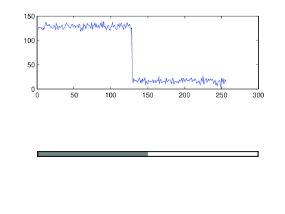
Figure 1: One dimensional, two classes.

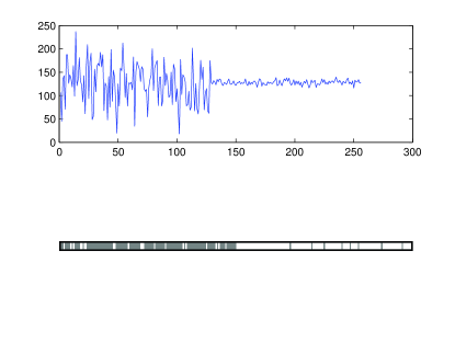
Figure 2: One dimensional, two classes.

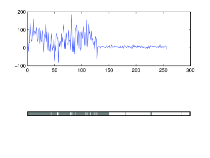
Figure 3: One dimensional, two classes.

In Fig. 4, we depict the result of the proposed algorithm for a two dimensional mixed signal of two classes, with one class having mean 200 and variance 400, and the other class having mean 5 and variance 400. The signal is shown in the left part of the figure. The classification result is shown in the right part of the figure. The false classification ratios are $1.93$% and $0.52$%. The size of the image is $32$ by $32$ pixels.

Figure 4: Two dimensional, two classes.

In summary, we find that the proposed classification algorithm is effective and robust. The algorithm has low computational complexity.

7 Conclusion

This paper proposes a blind classification algorithm for non-stationary signals, which can be modeled as mixtures of signals from several information sources. The proposed algorithm is based on data compression principles and relaxed continuous optimizations. We present theoretical discussions, which show that our algorithm is asymptotically optimal. Numerical results show that the proposed algorithm is effective, robust and has low computational complexity. The proposed algorithm can be used to solve various multimedia signal segmentation, analysis, and pattern recognition problems.

References

- [1] K. Azuma. Weighted sums of certain dependent random variables. Tohoku Mathematical Journal, 19(3):357–367, 1967.
- [2] W. Chen and C. Smith. Adaptive coding of monochrome and color images. IEEE Transactions on Communications, 25(11):1285–1292, November 1977.
- [3] T. cover and J. Thomas. Elements of Information Theory. John Wiley & Sons, 1991.
- [4] A. Dempster, N. Laird, and D. Rubin. Maximum likelihood from incomplete data via the em algorithm. Journal of the Royal Statistical Society, Series B, 39(1):1–38, 1977.
- [5] R. Duda, P. Hart, and D. Stork. Pattern Classification (2nd Edition). John Wiley & Sons, 2000.
- [6] S. Janson. On concentration of probability. Proceedings of Workshop on Probabilistic Combinatorics at the Paul Erdos Summer Research Center, Budapest, pages 289–301, 1998.
- [7] R. Joshi, H. Jafarkhani, J. Kasner, T. Fischer, N. Farvardin, M. Marcellin, and R. Bamberger. Comparison of different methods of classification in subband coding of images. IEEE Transactions on Image Processing, 6(11):1473–1486, November 1997.
- [8] X. Ma. Information theoretic analysis of the data compression based signal classification algorithm (working paper).
- [9] M. Sezgin and B. Sankur. Survey over image thresholding techniques and quantitative performance evaluation. Journal of Electronic Imaging, 13(1):146–165, January 2004.
- [10] U. Srinivasan, S. Pfeiffer, S. Nepal, M. Lee, L. Gu, and S. Barrass. A survey of mpeg-1 audio, video and semantic analysis techniques. Journal Multimedia Tools and Applications, 27(1):105–141, August 2005.
- [11] S. Theodoridis and K. Koutroumbas. Pattern Recognition (Third Edition). Academic Press, 2006.
- [12] Y.-T. Tse. Video coding using global/local motion compensation, classified subband coding, uniform threshold quantization and arithmetic coding (Ph.D. Thesis). University of California, Los Angeles, 1992.
- [13] A. Wachter and L. T. Biegler. On the implementation of a primal-dual interior point filter line search algorithm for large-scale nonlinear programming. Mathematical Programming, 106(1):25–27, May 2006.
- [14] J. Woods and S. O’Neil. Subband coding of images. IEEE Transactions on Acoustics, Speech, and Signal Processing, 34(5):1278–1288, October 1986.
- [15] Y. Yoo, A. Ortega, and B. Yu. Image subband coding using context-based classification and adaptive quantization. IEEE Transactions on Image Processing, 8(12):1702–1715, December 1999.