New approach to the Parton Distribution Functions: Self-Organizing Maps

Abstract:

We propose a Parton Distribution Function (PDF) fitting technique which is based on an interactive neural network algorithm using Self-Organizing Maps (SOMs). SOMs are visualization algorithms based on competitive learning among spatially-ordered neurons. Our SOMs are trained with stochastically generated PDF samples. On every optimization iteration the PDFs are clustered on the SOM according to a user-defined feature and the most promising candidates are selected as a seed for the subsequent iteration. Our main goal is thus to provide a fitting procedure that, at variance with the global analyses and standard neural network approaches, allows for an increased control of the systematic bias by enabling user interaction in the various stages of the fitting process.

1 Introduction

The cross sections for a number of hadronic reactions can be computed using perturbative Quantum Chromodynamics (pQCD) convoluting the perturbatively calculable hard scattering coefficients with the non perturbative Parton Distribution Functions (PDFs), that parametrize the large distance hadronic structure. The accuracy with which the theoretical predictions for observables of such reactions can be compared against the high precision experimental data thus depends, not only on the accuracy of the hard scattering part calculations, but also on the accuracy with which the PDFs are known.

Currently, the established method to obtain the PDFs, used by the major PDF collaborations (CTEQ [1] and references within, MRST [2], Alekhin [3], Zeus [4] and H1 [5]), is the global analysis supplemented with an error estimation using some kind of variant of the Hessian method (see e.g. [6] for details). This powerful combination allows for both extrapolation outside the kinematical range of the data and extension to multivariable cases, such as nuclear PDFs. However, there are uncertainties related to the method itself, that are difficult to quantify, but may turn out to have a large effect. The differences between the current global PDF sets indeed tend to be larger than the estimated uncertainties [7], and these differences again translate to the predictions for the LHC observables, such as Higgs [8] or $W^{\pm}$ and $Z$ production cross sections [1]. For details of PDF uncertainty studies see e.g. Refs. [9].

Another approach to the PDF fitting has recently been proposed by the NNPDF collaboration [10], who have replaced typical functional form ansatze used in global analyses with more complex standard neural network (NN) solutions, and the Hessian method with Monte Carlo (MC) sampling of the data. The NNPDF method circumvents many of the problems global analyses suffer, such as bias resulting from fixing a functional form and selecting a suitable tolerance $\Delta\chi^{2}$ needed in Hessian method, and it relies on genetic algorithm (GA) which works on a population of solutions for each MC replica of the data, thus having a lowered possibility of getting fixed in local minima. The estimated uncertainties for NNPDF fits are larger than those of global fits, possibly indicating that the global fit uncertainties may have been underestimated. The complexity of NN results, however, may also induce problems, especially when used in a purely automated fitting procedure. Since the effect of modifying individual NN parameters is unknown, the result may exhibit strange or unwanted behaviour in the extrapolation region, or in between the data points if the data is sparse. Implementation of information not given directly by the data, such as nonperturbative models, lattice calculations or knowledge from prior work in general, is also difficult in this approach.

The new PDF fitting method we have recently proposed in Ref. [11] relies on the use of Self-Organizing Maps (SOMs), a subtype of neural network. The idea of our method is to create means for introducing “Researcher Insight” instead of “Theoretical bias” by giving up a fully automated fitting procedure, and eventually to develop an interactive fitting program which would allow us to combine the best features of both the global analysis and the NNPDF approach.

2 Self-Organizing Maps

The SOM [12] is a visualization algorithm which attempts to represent all the available observations with optimal accuracy using a restricted set of models. SOM consists of nodes, map cells, which are all assigned spatial coordinates, and the topology of the map is determined by a chosen distance metric $M_{\mathrm{map}}$. Each cell $i$ contains a map vector $V_{i}$, that is isomorphic to the data samples used for training of the neural network. For a simple 2-dimensional rectangular lattice, our choice for the SOM shape, a natural choice for the topology is $L_{1}(x,y)=\sum_{i=1}^{2}|x_{i}-y_{i}|$.

The implementation of SOMs proceeds in three stages: 1) initialization of the SOM (see Fig. 1), 2) training of the SOM (Fig. 1) and 3) associating the data samples with a trained map, i.e. clustering. For the details of the SOM implementation, see [11].

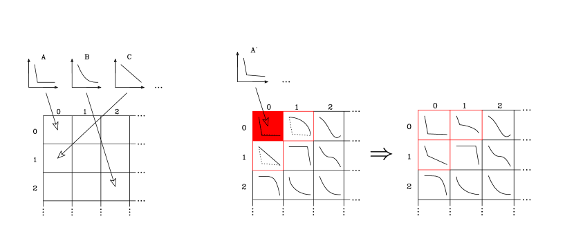
Figure 1: Left: SOM initialization, Right: SOM training.

In the end of the training stage, cells that are topologically close to each other have map vectors which are most similar to each other (according to a chosen similarity metric $M_{\rm data}$) compared to all the other map vectors. In the matching phase the actual data is matched against the map vectors of the trained map, and thus get distributed on the map according to the feature that was used as the similarity criterion. Clusters now emerge as a result of unsupervised learning. This local similarity property is the feature that makes SOM suitable for visualization purposes, thus facilitating user interaction with the data. Since each map vector now represent a class of similar objects, the SOM is an ideal tool to visualize high-dimensional data, by projecting it onto a low-dimensional map clustered according to some desired similar feature.

In our work we used the so-called batch-version of the training, in which all the training data samples are matched against the map vectors before the training begins. The map vectors are then averaged with all the training samples within the neighbourhood radius simultaneously. The procedure is repeated $N_{\mathrm{step}}$ (free parameter to choose) times such that in every training step the same set of training data samples is associated with the evolving map The benefit of the batch training compared to the incremental training, shown in Fig. 1, is that the training is independent of the order in which the training samples are introduced on the map.

3 ENVPDF algorithm

The aim of our approach is to both i) to be able to study the properties of the PDFs in a model independent way and yet ii) to be able to implement knowledge from the prior works on PDFs, and ultimately iii) to be able to guide the fitting procedure interactively with the help of the SOM properties.

To accomplish this, we choose, at variance with the “conventional” PDFs sets or NNPDFs, to give up the functional form for the PDFs and rather to rely on purely stochastical methods in generating the initial and training PDF samples. Our choice is a GA-type analysis, in which our parameters are the values of PDFs at the initial scale for each flavour at each value of $x$ where the experimental data exist. To obtain control over the shape of the PDFs we use some of the existing distributions to establish an initial range, or envelope, within which we sample the candidate PDF values.

For now we concentrate on DIS structure function data from H1 [13], BCDMS [14] and Zeus [15], which we use without additional kinematical cuts or normalization factors. The parameters for the DGLAP scale evolution were chosen to be those of CTEQ6 (CTEQ6L1 for lowest order (LO)) [16], the initial scale being $Q_{0}=1.3$ GeV. In next-to-leading order (NLO) case the evolution code was taken from [17] (QCDNUM17 beta release).

We use CTEQ6 [16], CTEQ5 [18], MRST02 [2, 19], Alekhin [3] and GRV98 [20] PDF sets as our init PDFs. We construct our initial PDF generator first to, for each flavour separately, select randomly either the range $[0.5,1]$, $[1.0,1.5]$ or $[0.75,1.25]$ times any of the init PDF set. Next the initial generators generate values for each $x_{\rm data}$ ( To ensure a reasonable large-$x$ behaviour for the PDFs, we also generate with the same method values for them in a few $x$-points outside the range of the experimental data. For simplicity we also require the gluons to be positive in NLO.) using uniform, instead of Gaussian, distribution around the init PDFs, thus reducing direct bias from them. Gaussian smoothing is applied to the resulting set of points, and the flavours combined to form a PDF set such that the curves are linearly interpolated from the discrete set of generated points, and scaled to conserve momentum, baryon number and charge. In this study we accept the $<$few% normalization error which results from the fact that our x-range is not $x=[0,1]$, but $x=[{\rm min}(x_{\rm data}),1]$. We call these type of PDF sets database PDFs.

For a $N\times N$ SOM we choose the size of the database to be $4N^{2}$. We randomly initialize the map with $N$ database PDFs sets, such that each map vector $V_{i}$ consists of the PDF set itself, and of the observables $F_{2}^{p}(x,Q_{0}^{2})$ derived from it, and train the map with $N_{\mathrm{step}}$ batch-training steps. In order to obtain a reasonable selection of PDFs to start with, we reject candidates which have $\chi^{2}/N>10$. We choose the similarity criterion to be the similarity of observables $F_{2}^{p}(x,Q^{2})$ with $M_{\mathrm{data}}=L_{1}$. The similarity is tested at every $x_{\rm data}$-values both at the initial scale and at all the evolved scales where experimental data exist. On every training step, after the matching, all the observables (PDFs) of the map vectors get averaged with the observables (PDFs, flavor by flavor) matched within the neighbourhood. The resulting new averaged map vector PDFs are rescaled again to obey the sumrules. We call these type of PDF sets map PDFs. The map PDFs are evolved and the observables at every experimental data scale are computed and compared for similarity with the observables from the training PDFs. After the training we have a map with $N$ map PDFs and the same $4N^{2}$ database PDF sets we used to train the map. This is the end of the first optimization iteration.

During the later iterations we proceed as follows: At the end of each iteration we pick from the trained SOM $2N$ best PDFs as the init PDFs. These init PDFs are introduced into the training set alongside with the database PDFs, which are now constructed using each of the init PDFs in turn as a center for a Gaussian random number generator, which assigns for all the flavours for each $x$ a value around that same init PDF such that $1-\sigma$ of the generator is given by the spread of the best PDFs in the topologically nearest neighbouring cells. The object of these generators is thus to refine a good candidate PDF found in the previous iteration by jittering its values within a range determined by the shape of other good candidate PDFs from the previous iteration. The generated PDFs are then smoothed and scaled to obey the sumrules. Sets with $\chi^{2}/N>10$ are always rejected. It is important to preserve the variety of the PDF shapes on the map, so we also keep $N_{\rm orig}$ copies of the first iteration generators in our generator mix. Since the best PDF candidates from the previous iteration are matched on this new map as an unmodified init PDF, it is guaranteed that the $\chi^{2}/N$ as a function of the iteration either decreases or remains the same. We keep repeating the iterations until the $\chi^{2}/N$ saturates.

The best $\chi^{2}/N$ values of the original init PDFs are 1.67 for LO (CTEQ6) and 1.89 for NLO (MRST02), and Table 1 lists results from a variety of ENVPDF runs. The results do not seem to be very sensitive to the number of SOM training steps, $N_{\rm step}$, but are highly sensitive to the number of first iteration generators used in subsequent iterations. Although the generators can now in principle produce an infinite number of different PDFs, the algorithm would not be able to radically change the shape of the database PDFs without introducing a random element on the map. Setting $N_{\rm orig}>0$ provides, through map PDFs, that element, and keeps the algorithm from getting fixed to a local minimum.

SOM	$N_{\rm step}$	$N_{\rm orig}$	LO $\chi^{2}/N$	NLO $\chi^{2}/N$
5x5	5	2	1.04	1.08
5x5	10	2	1.10	-
5x5	20	2	1.10	-
5x5	30	2	1.10	-
5x5	40	2	1.08	-
5x5	5	0	1.41	-
15x15	5	6	1.00	1.07

Table 1: $\chi^{2}/N$ for variety of ENVPDF runs against all the datasets (H1, ZEUS, BCDMS, N=709).

Due to the stochastical nature of the ENVPDF algorithm, we may well study the combined results from several separate runs. It is especially important to verify the stability of our results, to show that the results are indeed reproducible instead of lucky coincidences. Left panel of Fig. 2 presents the best NLO results, and the combined $\chi^{2}/N\leq 1.2$ spreads of the PDFs from any iteration, for 10 repeated $5\times 5$, $N_{\rm step}=5$ runs at the initial scale. The average $\chi^{2}/N$ and the standard deviation $\sigma$ for these runs are 1.122 and 0.029, corresponding to $\Delta\chi^{2}\sim 20$. The right panel of the same Fig. 2 shows the 10 best result curves and the $\chi^{2}/N\leq 1.2$ spreads evolved up to $Q=3.0$ GeV. Since we have only used DIS data in this study, we are only able to explore the small-$x$ uncertainty for now, and expectedly, the small-$x$ gluons obtain the largest uncertainty for all the cases we studied.

Clearly the seemingly large difference between the small-$x$ gluon results at the initial scale is not statistically significant, but gets smoothed out during the course of the QCD evolution. The evolved curves also preserve the initially set baryon number scaling within $~{}0.5\%$ and momentum sumrule within $~{}1.5\%$ accuracy. Thus the initial scale wiggliness of the PDFs is mainly only a residual effect from our method of generating them and not linked to the overtraining of the SOM.

Therefore our simple method of producing the candidate PDFs by jittering random numbers inside a predetermined envelope is surprisingly stable when used together with a complicated PDF processing that SOMs provide. Remarkably then, even a single SOM run can provide a quick uncertainty estimate for a chosen $\Delta\chi^{2}$ without performing a separate error analysis.

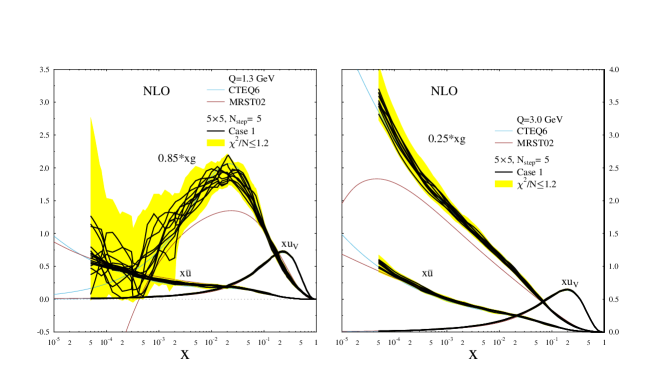
Figure 2: NLO ENVPDF best results and the $\chi^{2}/N\leq 1.2$ spreads of results from 10 separate runs.

4 Future of the SOMPDFs

So far we have shown a relatively straightforward method of obtaining stochastically generated, parameter-free, PDFs, with an uncertainty estimate for a desired $\Delta\chi^{2}$. However, the proposed method can be extended much further than that. What ultimately sets the SOM method apart from the standard global analyses or NNPDF method are the clustering and visualization possibilities that it offers. Instead of setting $M_{\mathrm{data}}=L_{1}$ and clustering according to the similarity of the observables, it is possible to set the clustering criteria to be anything that can be mathematically quantified, e.g. the shape of the gluons or the large-$x$ behaviour of the PDFs. The desired feature of the PDFs can then be projected out from the SOM. Moreover, by combining the method with an interactive graphic user interface (GUI), it would be possible to change and control the shape and the width of the envelope as the minimization proceeds, to guide the process by applying researcher insight at various stages of the process, and the uncertainty band produced by the SOM could further help the user to make decisions about the next steps of the minimization. With GUI it would be e.g. possible to set the generators to sample a vector consisting of PDF parameters, instead of values of PDFs in each value of $x$ of the data. That would lead to smooth, continuous type of solutions, either along the lines of global analyses, or NNPDFs using $N$ SOMs for $N$ Monte-Carlo sampled replicas of the data. For such a method, all the existing error estimates, besides an uncertainty band produced by the map, would be applicable as well. Since the solution would be required to stay within an envelope of selected width and shape, no restrictions for the parameters themselves would be required, and it would be possible to e.g. to constrain the extrapolation of the NN generated PDFs outside the $x$-range of the data without explicitly introducing terms to ensure the correct small- and large-$x$ behaviour as in NNPDF method. The selection of the best PDF candidates for the subsequent iteration could then be made based on the user’s preferences instead of solely based on the $\chi^{2}/N$. That kind of method in turn could be extended to more complex hadronic matrix elements, such as the ones defining the GPDs, which are natural candidates for future studies of cases where the experimental data are not numerous enough to allow for a model independent fitting, and the guidance and intuition of the user is therefore irreplaceable. The possibilities of such a method are widely unexplored.

References

- [1] P. M. Nadolsky et al., arXiv:0802.0007 [hep-ph].
- [2] A. D. Martin, R. G. Roberts, W. J. Stirling and R. S. Thorne, Eur. Phys. J. C 23 (2002) 73 [arXiv:hep-ph/0110215]; A. D. Martin, R. G. Roberts, W. J. Stirling and R. S. Thorne, Phys. Lett. B 604 (2004) 61 [arXiv:hep-ph/0410230]; A. D. Martin, W. J. Stirling, R. S. Thorne and G. Watt, Phys. Lett. B 652 (2007) 292 [arXiv:0706.0459 [hep-ph]].
- [3] S. Alekhin, Phys. Rev. D 68 (2003) 014002 [arXiv:hep-ph/0211096]; S. Alekhin, K. Melnikov and F. Petriello, Phys. Rev. D 74 (2006) 054033 [arXiv:hep-ph/0606237].
- [4] S. Chekanov et al. [ZEUS Collaboration], Eur. Phys. J. C 42 (2005) 1 [arXiv:hep-ph/0503274].
- [5] C. Adloff et al. [H1 Collaboration], Eur. Phys. J. C 30 (2003) 1 [arXiv:hep-ex/0304003].
- [6] J. Pumplin et al., Phys. Rev. D 65 (2002) 014013 [arXiv:hep-ph/0101032].
- [7] J. Pumplin, AIP Conf. Proc. 792, 50 (2005) [arXiv:hep-ph/0507093].
- [8] A. Djouadi and S. Ferrag, Phys. Lett. B 586 (2004) 345 [arXiv:hep-ph/0310209].
- [9] A. D. Martin, R. G. Roberts, W. J. Stirling and R. S. Thorne, Eur. Phys. J. C 35 (2004) 325 [arXiv:hep-ph/0308087]; A. D. Martin, R. G. Roberts, W. J. Stirling and R. S. Thorne, Eur. Phys. J. C 28 (2003) 455 [arXiv:hep-ph/0211080].
- [10] M. Ubiali, arXiv:0809.3716 [hep-ph]; R. D. Ball et al., arXiv:0808.1231 [hep-ph].
- [11] J. Carnahan, H. Honkanen, S. Liuti, Y. Loitiere and P. R. Reynolds, arXiv:0810.2598 [hep-ph].
- [12] T. Kohonen, Self-organizing Maps, Third Edition, Springer (2001); http://www.cis.hut.fi/projects/somtoolbox
- [13] C. Adloff et al. [H1 Collaboration], Eur. Phys. J. C 21 (2001) 33 [arXiv:hep-ex/0012053].
- [14] A. C. Benvenuti et al. [BCDMS Collaboration], Phys. Lett. B 223 (1989) 485; A. C. Benvenuti et al. [BCDMS Collaboration], Phys. Lett. B 237 (1990) 592.
- [15] S. Chekanov et al. [ZEUS Collaboration], Eur. Phys. J. C 21 (2001) 443 [arXiv:hep-ex/0105090].
- [16] J. Pumplin, D. R. Stump, J. Huston, H. L. Lai, P. Nadolsky and W. K. Tung, JHEP 0207 (2002) 012 [arXiv:hep-ph/0201195].
- [17] http://www.nikhef.nl/ h24/qcdnum/
- [18] H. L. Lai et al. [CTEQ Collaboration], Eur. Phys. J. C 12 (2000) 375 [arXiv:hep-ph/9903282].
- [19] A. D. Martin, R. G. Roberts, W. J. Stirling and R. S. Thorne, Phys. Lett. B 531 (2002) 216 [arXiv:hep-ph/0201127].
- [20] M. Gluck, E. Reya and A. Vogt, Eur. Phys. J. C 5 (1998) 461 [arXiv:hep-ph/9806404].