Doppler maps and surface differential rotation of EI Eri from the MUSICOS 1998 observations

Abstract

We present time-series Doppler images of the rapidly-rotating active binary star EI Eri from spectroscopic observations collected during the MUSICOS multi-site campaign in 1998, since the critical rotation period of 1.947 days makes it impossible to obtain time-resolved images from a single site. From the surface reconstructions a weak solar-type differential rotation, as well as a tiny poleward meridional flow are measured.

1 Introduction

Due to the fast disperse of high resolution spectroscopic observational facilities, surface differential rotation (hereafter DR) measurements has become achievable for stars of different types, giving a useful contribution for developing solar and stellar dynamo theory. Indirect imaging techniques, such as Doppler imaging can help in extending this input knowledge by tracing the positions of different spots/magnetic features on consecutive surface maps. The method of cross-correlating consecutive Doppler images to follow the time evolution of the spots and to derive surface DR was demonstrated for the first time for AB Dor 1997MNRAS.291….1D , and it has been used extensively thenceforth. Unfortunately, rapid spot changes can fade out the correlation pattern of the DR. On the other hand, averaging many cross-correlation maps can overwhelm the masking effect of random-like short-term spot changes 2004A&A…417.1047K .

In this paper we present time-series Doppler images for the rapidly rotating active binary star EI Eridani (HD 26337). From the consecutive surface maps we measure surface DR. Since the rotation period of the star is nearly 2 days, data with sufficient phase coverage for a Doppler image can only be collected over about 15 days from a single observing site. Thus, the reconstructed surface map is necessarily time-averaged, which makes DR measurements unfeasible. To avoid this problem, in our study we use a set of high resolution spectra collected in the fifth MUSICOS (MUlti-SIte COntinuous Spectroscopy) campaign in 1998, which allows to derive time-resolved surface maps.

2 Observations

Figure 1: Observing sites involved in the MUSICOS 98 campaign

The fifth MUSICOS campaign took place from November 22 to December 11, 1998. It involved eight northern and southern sites and ten telescopes of 2m class, mostly equipped with cross-dispersed echelle spectrographs. Fig. 1 shows the distribution of the participating observatories. From the total of 122 high-resolution spectra obtained in the campaign for EI Eridani, 81 spectra were suitable for the purposes of Doppler imaging. Spectroscopic observations are supported by simultaneous photometry carried out with the Wolfgang-Amadeus twin Automatic Photoelectric Telescope (APT) at Fairborn Observatory, Arizona (kgs:boyd97, ). Phases of all line profiles are computed using the ephemeris $HJD=2\,448\,054.7130+1.9472287\times E$ wasi03 .

3 Time-series Doppler imaging

From the chronologically listed 81 spectra obtained during 20 days, we form 52 subsets with 30-30 spectra. Each subset is formed from the preceeding one by dropping the spectrum from the beginning of the list and adding the subsequent one to the end. From these overlapping subsets we compute 52 surface maps using our Doppler imaging code TempMap 1989A&A…208..179R . As astrophysical input we use the data listed in Table 1 taken from paper2 . The resulted Doppler maps confirm the existence of a stable polar spot changing slightly in size and shape, while low latitute spots are found to be short lived. Independent inversions for the CaI-6439 and for the FeI-6411 mapping lines are in good agreement, as seen in the corresponding example image pair in Fig. 2.

Parameter	Value
$P_{\rm phot}=P_{\rm rot}$	1.9472324 d
T${}_{\rm 0,phot}=$T0,rot	2448054.7109 d
$\gamma$	21.64 km/s
K1	26.83 km/s
$e$ (eccentricity)	0 (adopted)
$T_{\rm phot}$	5500 K
$T_{\rm max}$	6000 K
$v\sin i$	51.0 km/s
Inclination $i$	56.0∘
$\log g$	3.5
Microturbulence $\xi$	2.0 km/s
Macroturbulence $\zeta_{\rm r}=\zeta_{\rm t}$	4.0 km/s
$\log[Ca]$ abundance	$-6.3$ (0.6 dex below solar)
$\log[Fe]$ abundance	$-5.5$ (1.1 dex below solar)

Table 1: Stellar parameters of EI Eri

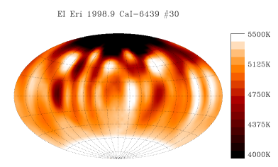
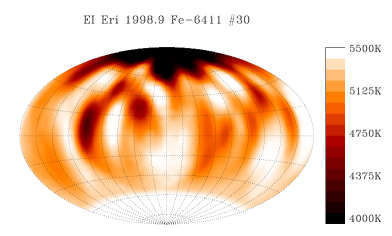
Figure 2: Simultaneous example image reconstructions from the time-series for the CaI-6439 (top) and for the FeI-6411 (bottom) mapping lines

4 Differential rotation and meridional flow

For measuring surface DR we apply the technique called ACCORD (Average Cross-CORrelation of time-series Doppler images) introduced for the time-series Doppler maps of LQ Hya in 2004A&A…417.1047K , and applied more recently to $\sigma$ Gem kovarietalsgem07 and to $\zeta$ And kovari:bartus:wasi07 . The 52 time-series Doppler images are coupled in order to obtain 22 pairs of non-overlapping, consecutive Doppler maps. These pairs are cross-correlated and the resulting correlation function (ccf) maps are averaged. On the resulting average ccf map, we fit the correlation peak for each latitudinal strip with a Gaussian profile. The Gaussian peaks per latitude strips then represent the DR pattern and can thus be fitted with a standard solar-like quadratic DR law. The best fit DR function for the combined Ca+Fe ccf map in the left panel of Fig. 3 indicates a DR parameter $\alpha=\Delta\Omega/\Omega$ of 0.037, about one-sixth of the value measured on the Sun.

An average meridional flow can be quantified by using ACCORD, since latitudinal motion of spots can be analysed by cross-correlating the corresponding longitude strips along the meridian circles. For this we use only the hemisphere of the visible pole where Doppler imaging is more reliable. The correlation maxima for each longitudinal strip are fitted with a Gaussian and the resulting peaks represent the best correlating latitudinal shifts. For a detailed description of the method see kovarietalsgem07 . The latitudinal correlation pattern plotted in the right panel of Fig. 3 can be converted into an average poleward velocity field of less than 100 m/s. For further details see our forthcoming paper forthcom .

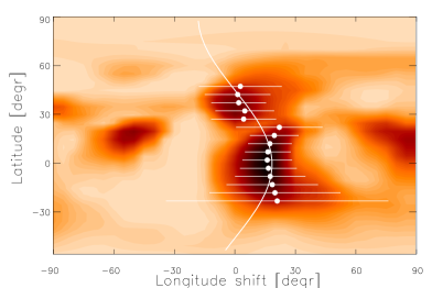
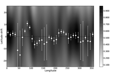
Figure 3: Resulting average ccf map with the best fit DR law (left) and the latitudinal ccf map (right)

References

- (1) J.-F. Donati, and A. Collier Cameron, MNRAS 291, 1 (1997).
- (2) Z. Kővári, K. G. Strassmeier, T. Granzer, M. Weber, K. Oláh, and J. B. Rice, A&A 417, 1047 (2004).
- (3) K. G. Strassmeier, L. J. Boyd, D. H. Epand, and T. Granzer, PASP 109, 697 (1997).
- (4) A. Washuettl, K. G. Strassmeier, B. Foing, and MUSICOS98 Team, “MUSICOS Observations of the Chromospherically Active Binary Star EI Eridani,” in 12th Cambridge Workshop on Cool Stars, Stellar Systems, and the Sun, eds. A. Brown, G.M. Harper, and T.R. Ayres, (University of Colorado), 2003, p. 1008.
- (5) J. B. Rice, W. H. Wehlau, and V. L. Khokhlova, A&A 208, 179 (1989).
- (6) A. Washuettl, K. G. Strassmeier, and M. Weber, Astron. Nachr. (2008), submitted.
- (7) Z. Kővári, J. Bartus, K. G. Strassmeier, K. Vida, M. Švanda, and K. Oláh, A&A 474, 165 (2007).
- (8) Z. Kővári, J. Bartus, K. G. Strassmeier, K. Oláh, M. Weber, J. B. Rice, and A. Washuettl, A&A 463, 1071 (2007).
- (9) A. Washuettl, Z. Kővári, B. H. Foing, K. Oláh, M. Weber, D. García-Alvarez, O. J., Y. Unruh, and MUSICOS 98 Team, A&A (2008), submitted.