Quasi-chemical theory with a soft cutoff

Abstract

In view of the wide success of molecular quasi-chemical theory of liquids, this paper develops the soft-cutoff version of that theory. This development has important practical consequences in the common cases that the packing contribution dominates the solvation free energy of realistically-modeled molecules because treatment of hard-core interactions usually requires special purpose simulation methods. In contrast, treatment of smooth repulsive interactions is typically straightforward on the basis of widely available software. This development also shows how fluids composed of molecules with smooth repulsive interactions can be treated analogously to the molecular-field theory of the hard-sphere fluid. In the treatment of liquid water, quasi-chemical theory with soft-cutoff conditioning doesn’t change the fundamental convergence characteristics of the theory using hard-cutoff conditioning. In fact, hard cutoffs are found here to work better than softer ones.

I Introduction

Recent developments of quasi-chemical theory constitute a fresh attack on the theory of solutions from a molecular scale, a point that has been noted before.PrattLR:Quatst ; Paulaitis:02 ; beck2006 ; CPMS Quasi-chemical theory provides a natural organization for calculations of ion-water chemical interactions in the treatment of ion hydration free energies.Rempe:JACS:2000 ; AsthagiriD:Hydsaf ; CPMS A remarkably natural quasi-chemical theory for the statistical thermodynamics of liquid watershah:144508 can be implemented on the basis of the massive data sets of molecular simulations and provides a realistic direct evaluation of the entropy of that liquid. For non-polar solutes dissolved in liquid water, quasi-chemical theory avoids physical assumptions of the van der Waals (perturbative) type that are otherwise common, and thus resolves questions centering on reference system assumptions.AsthagiriD.:NonWth ; Asthagiri:2008p1418 As originally developed with a sharp cutoff to spatially define the inner shell, quasi-chemical theory implemented as a molecule-field theory for the hard-sphere fluid provides an equation of state as accurate as the most accurate previous theory.PrattLawrenceR.:Selmft

This quasi-chemical theory can be expressed entirely as statistical modeling of the distribution $P(\varepsilon)$ of energies $\varepsilon$ binding a distinguished molecule to the medium. A goal is to discriminate effects of close, or inner-shell, neighbors of that molecule from the effects of the more distant material. This is done by formulating a statistical condition to identify inner-shell molecules. We will express our condition with $\chi$, a function indicating that the inner shell is empty when $\chi=1$. $\chi$ has been assumed to be either 0 or 1, sharply changing between those possibilities. We then direct attention to the conditional probability $P(\varepsilon|\chi=1)$ in order to define an outer-shell contribution, and then further use chemical concepts to evaluate the remainder associated with occupancy of the inner-shell.

This quasi-chemical theory with sharp- or hard-cutoff conditioning works satisfactorily both for the free energy of liquid watershah:144508 and for the hydration free energy of CF₄(aq).AsthagiriD.:NonWth In the latter case, the theory generates a result similar to a van der Waals theory without requiring those assumptions in advance. A prominent contribution to that result is a hard-core or packing contribution associated with the sharp $\chi=1$ condition. On an intuitive basis, it is widely asked whether a more natural packing contribution might be based upon smooth repulsive interactions. In the contrasting case of liquid water, more aggressive conditioning is required, and the packing contribution clearly does not have the logical status of a contribution of repulsive-force reference interaction considered to be similar to actual intermolecular interactions. The present work is designed to clarify these contrasting points.

We anticipate the results below by noting here that the theory for the soft-cutoff conditioning can be developed in straightforward analogy with that for hard-cutoff conditioning. This development has important practical consequences because a packing contribution frequently dominates the solvation free energy of realistically-modeled molecules but treatment of hard-core interactions associated with a hard cutoff usually requires special purpose calculations. Examples of the special considerations that apply to simulation of liquids of hard-core-model polyatomic molecules can be found in the references.Stratt:1981p3179 ; Smith:1997p3228 In contrast, treatments of smooth repulsive interactions are typically straightforward on the basis of widely available software. The present development implies also that fluids composed of molecules with smooth repulsive interactions can be treated by analogy with the molecular-field theory of the hard-sphere fluid.PrattLawrenceR.:Selmft

In a case such as CF₄(aq) where only minimal conditioning is required,AsthagiriD.:NonWth we propose below a soft cutoff that should reduce the variance of estimates of the required contributions. In the case of liquid water where aggressive conditioning is required,shah:144508 we can systematically vary the softness of the cutoff defining the inner shell, and attempt to learn what works best.

II Theory

Quasi-chemical theory with sharp- or hard-cutoff conditioning, which we aim to generalize, can be expressed as

$$\beta\mu^{\mathrm{ex}}=-\ln\left<\left<\chi\right>\right>_{0}+\ln\left<\chi\right>+\ln\int\mathrm{e}^{\beta\varepsilon}P(\varepsilon|\chi=1)\mathrm{d}\varepsilon~{},$$ (1a)

$$\beta\mu^{\mathrm{ex}}\approx-\ln\left<\left<\chi\right>\right>_{0}+\ln\left<\chi\right>\\ +\beta\left<\varepsilon|\chi=1\right>+\frac{\beta^{2}}{2}\left<\delta\varepsilon^{2}|\chi=1\right>~{}.$$ (1b)

The notation $\left<\left<\ldots\right>\right>_{0}$ indicates the average over the thermal motion of the system and the solute with no interaction between them, thus the subscript 0. $\chi$ is an indicator function and $\chi=1$ defines our condition. As an example, for the application to liquid water $\chi=1$ when there are no O-atoms of bath molecules within a radius $\lambda$ from the O-atom of a distinguished water molecule. Then $\chi=0$ if any solvent molecule is present in that inner-shell. The conditional averages indicate that statistics are collected only when $\chi=1$. Significant conditioning produces slightly sub-gaussian binding energy probability densities $P(\varepsilon|\chi=1)$. Slight sub-gaussian behavior leads to errors of 1 kcal/mol in the excess chemical potentials calculated with Eq. (1b).shah:144508 ; Crete2008 Nevertheless, Eq. (1b) adopts the gaussian approximation.

The generalization that we seek can be economically identified on the basis of a few primitive relations. The first is the rule of averages CPMS

$$\left<F\right>=\frac{\left\langle\left\langle\mathrm{e}^{-\beta\Delta U}F\right\rangle\right\rangle_{0}}{\left\langle\left\langle\mathrm{e}^{-\beta\Delta U}\right\rangle\right\rangle_{0}}=\mathrm{e}^{\beta\mu^{\mathrm{ex}}}\left\langle\left\langle\mathrm{e}^{-\beta\Delta U}F\right\rangle\right\rangle_{0}~{}.$$ (2)

Then,

$$\left<\mathrm{e}^{\beta\Delta U}\chi\right>=\mathrm{e}^{\beta\mu^{\mathrm{ex}}}\left\langle\left\langle\chi\right\rangle\right\rangle_{0}$$ (3)

is an example of specific utility for our argument. For an indicator function $\chi$ we have in addition

$$\left<G\chi\right>=\left<G|\chi=1\right>\left<\chi\right>~{},$$ (4)

and $\left<\chi\right>$ is a probability. Collecting these relations yields

$$\mathrm{e}^{\beta\mu^{\mathrm{ex}}}=\left<\mathrm{e}^{\beta\Delta U}|\chi=1\right>\times\left(\frac{\left<\chi\right>}{\left<\left\langle\chi\right\rangle\right>_{0}}\right)~{},$$ (5)

or Eq. (1a) after evaluating the logarithm. For a sharp cutoff case, this is obtained directly from the standard thermodynamic difference formula.shah:144508 ; Crete2008 Beyond traditional statistical thermodynamics, however, this formula only depends on the fact that $\chi$ is an indicator function.

We obtain soft-cutoff conditioning by designing an indicator function which categorizes a solvent molecule at a particular configuration to be either in or out of the inner shell according to a statistical rule. For example, let the designated or solute molecule be at a fixed position, and consider the $i^{th}$ solvent molecule again at a definite configuration denoted by $\mathcal{R}_{i}$. We take $0\leq b(\mathcal{R}_{i})\leq 1$ to be the probability that the $i^{th}$ solvent molecule is in, independent of any other characteristic. [For the cases considered above $b(\mathcal{R}_{i})$ only depends on the three-dimensional position of the O (oxygen) atom of the $i^{th}$ water molecule.] For each configuration, we could then sample $b(\mathcal{R}_{i})$ for each solvent molecule, and thereby identify each solvent molecule as either in or out. Exhaustive in-out sampling at a fixed configuration produces

$$\bar{\chi}=\prod_{j}(1-b(\mathcal{R}_{j}))$$ (6)

as a sampling-averaged indicator function. The formula specifically indicating a soft-cutoff is then

$$\mathrm{e}^{\beta\mu^{\mathrm{ex}}}=\left<\mathrm{e}^{\beta\Delta U}|\chi=1\right>\times\left(\frac{\left<\bar{\chi}\right>}{\left<\left\langle\bar{\chi}\right\rangle\right>_{0}}\right)~{}.$$ (7)

The hard-cutoff theory is recovered if step functions are chosen for the $b(\mathcal{R}_{i})$.

It is interesting to note that Eq. (3) is specialization of

$$\mathrm{e}^{\beta\mu^{\mathrm{ex}}}=\frac{\left<\mathrm{e}^{\beta\Delta U}W\right>}{\left<\left\langle W\right\rangle\right>_{0}}~{},$$ (8)

to the case that $W=\bar{\chi}$ is an indicator function. BennettBENNETTCH:Effefe has studied such forms without the restriction that $W$ be an indicator function, and found $W\propto(1+z\mathrm{e}^{\beta\Delta U})^{-1}$ to be statistically optimal with a particular value of $z$. In contrast, our goal is the dis-entanglement of the effects of longer-ranged intermolecular interactions from packing and chemical contributions, so we do not follow Bennett’s results here. A potential advantage of Eq. (7) is that $\left<\bar{\chi}\right>$ is an occupancy probability and therefore can be modeled on a pattern of chemical equilibria, as we elaborate below.

Nevertheless, if minimal conditioning is all that is required, then a straightforward suggestion for choice of the indicator function is $\bar{\chi}=\exp\left(-\beta u_{0}\right)$ for a smooth repulsive molecular-pair interaction, $u_{0}$, that matches $\Delta U$ at short range. In view of Eq. (8), this choice would reduce the variance of the numerator of Eq. (7). Then the denominator is $\left<\left\langle\bar{\chi}\right\rangle\right>_{0}=\exp\left(-\beta\mu^{\mathrm{ex}}_{0}\right)$.

Chemical interpretation

A general derivation of quasi-chemical theory Beck:2006 can be based upon an inclusion-exclusion development initiated from the tautology

$$1=\prod_{j}\left[b(\mathcal{R}_{j})+(1-b(\mathcal{R}_{j}))\right]~{}.$$ (9)

When included within the averaging brackets that yield the chemical potential, Eq. 9 leads to the general development Beck:2006

$$\mathrm{e}^{-\beta\mu_{\alpha}^{\mathrm{ex}}}=\left({1+\sum\limits_{n\geq 1}{K_{n}\rho^{n}}}\right)\times\left\langle{\left\langle\mathrm{e}^{-\beta\Delta U_{\alpha}}\bar{\chi}\right\rangle}\right\rangle_{0}~{}.$$ (10)

Since

$$\frac{\left\langle\left\langle\mathrm{e}^{-\beta\Delta U_{\alpha}}\bar{\chi}\right\rangle\right\rangle_{0}}{\left\langle\left\langle\mathrm{e}^{-\beta\Delta U_{\alpha}}\right\rangle\right\rangle_{0}}=\left\langle\bar{\chi}\right\rangle~{},$$ (11)

Eq. (10) implies

$$\left\langle\bar{\chi}\right\rangle=\frac{1}{{1+\sum\limits_{n\geq 1}{K_{n}\rho^{n}}}}~{}.$$ (12)

The $K_{n}$’s involve the cutoff function in a natural way.Beck:2006 Together with

$$p(n)=\left\langle{N\choose n}\left[\prod\limits_{j=1}^{j=n}b(\mathcal{R}_{j})\right]\left[\prod\limits_{k=n+1}^{k=N}\left(1-b(\mathcal{R}_{k})\right)\right]\right\rangle,$$ (13)

$K_{n}\rho^{n}$ is the ratio of the probability that the distinguished species has $n$ ligands to the probability that it has zero (0) ligands

$$\frac{p(n)}{p(0)}=K_{n}\rho^{n}~{}.$$ (14)

This is naturally interpreted on the basis of the chemical equilibrium

$$\mathrm{W}^{*}+n\mathrm{W}\leftrightharpoons\mathrm{W^{*}W}_{n}$$ (15)

where $\mathrm{W^{*}}$ denotes a water molecule with zero (0) ligands and $\mathrm{W^{*}W}_{n}$ denotes that water molecule with $n$ ligands occupying the inner shell. Given Eq. (12), the probability that the distinguished molecule has zero (0) ligands is $\left\langle\bar{\chi}\right\rangle$. This establishes the thermodynamic significance of that normalization factor. These interpretations are straightforward for the sharp-cutoff case. If the probabilities of Eq. (14) are given by a Poisson distribution, then $K_{n}=v^{n}/n!$ with $v$ the volume of the stencil. For a specified function $b(\mathcal{R}_{i})$, $p(n)$ and $K_{n}$ can be observed in conventional simulations where the full physical solute-solvent interactions are expressed.

These analogies go further. For example, consider the packing contribution $\left\langle{\left\langle\bar{\chi}\right\rangle}\right\rangle_{0}$,Beck:2006 and apply Eq. (10) to the case $\Delta U_{\alpha}$ = 0. This yields

$$1=\left({1+\sum\limits_{n\geq 1}{\tilde{K}_{n}\rho^{n}}}\right)\times\left\langle{\left\langle\bar{\chi}\right\rangle}\right\rangle_{0}~{},$$ (16)

or

$$\left\langle{\left\langle\bar{\chi}\right\rangle}\right\rangle_{0}=\frac{1}{\left({1+\sum\limits_{n\geq 1}{\tilde{K}_{n}\rho^{n}}}\right)},$$ (17)

with

$$\frac{\tilde{p}(n)}{\tilde{p}(0)}=\tilde{K}_{n}\rho^{n}~{}.$$ (18)

Here the tildes indicate quantities observed without the solute physically present, but with a soft stencil defined by the indicator function $\bar{\chi}$. Specifically

$$\tilde{p}(n)=\\ \left\langle\left\langle{N\choose n}\left[\prod\limits_{j=1}^{j=n}b(\mathcal{R}_{j})\right]\left[\prod\limits_{k=n+1}^{k=N}\left(1-b(\mathcal{R}_{k})\right)\right]\right\rangle\right\rangle_{0},$$ (19)

i.e., Eq. (13) for the present uncoupled case. Fig. 1 gives example results of $\tilde{p}\left(n\right)$ for liquid water, and shows that soft-cutoff conditioning produces integer-referenced probabilities.

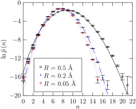
Figure 1: For TIP3P water at $T$=300K and $p$=1atm: $\tilde{p}\left(n\right)$ corresponding to the soft-cutoff function of Eq. (23) with $\lambda$ = 3.8Å. The smooth curves plotted are two moment maximum entropy models obtained on the basis of the Poisson default model.AsthagiriD.:NonWth

If we take $\bar{\chi}=\exp\left(-\beta u_{0}\right)$ as suggested above, Eq. (17) gives the new and surprising result

$$\mathrm{e}^{\beta\mu^{\mathrm{ex}}_{0}}={1+\sum\limits_{n\geq 1}{\tilde{K}_{n}\rho^{n}}}$$ (20)

for the free energies of model liquids composed of molecules with soft repulsive interactions. Eq. (20) is, however, directly analogous to the quasi-chemical theory for hard-core fluids.PrattLR:Quatst ; PrattLawrenceR.:Selmft The utility of Eq. (20) is due, in part, to the fact the low-density limiting values $\lim_{\rho\rightarrow 0}\tilde{K}_{n}$ = $\tilde{K}_{n}^{(0)}(T)$ can be evaluated once-and-for-all, and they provide a remarkably natural initial model for that equation of state.PrattLR:Quatst ; PrattLawrenceR.:Selmft Collecting preceding results, Eq. (7) can be expressed in the appealing form

$$\mathrm{e}^{\beta\mu^{\mathrm{ex}}}=\left\langle\mathrm{e}^{\beta\Delta U}|\chi=1\right\rangle\times\left(\frac{1+\sum\limits_{n\geq 1}\tilde{K}_{n}\rho^{n}}{1+\sum\limits_{n\geq 1}K_{n}\rho^{n}}\right)~{}.$$ (21)

The developments of this subsection are expected to have the practical consequence that the whole of theory of Ref. 8 can be consistently implemented on the molecular dynamics simulations as contrasted with Monte Carlo calculations.

Though results such as Eq. (20) give a compelling physical organization to the statistical problem of evaluating $\beta\mu^{\mathrm{ex}}_{0}$, we emphasize that this approach is thoroughly tautological. For example, the identification Eq. (18) transforms Eq. (20) to

$$\mathrm{e}^{\beta\mu^{\mathrm{ex}}_{0}}=\sum\limits_{n\geq 0}\frac{\tilde{p}(n)}{\tilde{p}(0)}=\frac{1}{\tilde{p}(0)}$$ (22)

which is transparently correct.

III Computational Implementation

All calculations were performed with the MUSIC software url_music ; gupta001 which is a set of FORTRAN 90 modules for MC and MD simulations. A cubic simulation cell of edge-length 30 Å was used in all NVT Monte Carlo simulations. Water was modeled with the TIP3P forcefield.mahoney2000 Based on the density of TIP3P water at 300K and 1 atm,Paschek:2004 888 water molecules were used in the simulations. All Lennard-Jones and electrostatic interactions were cutoff at 9.0 Å. The electrostatic interactions were described by the shifted force method of Fennell and Gezelter.fennell2006

From a simulation record, the excess free energy can be directly evaluated by applying Eq. (8). Specifically for the soft cutoff, averages such as $\left\langle\bar{\chi}\right\rangle$, $\left\langle\varepsilon\bar{\chi}\right\rangle$ = $\left\langle\varepsilon\left.\right|\chi=1\right\rangle\left\langle\bar{\chi}\right\rangle$, and so on, can be evaluated straightforwardly. These were obtained for the smooth cutoff function

$$1-b(r)=\frac{1}{1+\mathrm{e}^{-(r-\lambda)/R}}~{},$$ (23)

with $R$ a softness parameter. The results of applying soft-cutoff for water at 300K are shown in FIG. 2. The results there are all qualitatively similar in overshooting the numerically exact value to which they must return with $\lambda\rightarrow\infty$. That overshoot is an indication that the gaussian model places slightly too much weight in the high (unfavorable) $\varepsilon$ tail,shah:144508 ; Crete2008 i.e., the actual distribution is sub-gaussian.

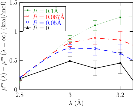
Figure 2: The free energy discrepancy on the basis of Eq. (1b) for TIP3P water at 300K and normal density utilizing different smooth cutoff functions of the form Eq. (23).

With the present generalized theory in hand, we investigated the following idea: Consider a family of cutoff functions for which the softness can be systematically varied. An example is

$$1-b_{m}(r)=\mathrm{e}^{-\left(\lambda/r\right)^{m}}$$ (24)

with a parameter $m>3$. With increasing $m$ this cutoff becomes increasingly sharp. A natural idea then is to choose $m$ to minimize the variance of the conditional distribution $P(\varepsilon|\chi=1)$ appearing in Eq. (1a). The goal is to narrow the distribution so that deviations from the gaussian model for $\mu^{\mathrm{ex}}$ (Eq. (1b)) are less important. We found that the variance decreases with increasing $m$ (increasing sharpness) towards an $m\sim\infty$ limiting value, the hard-cutoff case as a practical matter. Hard-cutoff conditioning is always preferred for such cases. The conclusion is that for systems and calculations such as these, the results are always improved the more that the conditioning eliminates statistical modeling of short-ranged interactions, and hard cutoffs do that best. Those interactions include both associative and repulsive interactions that encompass both chemical and packing contributions. This conclusion is clearly consistent with the results shown in FIG. 2.

IV Conclusions

Quasi-chemical theory with a soft-cutoff can be developed in straightforward analogy with the hard-cutoff theory. This development has important practical consequences in the common cases that the packing contribution dominates the solvation free energy of realistically-modeled molecules because treatment of hard-core interactions usually require special purpose simulation methods. In contrast, treatment of smooth repulsive interactions is typically straightforward on the basis of widely available software. This development also shows how fluids composed of molecules with smooth repulsive interactions can be treated analogously to the molecular-field theory of the hard-sphere fluid.PrattLawrenceR.:Selmft

In the treatment of liquid water, soft-cutoff conditioning doesn’t change the fundamental convergence characteristics of the hard-cutoff approach. Hard cutoffs are found to work better than softer ones in that case.

V Acknowledgment

This work was carried out under the auspices of the National Nuclear Security Administration of the U.S. Department of Energy at Los Alamos National Laboratory under Contract No. DE-AC52-06NA25396.

References

- (1) Pratt, L. R.; LaViolette, R. A.; Gomez, M. A.; Gentile, M. E., J. Phys. Chem. B 2001, 105, 11662–11668.
- (2) Paulaitis, M. E.; Pratt, L. R., Adv. Prot. Chem. 2002, 62, 283–310.
- (3) Beck, T. L.; Paulaitis, M. E.; Pratt, L. R., The potential distribution theorem and models of molecular solutions, Cambridge: Cambridge University Press, 2006.
- (4) Pratt, L. R.; Asthagiri, D., in C. Chipot; A. Pohorille, editors, Free Energy Calculations. Theory and Applications in Chemistry and Biology, Berlin: Springer, 2006 pages 323 – 352.
- (5) Rempe, S. B.; Pratt, L. R.; Hummer, G.; Kress, J. D.; Martin, R. L.; Redondo, A., J. Am. Chem. Soc. 2000, 122, 966–967.
- (6) Asthagiri, D.; Pratt, L. R.; Paulaitis, M. E.; Rempe, S. B., J. Am. Chem. Soc. 2004, 126, 1285 – 1289.
- (7) Shah, J.; Asthagiri, D.; Pratt, L.; Paulaitis, M., J. Chem. Phys. 2007, 127, 144508.
- (8) Asthagiri, D.; Ashbaugh, H.; Piryatinski, A.; Paulaitis, M.; Pratt, L., J. Am. Chem. Soc. 2007, 129, 10133 – 10140.
- (9) Asthagiri, D.; Merchant, S.; Pratt, L. R., J. Chem. Phys. 2008, 128, 244512.
- (10) Pratt, L. R.; Ashbaugh, H. S., Phys. Rev. E 2003, 68, 021505/1 – 021505/6.
- (11) Stratt, R.; Holmgren, S.; Chandler, D., Mol. Phys. 1981, 42, 1233–1143.
- (12) Smith, S. W.; Hall, C. K.; Freeman, B. D., J. Comp. Phys. 1997, 134, 16–30.
- (13) Chempath, S.; Pratt, L. R., J. Phys. Chem. B 2008, in press.
- (14) Bennett, C. H., J. Comp. Phys. 1976, 22, 245 – 68.
- (15) Beck, T. L.; Paulaitis, M. E.; Pratt, L. R., The potential distribution theorem and models of molecular solutions, Cambridge: Cambridge University Press, 2006.
- (16) Web site for obtaining source code given in this paper and other potentially useful modules. [www http://zeolites.cqe.northwestern.edu/Music/music.html].
- (17) Gupta, A.; Chempath, S.; Sanborn, M. J.; Clark, L. A.; Snurr, R. Q., Mol. Simul. 2003, 29, 29–46.
- (18) Mahoney, M. W.; Jorgensen, W. L., J. Chem. Phys. 2000, 112, 8910 – 22.
- (19) Paschek, D., J. Chem. Phys. 2004, 120, 6674.
- (20) Fennell, C. J.; Gezelter, J. D., J. Chem. Phys. 2006, 124, 234104 – 1.