A simple formula for the Casson-Walker invariant

Abstract.

Gauss diagram formulas are extensively used to study Vassiliev link invariants. Now we apply this approach to invariants of 3-manifolds, considering a manifold as a result $M_{L}$ of surgery on a framed link $L$ in $S^{3}$. We study the lowest degree case – the celebrated Casson-Walker invariant $\lambda_{w}$ of rational homology spheres. This paper is dedicated to a detailed treatment of 2-component links; a general case will be considered in a forthcoming paper. We present simple Gauss diagram formulas for $\lambda_{w}(M_{L})$. This enables us to understand/separate the dependence of $\lambda_{w}(M_{L})$ on $L$ (considered as an unframed link) and on the framings. We also obtain skein relations for $\lambda_{w}(M_{L})$ under crossing changes of $L$, and study an asymptotic behavior of $\lambda_{w}(M_{L})$ when framings tend to infinity. Finally, we present results of extensive computer experiment on calculation of $\lambda_{w}(M_{L})$.

1. Introduction

One of the simplest types of formulas for Vassiliev invariants are so-called Gauss diagram formulas. An invariant is calculated by counting (with weights) subdiagrams of a special combinatorial type in a given link diagram. The simplest example is counting with signs crossings of two link components to get their doubled linking number. This approach to finite type invariants was successfully and extensively used for invariants of both classical and virtual links (see e.g.[6, 17]).

As a rule, techniques developed for link invariants were usually later applied for 3-manifold invariants using the surgery description of 3-manifolds. Indeed, configuration spaces integrals (arising from the perturbative Chern-Simons theory) and the Kontsevich integral were all adjusted and applied for 3-manifold invariants. Surprisingly, the simplest of those – the Gauss diagram technique – was not, until now, applied to invariants of 3-manifolds.

We start filling this gap by studying the case of the lowest degree, namely the celebrated Casson invariant $\lambda(M_{L})$ (or rather its generalized versions – the Casson-Walker invariant $\lambda_{w}(M)$ and the Lescop invariant $\lambda_{L}(M)=\frac{|H_{1}(M)|}{2}\lambda_{w}(M)$, see  [21, 10]). Note that $\lambda_{w}(M)$ is one of the fundamental invariants of rational homology spheres. The restriction of $\frac{1}{2}\lambda_{w}(M)$ to the class of integer homology spheres is an integer extension of the Rokhlin invariant  [1, 21]. In the theory of finite type invariants of 3-manifolds (see e.g.  [5]) it is the simplest $\mathbb{Q}$-valued invariant after $|H_{1}(M)|$. However, $\lambda_{w}(M)$ remains in general quite difficult to calculate. While it is easy to do for a manifold $M_{K}$ obtained from $S^{3}$ by integer surgery on a framed knot $K$, the same question for links remains quite complicated, apart from the well-studied simple case of unimodular algebraically split links. In particular, for 2-component links satisfactory formulas only exist for some special cases [9]. Formulas from [10], although explicit, were not much applied or studied, possibly due to a large number of terms of various nature and their complicated or cumbersome definitions. While Lescop’s general formulas for $\lambda_{L}(M)$ seem to imply all other formulas of [9, 7, 8], including also formulas of this paper, we feel that a simple explicit formula remains of a considerable interest.

Our approach is elementary, so allows a simple computation of the invariant directly from any integer-framed link diagram and makes many of its properties transparent. We proceed by the number of components of a given framed link $L$. When $L$ is a knot, $\lambda_{w}(M_{L})$ is closely related to the simplest finite type knot invariant $v_{2}$ – the second coefficient of the Alexander-Conway polynomial. So its properties are easy to study knowing the behavior of $v_{2}$; in particular, the Gauss diagram formula is well-known (see [16, 17]). This paper is dedicated to a similar detailed treatment of the 2-component case. The general $n$-component case will be discussed in a forthcoming paper.

A special case of two component links with zero-framed components was studied in [9]. While the invariant is described there only by means of its behavior under a self-crossing of one of the components, a Gauss diagram formula is in fact implicit there. We show that their results extend to the case of arbitrary integer framings and provide a simple Gauss diagram formula in this general case. The main ingredient of this formula appeared first in [16] and is now known as the generalized Sato-Levine invariant, see [2, 3, 9, 13]. The Gauss diagram formula enables us to calculate the values of $\lambda_{w}(M_{L})$ in a simple and straightforward way starting from any diagram of a 2-component link.

Our additional goal is to understand and separate the dependence of $\lambda_{w}(M_{L})$ on the underlying topological type of the link and on the framings. This is also evident from the formula. In particular, we observe an interesting asymptotics of the Casson-Walker invariant as both (or just one of) the framings are rescaled and taken to infinity. It is interesting that in two special cases the asymptotical behavior of $\lambda_{w}(M_{L})$ turns out to be very different from the general case. The first case appears when the framing of one of the components is zero. This could be expected and reflects the fact that the manifold obtained by surgery on this component is not a homology sphere. Another – somewhat more surprising – special case is when the framings of two components are opposite to each other.

We also deduce a simple skein relation for $\lambda_{w}(M)$ which relates its change under a crossing change between two components to its values on the smoothed link and the sublinks.

This has interesting implications for the theory of finite type (or perturbative) invariants of 3-manifolds. Indeed, this theory is well-studied only for integer homology spheres, and thus was defined only on special classes of surgery links, with a complicated Borromean-type modification [12] playing the role of a crossing change. The behavior of an invariant under a self-crossing of one of the link components $L_{i}$ easily fits into the theory (since it may be obtained by adding a new small 1-framed component going around two strands of $L_{i}$ near the crossing), and thus is well-understood [8]. A crossing change between different components, however, changes the homology of the resulting manifold, so does not fit the theory of finite type invariants of 3-manifolds. Our work implies, however, that the relation between finite type invariants of links and 3-manifolds is closer than one could expect and that the behavior of these invariants under such crossing changes may be understood as well.

We remark that while in this paper we usually restrict our consideration to the case when $M_{L}$ is a rational homology sphere, our formulas are well defined also in case when $M_{L}$ is not such. In this case our formula gives the Lescop’s generalization of the Casson-Walker invariant.

We sum up the goals of this paper in the following

Problem. Given a framed 2-component link $L=\{L_{1},L_{2}\}$ with the integer linking matrix $\mathbb{L}$, we want to

1. Find simple Gauss diagram formulas for $\lambda_{w}(M_{L})$;

2. Understand/separate the dependence of $\lambda_{w}(M_{L})$ on $L$ (considered as an unframed link) and on $\mathbb{L}$.

3. Obtain skein relations for $\lambda_{w}(M_{L})$ under crossing changes of $L$.

4. Study an assymptotic behavior of $\lambda_{w}(M_{L})$ when framings tend to infinity.

We thank Nikolai Saveliev for useful discussions and Vladimir Tarkaev for writing a computer program. The main results of the paper have been obtained during the stay of both authors at MPIM Bonn. We thank the institute for hospitality, creative atmosphere, and support.

2. Arrow diagrams

Let $A$ be an oriented 3-valent graph whose edges are divided into two classes: fat and thin. The union of all vertices and all fat edges of $A$ is called a skeleton of $A$.

Definition 2.1.

$A$ is called an arrow diagram, if the skeleton of $A$ consists of disjoint circles. Thin edges are called arrows.

It follows from the definition that each arrow connects two vertices, which may lie in the same circle or in different circles. By a based arrow diagram we mean an arrow diagram with a marked point in the interior of one of its fat edges. See Fig. 1 for simple examples of based and unbased arrow diagrams.

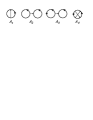
Figure 1. Simple examples of arrow diagrams.

3. Gauss diagrams

Recall that an $n$-component link diagram is a generic immersion of the disjoint union of $n\geq 1$ oriented circles to plane, equipped with the additional information on overpasses and underpasses at double points. Any link diagram can be presented numerically by its Gauss code, which consists of several strings of signed integers. The strings are obtained by numbering double points and traversing the components. Each time when we pass a double point number $k$, we write $k$ if we are on the upper strand and $-k$ if on the lower one. If we prefer to distinguish knots and their mirror images or if we are considering a link with $\geq 2$ components, then an additional string of $\varepsilon_{i}=\pm 1$ called chiral signs is needed. Here $i$ runs over all double points $a_{i}$ of the diagram and signs are determined by the right hand grip rule. See Fig. 2.

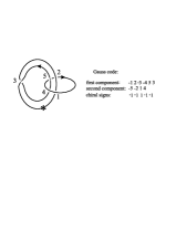
Figure 2. A 2-component link and its Gauss code

A convenient way to visualize a Gauss code is a Gauss diagram consisting of the oriented link components with the preimages of each double point connected with an arrow from the upper point to the lower one. Each arrow $c$ is equipped with the chiral sign of the corresponding double point. The numbering of endpoints of arrows is not necessary anymore, see Fig. 3. We say that a link diagram is based if a non-double point in one of its components is chosen. An equivalent way of saying this consists in considering long links in $R^{3}$, when the base point is placed in infinity. If the link is based, then the corresponding Gauss diagram is based too. Note that forgetting signs converts any Gauss diagram into an arrow diagram, but not any arrow diagram (for example, a fat circle with two thin oriented diameters) can be realized by a Gauss diagram of a link. However, that is possible, if we allow virtual links. This is actually the main idea of the virtualization.

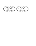
Figure 3. Two presentations of the Gauss diagram for the link diagram in Fig. 2

4. Arrow diagrams as functionals on Gauss diagrams

As described in [16, 6], any arrow diagram $A$ defines an integer-valued function $\left<A,*\right>$ on set of all Gauss diagrams. Let $A$ be an $n$-component arrow diagram and $G$ be an $n$-component Gauss diagram. By a representation of $A$ in $G$ we mean an embedding of $A$ to $G$ which takes the circles and arrows of $A$ to the circles, respectively, arrows of $G$ such that the orientations of all circles and arrows are preserved. If both diagrams are based, then representations must respect base points. For a given representation $\varphi\colon A\to G$ we define its sign by $\varepsilon(\varphi)=\prod\varepsilon(\varphi(a))$, where the product is taken over all arcs $a\in A$.

Definition 4.1.

Let $A$ be an $n$-component arrow diagram. Then for any $n$-component arrow diagram $G$ we set $\left<A,G\right>=\sum\varepsilon(\varphi)$, where the sum is taken over all representations of $A$ in $G$.

Example 4.2.

Let us describe functions for arrow diagrams $A_{1}-A_{4}$ shown in Fig. 1. Evidently, $A_{1}$ determines the writhe of the link, which is defined as the sum of the chiral signs of all double points. Let $G$ be a Gauss diagram of an oriented 2-component link $L=L_{1}\cup L_{2}$. Then $\left<A_{2},G\right>=2n$, where $n={\mbox{lk}}(L_{1},L_{2})$ is the linking number of the components. Indeed, for any arrow of $G$ we have exactly one representation of $A_{2}$ to $G$. Therefore, all double points contribute to $\left<A_{3},G\right>$ (not only points where the one preferred component is over the other). If we insert a base point into $A_{2}$ and a base point into $G$ (thus fixing ordering of the two link component), we get $n$ without doubling. It means that $\left<A_{3},G\right>={\mbox{lk}}(L_{1},L_{2})$. The meaning of $\left<A_{4},G\right>$ is more complicated. If $G$ is a Gauss diagram of a knot $K\subset S^{3}$, then $\left<A_{4},G\right>$ is the second coefficient $v_{2}$ of the Conway polynomial of $K$, which is often called the Casson invariant of $K$. See [17] for a diagrammatic description and properties of $v_{2}$.

Example 4.3.

For arrow diagrams $U_{1},U_{2}$ shown in Fig. 4 and the Gauss diagram $G$ shown in Fig. 3, we have $\left<U_{1},G\right>=0$ and $\left<U_{2},G\right>=1$. The image of the unique representation of $U_{2}$ to $G$ contains arrows 2,3,4.

Figure 4. Two arrow diagrams

Remark 4.4.

Often it is convenient to extend Definition 4.1 by linearity to the free abelian group generated by arrow diagrams. Let $A=\sum_{i=1}^{m}k_{i}A_{i}$ be a linear combination of arrow diagrams. In general, the value $\left<A,G\right>$ depends on the choice of the Gauss diagram $G$ of a given link $L$ as well as on the choice of the base point. However, for some carefully composed linear combinations of arrow diagrams the result does not depend on the above choices. This gives a link invariant $\left<A,G\right>$, which we will denote by $A(L)$. It is easy to show that such an invariant is of finite type. Moreover, any finite type invariant of long knots can be presented in such a form. A similar result for links is unknown. See [6].

5. An arrow diagram invariant of degree three

Consider the following linear combination $U=U_{1}+U_{2}+U_{3}+U_{4}$ of arrow diagrams (see Fig. 5).

Figure 5. Remarkable linear combination of arrow diagrams

Example 5.1.

For the link and Gauss diagrams shown in Fig. 2 and Fig. 3 we have $\left<U,G\right>=1-1=0$, since there are only two representations of summands of $U$ in $G$: one representation of $U_{2}$ (see Example 4.3) and one representation of $U_{4}$ with arrows 2,4,5 in its image.

Example 5.2.

For the link and Gauss diagrams shown in Fig. 6 we have $\left<U,G\right>=-1-1=-2$, since no summands of $U$ have representation in $G$ except the first one which has two representations described by arrow triples (2,5,7) and (4,5,7).

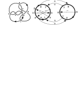
Figure 6. Link $8_{11}^{2}$ in the Alexander-Briggs-Rolfsen table [20].

Let $n$ be an integer and $B$ an unknotted annular band having $n$ negative full twists if $n\geq 0$ and $|n|$ positive full twists if $n<0$, see Fig. 7 for $n=5$. If we equip the components of $\partial B$ by orientations induced by an orientation of $B$, then their linking number is equal to $n$.

Definition 5.3.

The 2-component link $\partial B$ is called the generalized Hopf link and denoted $H(n)$. Denote by $H(n,a,b)$ the generalized Hopf link $H(n)$ with framings $a,b$ of its components.

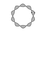
Figure 7. Generalized Hopf link $H(n)$ for $n=5$.

The orientation of components of $\partial B$ induced by an orientation of $B$ is a part of definition of $H(n)$. If we reverse orientation of one of them, we get a new oriented link $\bar{H}(n)$ with the linking number of components $-n$. A diagram of $H(n)$ and $\bar{H}(n)$ for $n=3$ are shown on top and bottom of Fig. 8, respectively.

Example 5.4.

The diagrams of $H(n)$ and $\bar{H}(n)$ mentioned above differ only by orientation of one component. Nevertheless, their Gauss diagrams $G_{n}$ and $\bar{G}_{n}$ look quite different, see Fig. 8 for $n=3$. For $G_{3}$ we have $\left<U,G_{3}\right>=0$, since no summands of $U$ have representation in $G_{3}$. Of course, the same fact holds for any $n$. For the bottom diagram $\bar{G}_{3}$ we get $\left<U,\bar{G}_{3}\right>=-4$. Indeed, in this case there are four representations of $U_{4}$ in $\bar{G}_{3}$. They can be described by four triples of positive arrows (1,2,3),(1,2,5), (1,4,5),(3,4,5) contained in their images. Since $0=\left<U,G_{3}\right>\neq\left<U,\bar{G}_{3}\right>=-4$, we may conclude that the value of $\left<U,G\right>$ depends of orientation of the components. Nevertheless, the following proposition shows that aside this phenomenon $\left<U,G\right>$ is invariant.

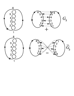
Figure 8. Links $H(3)$ and $\bar{H}(3)$

Proposition 5.5.

$U$ determines an invariant $U(L)=\left<U,G\right>$ for oriented links of two ordered components.

Proof.

We will always assume that the base point is on the first component. It suffices to show that $\left<U,G\right>$ is invariant with respect to

1. Reidemeister moves far from the base point.

2. Replacing the base point within the first component.

In order to verify the invariance under Reidemeister moves, it suffices to show that $\left<U,R\right>=0$, where $R$ runs over all relations of the Polyak algebra $P$ defined in [6].

Invariance of $\left<U,G\right>$ under replacing the base point within the same component follows from the observation that two link diagrams with the common base point in their first components are Reidemeister equivalent if and only if they are equivalent via Reidemeister moves performed far from the common base point. One can give a “folklore” reformulation of that fact by saying that the theory of links is equivalent to the theory of long links (having in mind that the base point is at infinity).  

Once the invariance of $U(L)$ is established, one can identify it with the generalized Sato-Levine invariant $c_{3}(L)-(c_{2}(L_{1})+c_{2}(L_{2}))c_{1}(L)$ (see [2, 3, 9, 13]), where $c_{k}$ is the coefficient at $z^{k}$ of the Conway polynomial. There are several ways to do that. In particular, one may show that $\left<U,G\right>$ does not depend on the ordering of the components of $L$. Then the identification follows from the fact that it is an invariant of degree three for 2-component links and such invariants are classified. So it suffices to check values of $U(L)$ on a few simple links. Another way to identify $U(L)$ is to check that it satisfies a simple skein relation under crossing change of one of the components. Then its values on generalized Hopf links determine the invariant.

We will follow the latter scheme of proof, since it will also be the easiest way to relate the function $\mu(L)$ from Definition 6.1 below and $\lambda_{w}(M_{L})$. Alternatively, instead of checking values of $U(L)$ on generalized Hopf links, one may check that $U(L)$ satisfies an appropriate skein relation under crossing change of two different components (and vanishes on the unlink). This idea will be used in Section 11 to extract a skein formula for the Casson-Walker invariant.

6. The Formula

Let ${L}=L_{1}\cup L_{2}$ be an oriented 2-component framed link. Denote by $a,b$, and $n$ the framings of $L_{1},L_{2}$, and their linking number, respectively. Suppose that the integer linking matrix $\mathbb{L}=\left(\begin{array}[]{cc}a&n\\ n&b\end{array}\right)$ of $L$ has non-zero determinant $D=\mathrm{Det}(\mathbb{L})$. The signature of $\mathbb{L}$ will be denoted by $\sigma$. It is easy to see that $\sigma$ can be found by the following rule:

$$\sigma=\left\{\begin{array}[]{ll}0&\mbox{if $D<0$}\\ 2&\mbox{if $D>0$ and $a+b>0$}\\ -2&\mbox{if $D>0$ and $a+b<0$}\\ \end{array}\right.$$

We point out that if $D>0$, then $a,b$ have the same sign. Therefore, in this case $\sigma$ is determined only by the sign, say, of $a$.

Recall that $v_{2}(K)$ denotes the Casson invariant $\left<A_{4},G_{K}\right>$ of a knot $K\subset S^{3}$ (see Fig. 1 for arrow diagram $A_{4}$). It coincides with the coefficient at $z^{2}$ of the Conway polynomial of $K$. It can also be extracted from the Alexander polynomial $\Delta_{K}(t)$ normalized so that $\Delta_{K}(t^{-1})=\Delta_{K}(t)$ and $\Delta_{K}(1)=1$ as follows: $v_{2}(K)=\frac{1}{2}\Delta_{K}^{\prime\prime}(1)$.

We introduce a function $\mu\colon{\cal L}\to\mathbb{Q}$, where $\cal L$ is the set of all oriented framed 2-component links, as follows. Let $L=L_{1}\cup L_{2}\in{\cal L}$ .

Definition 6.1.

$$\mu(L)=av_{2}(L_{2})+bv_{2}(L_{1})-U(L)+\frac{1}{12}(n^{3}-n)+\frac{1}{24}(a+b)(2n^{2}-ab-2)$$

Example 6.2.

Let us calculate $\mu(L)$, where $L=H(n,a,b)$ is the generalized Hopf link $H(n)$ framed by $a,b$, see Definition  5.3. It is easy to see that $U(H(n))=0$ (see Example 5.4, where we have shown that $U=0$ for $H(3)$). Taking into account that $v_{2}(L_{1})=v_{2}(L_{2})=0$, we get

$$\mu(H(n,a,b))=\frac{1}{12}(n^{3}-n)+\frac{1}{24}(a+b)(2n^{2}-ab-2)$$

Let $M_{L}$ be the manifold obtained by surgery on $L$. Note that our assumption $D\neq 0$ means that the corresponding 3-manifold $M_{L}$ is a rational homology sphere, i.e. the first homology group of $M_{L}$ is finite. Its order $|H_{1}(M_{L})|$ equals to $|D|$.

Let $\lambda_{w}(M_{L})$ be the Casson-Walker invariant of $M_{L}$, see  [21]. We normalize it following Walker, so as to have $\frac{1}{2}\lambda_{w}(P_{120})=1$, where $P_{120}$ is the positively oriented Poincaré homology sphere, obtained from $S^{3}$ by surgery along the trefoil with framing 1.

Theorem 6.3.

(Main) For any oriented framed 2-component link $L=L_{1}\cup L_{2}$ we have

$${\frac{1}{2}D(\lambda_{w}(M_{L})-\frac{1}{4}\sigma)=\mu(L)}$$

.

Example 6.4.

Let us apply the main theorem for calculation of the Casson-Walker invariant $\lambda_{w}$ for the manifold $M_{H(2,3,1)}$, where $H(2,3,1)$ is the Hopf link $H(2)$ framed by $a=3,b=1$ (see Fig. 9).

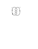
Figure 9. Generalized Hopf link $H(2)$ framed by $3,1$

It follows from Example 6.2 that

$$\frac{1}{2}\lambda_{w}(M_{H(2,3,1)})=\frac{1}{24D}(12+(a+b)(2n^{2}-ab-2)+\frac{1}{8}\sigma.$$

Substituting $D=3\cdot 1-2^{2}=-1$ and $\sigma=0$ we get $\frac{1}{2}\lambda_{w}(M_{H(2,3,1)})=-1$. This is not surprising, since $M_{H(2,3,1)}$ is the negatively oriented Poincaré homology sphere $-P_{120}$. Indeed, one generalized destabilization move (sometimes called blow-down) transforms $H(2,3,1)$ into the left trefoil framed by -1.

The plan of proving the above theorem consists of two steps.

Step 1. We show that the correctness of equality $\frac{1}{2}D(\lambda_{w}(M_{L})-\frac{1}{4}\sigma)=\mu(L)$ is preserved under self-crossing of a link component.

Step 2. We show that the equality is true for the Hopf links $H(n),n\neq 0$ framed by $a,b$. We do that by comparing our formula for $\mu(H(n,a,b))$ (see Example 6.2) with Lescop’s formula for the values of $\lambda_{L}$ for Seifert manifolds (see [10], page 97).

Steps 1,2 imply Theorem 6.3, since any 2-component link can be transformed by self-crossings of its components into a generalized Hopf link.

Let us pause to make few remarks on the role of the function $\mu$.

Remark 6.5.

Theorem 6.3 implies that $\mu(L)$ does not depend on the orientation of the components and is preserved under handle slides. It is not a pure 3-manifold invariant, since some additional information from the surgery link is needed (namely, the sign of $D$ and the signature $\sigma$). However, it may be considered as a convenient renormalization of the Casson invariant for technical purposes, since it is better suited for calculations and has simpler skein properties.

Remark 6.6.

It turns out that $\mu$ may be defined by a similar Gauss diagram formula for $n$-component links with any $n=1,2,3,\dots$. The general case $n\geq 3$ will be discussed in a forthcoming paper. Let us define it for $n=1$. For a framed knot $K$ with framing $a$ we denote

$$\mu(K)=v_{2}(K)-\frac{1}{24}(a^{2}+2),\quad\text{where}\quad v_{2}(K)=\left<A_{4},G_{K}\right>$$

Since values of $\lambda_{w}$ for manifolds obtained by surgery on a framed knot are well-known, it is easy to check that similarly to Theorem 6.3 one indeed has

$${\frac{1}{2}D(\lambda_{w}(M_{K})-\frac{1}{4}\sigma(a))=\mu(K),}$$

where $\sigma(a)$ is the signature of $(1\times 1)$-matrix $(a)$, i.e. the sign of $a$. This may be deduced also from Theorem 6.3, by considering $K$ stabilized by $\pm 1$-component. Now we can rewrite $\mu(L)$ for 2-component links using its values on sublinks:

$$\mu(L)=\mu(L_{1})b+\mu(L_{2})a-U(L)+\frac{1}{12}(n^{3}-n)+\frac{1}{12}(a+b)n^{2}$$

7. Behavior of $\mu$ with respect to self-crossings

Let us carry out Step 1. Suppose that a diagram $G^{-}$ of an oriented framed 2-component link $L^{-}=K^{-}\cup S^{-}$ is obtained from a diagram $G^{+}$ of a framed link $L^{+}=K^{+}\cup S^{+}$ by a single crossing change at a double point $C$ of $K^{+}$ such that the chiral sign of $C$ is 1 in $K^{+}$ and -1 in $K^{-}$. Note that $K^{+}$ can be considered as to consist of two loops (lobes) with endpoints in $C$. Denote by $\ell$ the linking number of the lobes, by $k$ the linking number of one of the lobes with $S^{+}$, and by $n$ the linking number of $K^{+}$ and $S^{+}$. Note that the crossing change preserves the linking matrix $\mathbb{L}^{+}$ of $L^{+}$.

Lemma 7.1.

In the situation above we have

$$\frac{1}{2}D(\lambda_{w}(M_{L^{+}})-\lambda_{w}(M_{L^{-}}))=b\ell-k(n-k)=\mu(L^{+})-\mu(L^{-}),$$

where $D=\mathrm{Det}(\mathbb{L}^{+})$ and $b$ is the framing of $S^{+}$.

Proof.

The first equality is a partial case (for 2-component links) of the crossing change formula, which is the main result of [7].

Let us prove the second one. Since the crossing change preserves the linking matrix, we have $\mu(L^{+})-\mu(L^{-})=bv_{2}(K^{+})-bv_{2}(K^{-})-\left<U,G^{+}\right>+\left<U,G^{-}\right>$. Recall that the equality $v_{2}(K^{+})-v_{2}(K^{-})=\ell$ is one of the main properties of $v_{2}$, see [6]. For the Arf-invariant $v_{2}$ mod 2 it was known long ago, see [12]. It follows that $bv_{2}(K^{+})-bv_{2}(K^{-})=b\ell$.

Let us compute $\left<U,G^{+}\right>-\left<U,G^{-}\right>$. Note that the Gauss diagrams $G^{\pm}$ are almost identical. The only difference between them is that the arrows $a^{+}(C),a^{-}(C)$ corresponding to $C$ have opposite orientations and signs. Let us analyze representations of $U_{k},1\leq k\leq 4,$ in $G^{\pm}$. We call a representation $\varphi\colon U_{k}\to G^{\pm}$ significant, if its image contains $a^{\pm}(C)$. Otherwise $\varphi$ is insignificant. Since $G^{\pm}$ are identical outside $a^{\pm}(C)$, there is a natural bijection between insignificant representations of $U_{k}$ to $G^{+}$ and $G^{-}$ such that the signs of corresponding representations are equal. It follows that insignificant representations do not contribute to the difference $U(L^{+})-U(L^{-})$.

Case 1. Assume that the base point of $L^{+}$ is in $K^{+}$. Denote by $P$ the lobe of $K^{+}$ containing the base point. Let $\bar{P}$ be the other lobe. Consider a significant representation $\varphi\colon U_{k}\to G^{\pm}$. Since $\varphi$ is significant, $a^{+}(C)$ is in its image and thus $k=1$ or $k=2$. Any such representation is completely determined by two arrows of $G^{\pm}$ contained in the image of $\varphi$. One of them connects $P$ to $S^{\pm}$, the other goes from $S^{\pm}$ to $\bar{P}$. It is easy to see that the contribution of $\varphi$ to the difference $U(L^{+})-U(L^{-})$ is equal to the product of the signs of those two arrows. Taking into account Example 4.2 (containing Gauss diagram description of various linking numbers) we may conclude that $U(L^{+})-U(L^{-})=k(n-k)$.

Case 2. Assume that the base point of $L^{+}$ is in $S^{+}$. Since $C$ is in $K^{+}$, there are no significant representations of $U_{1},U_{2},U_{4}$ in $G^{\pm}$. Moreover, any representation $\varphi\colon U_{3}\to G^{\pm}$ is completely determined by two arrows of $G^{\pm}$ contained in the image of $\varphi^{\pm}$. One of them connects $S^{\pm}$ to $P$, the other $S^{\pm}$ to $\bar{P}$. As above, the contribution of $\varphi$ to the difference $U(L^{+})-U(L^{-})$ is equal to the product of the signs of those two arrows. We may conclude that $U(L^{+})-U(L^{-})=k(n-k)$ also in this case.  

Example 7.2.

Let $L^{+}=L_{1}^{+}\cup L_{2}^{+}$ be the link shown in Fig. 10 (all arrows have positive signs). Suppose that $L^{-}=L_{1}^{-}\cup L_{2}^{-}$ is obtained from $L^{+}$ by a crossing change at the double point $C$ having number 1. We assume that the framings of $L_{1}^{+},L_{2}^{+}$ are $a,b$. Note that $n=3$, $k$ is either 1 or 2, and $\ell=1$. Taking into account that $v_{2}(L_{1}^{+})=1$ and $v_{2}(L_{2}^{+})=0$, we get $\mu(L^{+})-\mu(L^{-})=b-2$. Therefore, $\frac{1}{2}D\lambda_{w}(M_{L^{+}})-\frac{1}{2}D\lambda_{w}(M_{L^{-}})=b-2$.

Figure 10. There is only two representations of $U_{k},1\leq k\leq 4$ to $G^{\pm}$, namely a representation $U_{1}\to G^{+}$ having sign 1 and a representation $U_{2}\to G^{-}$ having sign -1. They covers arrows $(1,4,7)$ of $G^{+}$ and $(8,7,\bar{1})$ of $G^{-}$, where $\bar{1}$ denotes the first arrow of $G^{+}$ with reversed orientation. The total contribution of $U$ to $\mu(L^{+})-\mu(L^{-})$ is 2

Corollary 7.3.

Let $L=L_{1}\cup L_{2}$ be an oriented 2-component link in $S^{3}$ and $U$ the linear combination of arrow diagrams shown in Fig. 5. Then the invariant $U(L)=\left<U,G\right>$ does not depend on the ordering of the components of $L$. It coincides with the generalized Sato-Levine invariant $c_{3}(L)-(c_{2}(L_{1})+c_{2}(L_{2}))c_{1}(L)$, where $c_{k}$ is the coefficient at $z^{k}$ of the Conway polynomial.

Proof.

Let us compare values of $U$ for two links which differ only by ordering. By Lemma 7.1 the behavior of $U$ under self-crossings does not depend on the ordering. Thus it suffices to compare values of $U$ on Hopf links $H(n)$ with two different orderings; but Example 5.4 shows that it is $0$ in both cases. The last statement follows from the fact that the generalized Sato-Levine invariant satisfies the same skein relations and also vanishes on $H(n)$.  

8. Model manifolds $Q(n,a,b)$

This section is dedicated to the study of the 3-manifold obtained by surgery on $H(n,a,b)$. To that end, let us introduce another framed link $S(A,B,C)$ shown in Fig. 11. It consists of four unknotted circles framed by $A=a+n,B=b+n,C=-n$, and 0 such that each of the first three circles links the forth circle framed be 0 exactly ones.

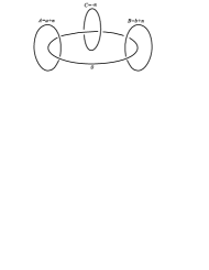
Figure 11. Framed link presenting a Seifert manifold

Lemma 8.1.

Manifolds obtained by Dehn surgery of $S^{3}$ along $H(n,a,b)$ and $S(A,B,C)$ are related by a homeomorphism which preserves orientations induced from the orientation of $S^{3}$.

Proof.

Adding the C-framed component to the components framed by $A,B$ and then removing the 0-framed component together with the $C$-framed one, one can easily show that $S(A,B,C)$ is Kirby equivalent to $H(n,a,b)$.  

Let us denote by $Q=Q(n,a,b)$ the manifold obtained from $S^{3}$ by Dehn surgery along $H(n,a,b)$ or $S(A,B,C)$. Performing surgery of $S^{3}$ along the 0-framed component of $S(A,B,C)$, we get $S^{2}\times S^{1}$ such that the other three components are the fibers of the natural fibration $S^{2}\times S^{1}\to S^{2}$. It follows that $Q$ is a Seifert manifold fibered over $S^{2}$ with three exceptional fibers of types $(A,1),(B,1),(C,1)$ Here we neglect the usual convention that the first parameters of exceptional fibers must be positive. Our goal is to calculate $\mu(Q)$.

Remark 8.2.

As we have seen above, manifolds of the type $M_{H(n,a,b)}$ have a very simple structure: they are Seifert manifolds fibered over $S^{2}$ with three exceptional fibers of type $(p,\pm 1)$. The values of $\mu(M_{H(n,a,b)})$ can certainly be obtained using the main Lescop formula ([10], page 12,13), but we prefer to take into account the specific structure of $M_{H(n,a,b)}$ and use simpler Lescop’s formula ([10], page 97).

Note that the Euler number of $Q$ is $\frac{1}{A}+\frac{1}{B}+\frac{1}{C}$ and the normalized parameters of the exceptional fibers are $(|X|,s(X)$mod$|X|)$, where $X=A,B,C$ and $s(X)$ is the sign of $X$. It turns out that the signature $\sigma$ of $\mathbb{L}$ may be expressed via the signs of $A,B,C$:

Lemma 8.3.

For any numbers $A,B,C$ such that $D=AB+AC+BC\neq 0$, $K=ABC\neq 0$, and $e=D/K>0$ we have $\sigma=s(A)+s(B)+s(C)-1$, where $s(X)$ denotes the sign of $X$ and $\sigma$ is the signature of the matrix $\mathbb{L}=\left(\begin{array}[]{cc}a&n\\ n&b\end{array}\right)$ for $a=A+C,b=B+C,n=-C$.

Proof.

One can extract from Lemma 8.1 that the matrices $\mathbb{L}=\left(\begin{array}[]{cc}a&n\\ n&b\end{array}\right)$ and $\left(\begin{array}[]{cccc}A&0&0&1\\ 0&B&0&1\\ 0&0&C&1\\ 1&1&1&0\end{array}\right)$ have the same signature. It follows that permutations of $A,B,C$ do not affect the correctness of Lemma 8.3. So we may assume that $A\geq B\geq C$.

Suppose that $K>0$. Then $D>0$ and either $A\geq B\geq C>0$ and $\sigma=2s(a)=2s(b)=2$ or $A>0,B<0,C<0$ and $\sigma=2s(a)=2s(b)=-2$. In both cases we get the conclusion of the lemma.

Now suppose that $K<0$. Since $D<0$, we have $\sigma=0$ and exactly one negative number among $A,B,C$. Therefore, $s(A)+s(B)+s(C)=1+\sigma$.  

9. Casson-Walker invariant for model manifolds

Let $M$ be a rational homology sphere. Recall that the Lescop invariant $\lambda_{L}(M)$ is related to the Casson-Walker invariant $\lambda_{w}(M)$ by

$$\lambda_{L}(M)=\frac{1}{2}|H_{1}(M)|\lambda_{w}(M),$$

see [10, 19]. If $M$ is presented by an oriented framed link $L$ with linking matrix $\mathbb{L}$, then we can rewrite that formula as follows:

$$s(D)\lambda_{L}(M)=\frac{1}{2}D\lambda_{w}(M),$$

where $D$ is the determinant of $\mathbb{L}$ and $s(D)$ is the sign of $D$. We will use Lescop formula ([10], page 97) for the Seifert manifold $M=(S^{2};(a_{1},b_{1}),\dots,(a_{m},b_{m})(1,b))$ (in the original notation $M=(Oo0|b;(a_{k},b_{k})_{k=1,\dots,m})$):

$$\lambda_{L}(M)=\left(\frac{sign(e)}{24}\left(2-m+\sum_{k=1}^{m}\frac{1}{a^{2}_{k}}\right)+\frac{e|e|}{24}-\frac{e}{8}-\frac{|e|}{2}\sum_{k=1}^{m}s(b_{k},a_{k})\right)|\prod_{k=1}^{m}a_{k}|,$$

where $0<b_{k}<a_{k}$, $e=b+\sum_{k=1}^{m}b_{k}/a_{k}$ is the Euler number of $M$, and $s(b_{k},a_{k})$ are the Dedekind sums.

Let us recall the definition and properties of $s(b,a)$. If $a,b$ are coprime integers, then $s(b,a)$ is defined by

$$s(b,a)=\sum_{k=1}^{|a|}\left(\left(\frac{k}{a}\right)\right)\left(\left(\frac{kb}{a}\right)\right),$$

where

$$\left(\left(x\right)\right)=\left\{\begin{array}[]{ll}x-[x]-\frac{1}{2}&\mbox{if $x\not\in\mathbb{Z}$}\\ 0&\mbox{if $x\in\mathbb{Z}$}\\ \end{array}\right.$$

is the sawtooth function, see Fig. 12.

Figure 12. The sawtooth function

It follows from the definition that $s(b,a)$ possesses the property $s(b,a)=s(-b,-a)=-s(-b,a)=-s(b,-a)=s(b\pm a,a)$. In particular, $s(b,a)$ only depends on $b$ mod $a$ and $a$.

Proposition 9.1.

Let $Q=Q(n,a,b)$ be obtained by surgery of $S^{3}$ along the framed generalized Hopf link $H(n,a,b)$. Then $\frac{1}{2}D(\lambda_{w}(M)-\frac{1}{4}\sigma)=\mu(H(n,a,b))$, where $\mu(H(n,a,b))$ is given by Example 6.2.

Proof.

Recall from Section 8 that $Q$ is a Seifert manifold fibered over $S^{2}$ with three exceptional fibers of types $(A,1),(B,1),(C,1)$, where $A=a+n,B=b+n,C=-n$. The Euler number of $Q$ is $e=\frac{1}{A}+\frac{1}{B}+\frac{1}{C}$ and the normalized parameters of the exceptional fibers are $(|X|,s(X)\textrm{ mod }|X|)$, where $X=A,B,C$ and $s(X)$ is the sign of $X$.

Note that reversing signs of $n,a,b$ (and hence signs of $A,B,C$ and $e$) does not affect the correctness of the conclusion of the lemma. So we may restrict ourselves to the case $e>0$.

The proof is a cumbersome but straightforward comparison of two expressions. Let us introduce the following notations.

1. $K=ABC$. Then $e=\frac{D}{K}$. Since $e>0$, $K$ and $D$ have the same sign. We denote it by $s(D)$.

2. $P=A^{2}B^{2}+A^{2}C^{2}+B^{2}C^{2}$. Then $\frac{1}{A^{2}}+\frac{1}{B^{2}}+\frac{1}{C^{2}}=\frac{P}{K^{2}}$.

3. $S=AC(B-s(B))(B-2s(B))+AB(C-s(C))(C-2s(C))+BC(A-s(A))(A-2s(A))$. In order to explain the meaning of $S$, we recall that the Dedekind sums $s(1,\ell)$ can be calculated by the rule

   $$s(1,\ell)=\frac{1}{12\ell}(\ell-s(\ell))(\ell-2s(\ell)).$$

   It follows that $s(1,A)+s(1,B)+s(1,C)=\frac{S}{12K}$.

4. $\Sigma=A+B+C$.

Using this notation and applying the above Lescop formula, we get

$$24\lambda_{L}(Q)=\varepsilon(-K+\frac{1}{K}(P+D^{2}-DS)-3D)$$

Simple calculation shows that $P-D^{2}=-2K\Sigma$ and $2D-S=K(3(s(A)+s(B)+s(C))-\Sigma)$. It follows that

$$24\lambda_{L}(Q)=\varepsilon(-K-2\Sigma-D\Sigma+3D(s(A)+s(B)+s(C)-1))$$

and, since $\lambda_{L}(Q)=\frac{\varepsilon D}{2}\lambda_{w}(Q)$,

$$12D\lambda_{w}(Q)=-K-2\Sigma-D\Sigma+3D(s(A)+s(B)+s(C)-1).$$

Let us now substitute $a=A+C,b=B+C,n=-C$ to the expression for $\mu(H(n,a,b))$ (see Example 6.2). We get

$$24\mu(H(n,a,b))=-C^{3}+\Sigma C^{2}-\Sigma D-2\Sigma-CD$$

Let us show that $12D\lambda_{w}(Q)-3D\sigma-24\mu(H(n,a,b))=0$. Performing the substraction, we get

$$12D\lambda_{w}(Q)-3D\sigma-24\mu(H(n,a,b))=\\ -K+3D(s(A)+s(B)+s(C)-1-\sigma)+C^{3}-\Sigma C^{2}+CD$$

or, taking into account that $-K+C^{3}-\Sigma C^{2}+CD=0$,

$$12D\lambda_{w}(Q)-3D\sigma-24\mu(H(n,a,b))=3D(s(A)+s(B)+s(C)-1-\sigma).$$

It remains to note that $s(A)+s(B)+s(C)-1-\sigma=0$ by Lemma 8.3.  

Proof of Main Theorem (which states that $\frac{1}{2}D(\lambda_{w}(M_{L})-\frac{\sigma}{4})=\mu(L)$, see Theorem 6.3). We have realized the plan of the proof indicated in page 6.4. Using Lemma 7.1, we reduce the proof to the partial case of manifolds presented by generalized framed Hopf links. Then we use Proposition 9.1 for proving the theorem in this partial case. $\blacksquare$

10. Asymptotic behavior of the Casson-Walker invariant

Let $L=L_{1}\cup L_{2}$ be an oriented framed 2-component link. Then $\lambda_{w}(M_{L})$ depends on the underlying link and on the framing. Theorem 6.3 allows us to understand the contribution of those two ingredients. We use that for describing the asymptotic behavior of $\lambda_{w}$ as the parameters of the framing tend to $\infty$. For simplicity we restrict ourselves to the simplest case when they have the form $a=a_{0}t,b=b_{0}t$ and $t\to\infty$.

Theorem 10.1.

Let a 3-manifold $M_{t}$ be obtained by surgery of $S^{3}$ along a framed link $L=L_{1}\cup L_{2}$ having linking matrix $\mathbb{L}(t)=\left(\begin{array}[]{cc}a_{0}t&n\\ n&b_{0}t\end{array}\right)$. Then the following holds.

Case 1. Suppose that $a_{0}+b_{0}\neq 0$ and $a_{0}b_{0}\neq 0$. Then

$$\lambda_{w}(M_{t})=-\frac{1}{12}(a_{0}+b_{0})t+\frac{1}{4}\sigma+r(t),$$

where $\sigma$ is the signature of $\mathbb{L}(1)$ and $r(t)\to 0$ as $t\to\infty$.

Case 2. Suppose that $a_{0}+b_{0}=0$ and $a_{0}b_{0}\neq 0$. Then

$$\lambda_{w}(M_{t})=2\frac{v_{2}(L_{1})-v_{2}(L_{2})}{a_{0}}t^{-1}+r(t),$$

where $r(t)t\to 0$ as $t\to\pm\infty$.

Case 3. Suppose that $a_{0}b_{0}=0$. In order to be definite, we assume that $b_{0}=0$. Then

$$\lambda_{w}(M_{t})=-\frac{a_{0}}{6n^{2}}(n^{2}-1+12v_{2}(L_{2}))t-\frac{1}{6n^{2}}(n^{3}-n-12U(L))$$

Proof.

Follows easily from Theorem 6.3 and Definition 6.1: we write down an explicit expression for $\lambda_{w}(M_{t})$ and investigate its asymptotic behavior.  

Let us illustrate the behavior of $\lambda_{w}(M_{t})$ graphically for $a_{0}+b_{0}\neq 0$, $a_{0}b_{0}\neq 0$, and $t\to\infty$. The right-hand sides of the expression for $\lambda_{w}(M_{t})$ (see the above proof) and its approximation $-\frac{1}{12}(a_{0}+b_{0})t+\frac{1}{4}\sigma(t)$ make sense for all (not necessarily integer) values of $t$. We show the graphs of these functions for the generalized framed Hopf link $H(n,a_{0},b_{0})$, where $n=2,a_{0}=3,b_{0}=2$ (Fig. 13) and $n=5,a_{0}=-3,b_{0}=2$ (Fig. 14). Both graphs in Fig. 13 have singularities at $t=\frac{n^{2}}{\sqrt{a_{0}b_{0}}}\approx 0.8$ (because of the jump of $\sigma(t)$).

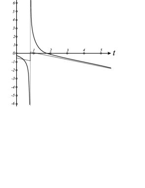
Figure 13. The behavior of $\lambda_{w}(M_{t})$ and its approximation (dotted graph) for $H(2,3,2)$

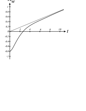
Figure 14. The behavior of $\lambda_{w}(M_{t})$ and its approximation for $H(5,-3,2)$

The following theorem shows the power series presentation of $\lambda_{w}(M_{t})$.

Theorem 10.2.

Let a 3-manifold $M(t)$ be obtained by surgery of $S^{3}$ along a framed link $L=L(t)$ with linking matrix $\mathbb{L}(t)=\left(\begin{array}[]{cc}a_{0}t&n\\ n&b_{0}t\end{array}\right)$. Suppose that $a_{0}b_{0}\neq 0$. Then for $|t|>\frac{|n|}{\sqrt{|a_{0}b_{0}|}}$ we have

$$\lambda_{w}(M_{t})=\frac{1}{2}s(a_{0}b_{0})-\frac{1}{12}(a_{0}+b_{0})t+\\ +\frac{1}{12}\sum_{k=0}^{\infty}\left((C_{1}-C_{3}(a_{0}+b_{0}))C_{3}^{k}t^{-(2k+1)}+C_{2}C_{3}^{k}t^{-(2k+2)}\right),$$

where $s(a_{0}b_{0}$ is the sign of $a_{0}b_{0}$, $C_{1}=\frac{(2n^{2}-2)(a_{0}+b_{0})+24av_{2}(L_{2})+24bv_{2}(L_{1})}{a_{0}b_{0}},$ $C_{2}=\frac{-24U(L)+2n^{3}-2n}{a_{0}b_{0}}$, and $C_{3}=\frac{n^{2}}{a_{0}b_{0}}$.

Proof.

Follows form Theorem 6.3 and Definition 6.1. The infinite series in the expression for $\lambda_{w}(M_{t})$ arises after replacing $D^{-1}=(a_{0}b_{o}t^{2}-n^{2})^{-1}$ by $\frac{t^{-2}}{a_{0}b_{0}}\sum_{k=0}^{\infty}(\frac{n^{2}}{a_{0}b_{0}}t^{-2})^{k}$.  

11. A skein-type relations for $U$ and $\lambda_{w}$

A usual skein relation involves diagrams of three oriented links $L^{+},L^{-},L^{0}$. The diagrams are identical outside a small neighborhood of one positive crossing $C$ of the diagram for $L^{+}$. The diagram of the second link $L^{-}$ is obtained from the diagram of $L^{+}$ by a crossing change at $C$ while the diagram of the oriented knot $L^{0}$ has no crossings at $C$.

We will consider the case when $L^{+}=L^{+}_{1}\cup L^{+}_{2}$, $L^{-}=L^{-}_{1}\cup L^{-}_{2}$ are oriented 2-component links and $C$ is the crossing point of $L^{+}_{1}$ and $L^{+}_{2}$. Then $L^{0}$ is a knot obtained by coherent fusion of $L^{+}_{1}$ and $L_{2}^{+}$, see Fig. 15. We shall refer to any triple $(L^{+},L^{-},L^{0})$ of the above type as an admissible skein triple.

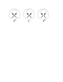
Figure 15. Three links participating in the skein-type relation

Lemma 11.1.

For any admissible skein triple $(L^{+},L^{-},L^{0})$ we have $U(L^{+})-U(L^{-})=v_{2}(L^{0})-v_{2}(L_{1})-v_{2}(L_{2})$.

Proof.

The statement may be deduced from the identification of $U$ with the generalized Sato-Levine invariant, see Corollary 7.3. For completeness we provide a simple direct proof using only the definition of $U$. Denote by $G^{+},G^{-},G^{0}$ Gauss diagrams corresponding to the diagrams of $L^{+},L^{-},L^{0}$. The Gauss diagrams are almost identical. The only difference between $G^{+}$ and $G^{-}$ is that the arrows $a^{+}(C),a^{-}(C)$ corresponding to $C$ have opposite orientations and signs. Knot diagram $G^{0}$ is obtained by coherent fusion of the circles of $G^{+}$ along $a^{+}(C)$. Chose a base point in the first circle of $G^{+}$ just before the initial point of $a^{+}(C)$. We may assume that there are no endpoints of other arrows on small arcs containing the endpoints of $a^{+}(C),a^{-}(C)$, and on arcs of $L^{0}$ obtained by their fusion. See Fig. 16, where those free-of-endpoints arcs are shown dotted and the complementary arcs are numbered by 1,2. For reader’s convenience we have also placed arrows diagrams for $U$ and $v_{2}$.

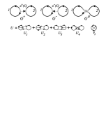
Figure 16. Skein triple of Gauss diagrams

Let us analyze representations of $U_{k},1\leq k\leq 4,$ in $G^{\pm}$. As in the proof of Lemma 7.1, we call a representation $\varphi\colon U_{k}\to G^{\pm}$ significant, if its image contains $a^{\pm}(C)$. Insignificant representations do not contribute to the difference $U(L^{+})-U(L^{-})$.

Let $\varphi$ be a significant representation of $U_{k},1\leq k\leq 4,$ in $G^{\pm}$ and let $a_{k}\subset U_{k}$ be the first arrow we meet travelling from the base point along the first circle of $U_{k}$. Then the careful choice of the base point for $G^{\pm}$ tells us that $\varphi$ takes $a_{k}$ to $a^{\pm}(C)$. It follows that there is no significant representation of $U_{1}$ in $G^{\pm}$ (since the endpoints of $a_{1}$ lie in the same circle of $U_{1}$ while the endpoints of $a^{\pm}(C)$ lie in different circles of $G^{\pm})$.

By similar reason there are no significant representations of $U_{k},2\leq k\leq 4$ in $G^{-}$. Indeed, $a_{k}$ is directed from the first circle of $U_{k}$ to the second one while $a^{-}(C)$ is directed from the second circle of $G^{-}$ to the first one.

Suppose that $\varphi$ is a significant representation of $U_{k},2\leq k\leq 4$ in $G^{+}$. Let us coherently fuse the circles of $U_{k}$ along $a_{k}$. It is easy to see that we get an arrow diagram $A_{4}$ (shown in Fig. 1 and Fig. 16) for calculation of $v_{2}$, together with the corresponding representation $\varphi^{\prime}\colon A_{4}\to G^{0}$. The values of $\varphi$ and $\varphi^{\prime}$ are equal. Vice versa, any representation $A_{4}\to G^{0}$ such that arrows do not all land on the image (under fusion) of the same circle of $G^{+}$, determines a representation $U_{k}\to G^{+}$ having the same value. The only representations $A_{4}\to G^{0}$ which have no corresponding representation $U_{k}\to G^{+}$ are actually representations of $A_{4}$ in the Gauss diagram either of the first or the second circle of $G^{+}$. It follows that $U(L^{+})-U(L^{-})=v_{2}(L^{0})-v_{2}(L_{1})-v_{2}(L_{2})$.  

As a result we get the following behavior of $\lambda_{w}$ under a crossing change involving two components:

Theorem 11.2.

For any admissible skein triple $(L^{+},L^{-},L^{0})$ we have

$$\mu(L^{+})-\mu(L^{-})=v_{2}(L_{1})+v_{2}(L_{2})-v_{2}(L^{0})+\frac{1}{4}(n^{2}-n)+\frac{1}{12}(a+b)(2n-1)$$

thus

$$\frac{D^{+}}{2}\lambda_{w}(L^{+})-\frac{D^{-}}{2}\lambda_{w}(L^{-})=\frac{D^{+}}{8}\sigma^{+}-\frac{D^{-}}{8}\sigma^{-}+\\ +v_{2}(L_{1})+v_{2}(L_{2})-v_{2}(L^{0})+\frac{1}{4}(n^{2}-n)+\frac{1}{12}(a+b)(2n-1)$$

Proof.

Directly follows from Lemma 11.1 and Theorem 6.3.  

12. An Alternative Formula

Consider the following linear combination $U^{\prime}=U_{1}+U_{2}+\frac{1}{2}(U_{3}+U_{3}^{\prime})+\frac{1}{2}(U_{4}-U_{4}^{\prime})$ of arrow diagrams, see Fig. 17.

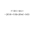
Figure 17. Another remarkable linear combination of arrow diagrams

Lemma 12.1.

Let $L=L_{1}\cup L_{2}$ be an oriented 2-component link. Denote by $L^{\prime}$ the link $L_{1}\cup L^{\prime}_{2}$ obtained from $L$ by reversing the orientation of the second component. Let $G$ and $G^{\prime}$ be their based Gauss diagrams (assuming that the base points are in the first components). Then $\left<U_{1},G\right>=\left<U_{1},G^{\prime}\right>$, $\left<U_{2},G\right>=\left<U_{2},G^{\prime}\right>$, $\left<U_{3},G\right>=\left<U^{\prime}_{3},G^{\prime}\right>$, $\left<U_{4},G\right>=-\left<U^{\prime}_{4},G^{\prime}\right>$, and $\left<U^{\prime},G\right>=\frac{1}{2}\left(\left<U,G\right>+\left<U,G^{\prime}\right>\right)$.

Proof.

Note that $G$ and $G^{\prime}$ actually coincide. The only difference is that their second circles have opposite orientations and that arrows joining different circles have opposite signs. First two equalities of the conclusion of the lemma are evident, since any representation of $U_{i},i=1,2,$ to $G$ determines a representation of $U_{i}$ to $G^{\prime}$, and vice-versa. The images of those representations contains the same arrows. Since exactly two of these arrows join differen components, the values of the representations are equal. Similarly, any representation of $U_{j},j=3,4$ determines a representation of $U^{\prime}_{j}$ to $G^{\prime}$, and vice-versa. The values of those representations are the same for $j=3$ and have opposite signs for $j=4$. This is because the number of arrows in the images of representations is 2 for $j=3$ and 3 for $j=4$. Taking the sums, we get $\left<U^{\prime},G\right>=\frac{1}{2}\left(\left<U,G\right>+\left<U,G^{\prime}\right>\right)$.  

The following proposition and theorem are similar to Proposition 5.5 and Theorem 6.3.

Proposition 12.2.

$U^{\prime}$ determines an invariant $U^{\prime}(L)=\left<U^{\prime},G\right>$ for non-oriented links of two numbered components.

Proof.

It follows from Lemma 12.1 that $\left<U^{\prime},G\right>=\frac{1}{2}\left(\left<U,G\right>+\left<U,G^{\prime}\right>\right)$. Therefore, $U^{\prime}(L)=\left<U^{\prime},G\right>$ is an invariant of oriented links by Proposition 5.5. On the other hand, $\left<U^{\prime},G\right>$ is invariant under reversing orientation of one of its components, since the above expression for it is symmetric.  

Theorem 12.3.

For any non-oriented framed 2-component link $L=L_{1}\cup L_{2}$ we have $\displaystyle{\frac{1}{2}D(\lambda_{w}(M_{L})-\frac{1}{4}\sigma)=\mu^{\prime}(L)}$, where

$$\mu^{\prime}(L)=av_{2}(L_{2})+bv_{2}(L_{1})-U^{\prime}(L)+\frac{1}{24}(a+b)(2n^{2}-ab-2)$$

Proof.

Let us orient $L$ and denote by $L^{\prime}$ the oriented framed link obtained from $L$ by reversing orientation of $L_{2}$. Note that the linking number $n$ of the components of $L$ and the linking number $n^{\prime}$ of the components of $L^{\prime}$ have the same modules and different signs, that is, $n^{\prime}=-n$. All other variables in the expressions for $\mu(L)$ and $\mu(L^{\prime})$ (see Definition 6.1) except of $U(L),U(L^{\prime})$ are the same. In other words, $a,b,D,\sigma$ and both $v_{2}$ for $L$ coincide with the corresponding variables for $L^{\prime}$. It follows from Lemma 12.1 that $\mu^{\prime}(L)=\frac{1}{2}(\mu(L)+\mu(L^{\prime})$. Since $\mu(L)=\frac{1}{2}D(\lambda_{w}(M_{L})-\frac{1}{4}\sigma)=\frac{1}{2}D(\lambda_{w}(M_{L^{\prime}})-\frac{1}{4}\sigma)=\mu(L^{\prime})$ by Theorem 6.3, we get the conclusion.  

13. Results of computer experiments

The formula for $\lambda_{w}(M)$ from Theorem 6.3 is very convenient for calculation. If a diagram of a link framed by integers of reasonable size has about a dozen crossing points, then the manual calculation takes a few minutes. A simple computer program written by V. Tarkaev accepts Gauss codes and takes only seconds for calculating $\lambda_{w}$ for framed links with thousands crossings. We present here a few results of calculation $\lambda_{w}$ for all rational homology 3-spheres which can be presented by diagrams of 2-component (but not of 1-component) links with $\leq 9$ crossings and black-board framings. We thank S. Lins, who kindly prepared for us a list of Gauss codes of those links.

• Number of different manifolds: 194

• Number of different values of $|\lambda_{w}|$ for these manifolds: 66

• Numbers of different manifolds having given values of $|\lambda_{w}|$ are presented in Table 1.

$\mathbf{|\lambda_{w}|}$	$\mathbf{\#M^{3}}$		$\mathbf{|\lambda_{w}|}$	$\mathbf{\#M^{3}}$		$\mathbf{|\lambda_{w}|}$	$\mathbf{\#M^{3}}$		$\mathbf{|\lambda_{w}|}$	$\mathbf{\#M^{3}}$
$0$	$19$		$9/64$	$1$		$11/36$	$4$		$25/44$	$1$
$1/64$	$1$		$4/27$	$2$		$5/16$	$7$		$16/27$	$1$
$1/36$	$4$		$5/32$	$1$		$9/28$	$2$		$3/5$	$1$
$1/32$	$1$		$11/64$	$1$		$11/32$	$2$		$23/36$	$6$
$1/28$	$2$		$5/28$	$1$		$9/26$	$1$		$11/16$	$3$
$1/26$	$1$		$3/16$	$10$		$13/36$	$2$		$25/36$	$3$
$3/64$	$1$		$5/26$	$1$		$10/27$	$2$		$23/32$	$1$
$1/16$	$8$		$7/36$	$1$		$3/8$	$5$		$29/36$	$1$
$3/44$	$1$		$1/5$	$4$		$25/64$	$1$		$15/16$	$3$
$2/27$	$2$		$13/64$	$1$		$2/5$	$1$		$1$	$7$
$5/64$	$1$		$9/44$	$1$		$13/32$	$1$		$19/16$	$1$
$3/32$	$2$		$2/9$	$5$		$19/44$	$1$		$3/2$	$1$
$1/10$	$2$		$15/64$	$1$		$7/16$	$5$		$2$	$16$
$5/44$	$2$		$1/4$	$5$		$4/9$	$2$		$3$	$2$
$3/26$	$1$		$13/44$	$2$		$13/28$	$1$		$4$	$6$
$1/8$	$4$		$8/27$	$2$		$17/36$	$4$		$-$	$-$
$5/36$	$2$		$3/10$	$1$		$1/2$	$6$		$-$	$-$

Table 1. How many manifolds have a given value of $|\lambda_{w}|$

We see from the table that for the set of 194 manifolds under consideration the most popular values of $|\lambda_{w}|$ are $0$ (19 manifolds), $2$ (16 manifolds), $3/16$ (10 manifolds), $1/16$ (8 manifolds), $5/16$ and $1$ (7 manifolds each). Exactly 30 values of $|\lambda_{w}|$ are taken by only one manifold each. In other words, those manifolds are determined by $|\lambda_{w}|$. In average, each value is taken by only 3 different manifolds from the list. This shows that the Casson-Walker invariant is unexpectedly informative. For example, the number of different first homology groups of the manifolds under consideration is 17, so the average number of manifolds having a given group is about 11.4.

References

- [1] Akbulut, S., McCarthy, J. D. Casson’s invariant for oriented homology -spheres. An exposition. // Mathematical Notes, 36. Princeton University Press, Princeton, NJ, (1990). xviii+182 pp.
- [2] Akhmetiev, P. M., Malešič, J., Repovš, D. A formula for the generalized Sato–Levine invariant. // Mat. Sbornik 192:1 (2001), 3–12; English transl. Sb. Math. (2001) 1–10.
- [3] Akhmetiev, P. M., Repovš, D. A generalization of the Sato–Levine invariant. // Trudy Mat. Inst. im. Steklova 221 (1998), 69–80; English transl. Proc. Steklov Inst. Math. 221 (1998), 60–70.
- [4] Hoste, J. A formula for Casson’s invariant. // Trans. A.M.S. 297 (1986), 547–562.
- [5] Garoufalidis, S., Goussarov, M., Polyak, M. Calculus of clovers and finite type invariants of 3-manifolds. // Geometry and Topology 5 (2001), 75–108.
- [6] Goussarov, M., Polyak M., Viro O. Finite-type invariants of classical and virtual knots. // Topology 39 (2000), no. 5, 1045–1068.
- [7] Johannes, J. A Type 2 polynomial invariant of links derived from the Casson-Walker invariant. // J. Knot Theory Ramifications 8 (1999), 491–504.
- [8] Johannes, J. The Casson-Walker-Lescop invariant and link invariants // J. Knot Theory Ramifications 14:4 (2005), 425–433.
- [9] Kirk, R., Livingston, C. Vassiliev invariants of two component links and the Casson-Walker invariant // Topology 36 (1997), 1333–1353.
- [10] Lescop, C. Global surgery formula for Casson-Walker invariant // Annals of Mathematics Studies 140, Princenton University Press, Princenton, (1996).
- [11] Livingston, C. Enhanced linking numbers // Amer. Math. Monthly 110 (2003) 361–385.
- [12] Matveev, S. Generalized surgery of 3-manifolds and representations of homology spheres. // Mat. Zametki 42 (1987), 268-278 (English translation in: Math. Notices Acad. Sci. USSR 42:2 (1987), 651–656).
- [13] Melikhov, S. Colored finite type invariants and a multi-variable analogue of the Conway polynomial // preprint math.GT/0312007 (2003).
- [14] Nakanishi, Y., Ohyama, Y. Delta link homotopy for two component links, III // J. Math. Soc. Japan 55:3, (2003), 641–654
- [15] Polyak, M. On the algebra of arrow diagrams. // Lett. Math. Phys. 51:4, (2000), 275–291.
- [16] Polyak, M., Viro, O. On the Casson knot invariant. // Knots in Hellas ’98, Vol. 3 (Delphi). J. Knot Theory Ramifications 10 (2001), no. 5, 711–738.
- [17] Polyak, M., Viro, O. Gauss diagram formulas for Vassiliev invariants. // Internat. Math. Res. Notices (1994), no. 11, 445ff., approx. 8 pp. (electronic).
- [18] Saveliev, N. Lectures on the Topology of 3-Manifolds. An introduction to the Casson invariant // Walter de Gruyter, (1999).
- [19] Saveliev, N. Invariants for Homology 3-spheres // Springer (2003).
- [20] Rolfsen, D. Knots and Links // Mathematics Lecture Series 7, Publish of Perish, Houston (1976).
- [21] Walker, K. An extension of Casson’s invariant, // Annals of Mathematics Studies 126, Princeton University Press, Princeton (1992).