Transverse momentum of partons:
from low to high pT

Abstract:

Transverse-momentum spectra in hard processes are typically described either in terms of intrinsic transverse momentum of partons, or in terms of perturbative radiation. The relation between these descriptions is discussed for the example of semi-inclusive deep inelastic scattering, with special focus on the angular distribution of the observed hadron. This involves nontrivial theoretical issues, such as the proper definition of transverse-momentum dependent parton distributions, and has practical consequences for the description of $p_{T}$ spectra in phenomenology.

1 Motivation

This talk is concerned with the transverse-momentum dependence of particles produced in scattering processes involving a hard momentum scale. Specifically, I will discuss semi-inclusive deep inelastic scattering, $ep\to e+h+X$, where the momentum of the hadron $h$ is measured. Using crossing symmetry, the results can be carried over to Drell-Yan or $W$ or $Z$ production in $pp$ and $p\bar{p}$ collisions, as well as to hadron pair production in electron-positron annihilation, $e^{+}e^{-}\to h_{1}+h_{2}+X$. Details can be found in the recent paper [1].

The transverse-momentum spectrum of produced particles may be regarded as a basic feature of the final state. Even in the simple processes just mentioned, its investigation reveals a number of nontrivial aspects of QCD dynamics. There are two theoretical frameworks to describe the distribution of a suitably defined transverse momentum $\vec{q}_{T}$ in the final state. The description sketched in Fig. 1a is based on the “intrinsic transverse momentum” of partons within a hadron and uses transverse-momentum dependent (i.e. unintegrated) parton densities and fragmentation functions. This description can be used for $q_{T}\ll Q$, where $Q$ is the virtuality of the photon or electroweak boson, which I assume to be large throughout this talk. The description represented in Fig.1b uses collinear (i.e. $k_{T}$ integrated) parton densities and fragmentation functions, generating finite $q_{T}$ by perturbative radiation of partons into the final state. This description is adequate for $q_{T}\gg M$, where $M$ stands for a generic nonperturbative scale. In the following I refer to the two descriptions as “low-$q_{T}$” and “high-$q_{T}$”, respectively. It has long been known that both mechanisms give rise to a nonzero cross section for longitudinal photon polarization and to a nontrivial dependence on the azimuth of $\vec{q}_{T}$ [2, 3, 4].

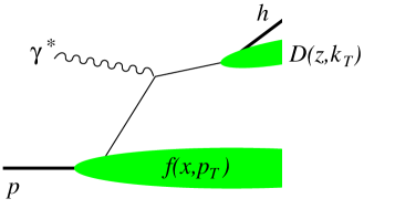
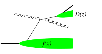
$\mathbf{(a)}$                                                                $\mathbf{(b)}$

Figure 1: The low-$q_{T}$ description $\mathbf{(a)}$ and the high-$q_{T}$ description $\mathbf{(b)}$ for the transverse-momentum distribution of the produced particle $h$ in semi-inclusive deep inelastic scattering, $ep\to e+h+X$.

2 Insight from power counting

It is natural to ask how these two descriptions are related to each other. A first answer can be obtained from a careful look at the power counting in the region of intermediate transverse momentum, $M\ll q_{T}\ll Q$, where both approaches can be applied. The low-$q_{T}$ approach starts with an expansion in the small parameter $q_{T}/Q$ and involves coefficients depending on $M/q_{T}$, which for $q_{T}\gg M$ can be further expanded in $M/q_{T}$. For an observable $F$ with mass dimension $-2$ one thus has

$$F(q_{T},Q)\;\stackrel{{\scriptstyle q_{T}\ll Q}}{{=}}\;\frac{1}{M^{2}}\,\sum_{\text{twist}~{}n}\,\biggl{[}\frac{q_{T}}{Q}\biggr{]}^{n-2}\,l_{n}\biggl{(}\frac{M}{q_{T}}\biggr{)} \;\stackrel{{\scriptstyle M\ll q_{T}\ll Q}}{{=}}\;\frac{1}{M^{2}}\,\sum_{n,k}l_{n,k}\;\biggl{[}\frac{q_{T}}{Q}\biggr{]}^{n-2}\,\biggl{[}\frac{M}{q_{T}}\biggr{]}^{k}\,.$$ (1)

By contrast, the high-$q_{T}$ approach first expands an observable in $M/q_{T}$, with coefficients that for intermediate $q_{T}$ can be further expanded in $q_{T}/Q$ :

$$F(q_{T},Q)\;\stackrel{{\scriptstyle M\ll q_{T}}}{{=}}\;\frac{1}{M^{2}}\,\sum_{\text{twist}~{}n}\,\biggl{[}\frac{M}{q_{T}}\biggr{]}^{n}\,h_{n}\biggl{(}\frac{q_{T}}{Q}\biggr{)} \;\stackrel{{\scriptstyle M\ll q_{T}\ll Q}}{{=}}\;\frac{1}{M^{2}}\,\sum_{n,k}h_{n,k}\;\biggl{[}\frac{M}{q_{T}}\biggr{]}^{n}\,\biggl{[}\frac{q_{T}}{Q}\biggr{]}^{k-2}\,.$$ (2)

The simultaneous validity of both approaches in the region $M\ll q_{T}\ll Q$ implies $l_{n,k}=h_{k,n}$. The first index $n\geq 2$ in each expansion characterizes the twist of the corresponding calculation. In practice only terms with $n=2$ and possibly $n=3$ can actually be calculated.

For observables with nonzero $l_{2,2}=h_{2,2}$, the leading terms in the two calculations coincide for intermediate $q_{T}$, where they provide complementary descriptions of the same physics. One may then try to construct a smooth interpolation between the two descriptions that is valid at all $q_{T}$. There are, however, observables with $l_{2,2}=h_{2,2}=0$, where the leading term $l_{2,4}$ of the low-$q_{T}$ result is distinct from the leading term $h_{2,4}$ of the high-$q_{T}$ result. With both calculations only performed at leading-twist accuracy, one can then add their results at intermediate $q_{T}$ without double counting; which of them is more important at given $q_{T}$ depends on the relative size of $q_{T}/Q$ and $M/q_{T}$. We will encounter examples for both cases in section 4.

3 Structure functions for semi-inclusive deep inelastic scattering

To describe the kinematics we use the standard scaling variables $x$ and $z$, the inelasticity $y$, the photon virtuality $Q$, the scaled transverse momentum $q_{T}=P_{h\perp}/z$ of the produced hadron in the $\gamma^{*}p$ c.m., and the azimuthal angle $\phi$ between the lepton and hadron planes in that frame. Precise definitions are given in [1]. The unpolarized cross section can then be parameterized in the form

$$\frac{d\sigma(ep\to ehX)}{d\phi\,dq_{T}^{2}\,dx\,dy\,dz}=\text{(kin.~{}factor)}\times\Bigl{[}F_{T}+\varepsilon F_{L}+\sqrt{2\varepsilon(1+\varepsilon)}\cos\phi\,F^{\cos\phi}+\varepsilon\cos 2\phi\,F^{\cos 2\phi}\Bigr{]}\,,$$ (3)

where the ratio of longitudinal and transverse photon flux is given by $\varepsilon=(1-y)/(1-y+y^{2}/2)$ in the Bjorken limit. The semi-inclusive structure functions $F_{\ldots}$ depend on $x$, $z$, $q_{T}^{2}$, $Q^{2}$, and the subscripts $T$ and $L$ are respectively associated with transverse and longitudinal photon polarization.

3.1 High-$q_{T}$ calculation

The high-$q_{T}$ calculation gives the structure functions as convolutions

$$F_{\ldots} =\frac{1}{Q^{2}\mskip 1.5muz^{2}}\;\sum_{i,j=q,\,\bar{q},\,g}\;\int_{x}^{1}\frac{d\hat{x}}{\hat{x}}\,\int_{z}^{1}\frac{d\hat{z}}{\hat{z}}\,f_{1}^{i}\Bigl{(}\frac{x}{\hat{x}}\Bigr{)}\,D_{1}^{j}\Bigl{(}\frac{z}{\hat{z}}\Bigr{)}\,K^{ij}_{\ldots}\Bigl{(}\hat{x},\hat{z},\frac{q_{T}}{Q}\Bigr{)}$$ (4)

in longitudinal momentum fractions, where $f_{1}^{i}$ and $D_{1}^{j}$ respectively denote the usual unpolarized collinear distribution and fragmentation functions, and the $K^{ij}_{\ldots}$ are perturbatively calculable hard-scattering kernels. Expanding these kernels in $q_{T}/Q$, one readily obtains the result of the high-$q_{T}$ mechanism for intermediate $q_{T}$. At order $\alpha_{s}$, all structure functions in (3) contain a term proportional to $f_{1}(x)\,D_{1}(z)\,\log(Q/q_{T})$ after this expansion. Higher orders provide terms going like $\alpha_{s}^{n}\log{}^{2m-1}(Q/q_{T})$ with $m\leq n$. To obtain a stable perturbative result in the region where $\log(Q/q_{T})$ is large, these logarithms should be resummed to all orders. We will come back to this in sect. 3.2.

3.2 Low $q_{T}$

In the low-$q_{T}$ description, factorization is fairly well understood at twist-two accuracy [5, 6] and leads to a representation of the form

$$F_{\ldots}=\sum_{i=q,\,\bar{q}}\,xe_{i}^{2} \int d^{2}\vec{p}_{T}\,d^{2}\vec{k}_{T}\,d^{2}\vec{l}_{T}\,\delta(\vec{p}_{T}-\vec{k}_{T}+\vec{l}_{T}+\vec{q}_{T})\,w_{\ldots}(\vec{p}_{T},\vec{k}_{T})\,f^{i}(x,p_{T}^{2})\,D^{i}(z,k_{T}^{2})\,U({l}_{T}^{2})$$ (5)

with known functions $w_{\ldots}\mskip 1.5mu$, where for simplicity I have omitted a hard factor representing $\alpha_{s}$ corrections from virtual graphs. In addition to transverse-momentum dependent distribution and fragmentation functions $f^{i}(x,p_{T}^{2})$ and $D^{i}(z,k_{T}^{2})$, the expression (5) contains a soft factor $U(l_{T}^{2})$ describing soft gluon exchange between partons moving in the direction of the target and partons moving in the direction of the observed hadron $h$. At twist-three accuracy, soft gluon exchange has not been analyzed, so that we do not have a full understanding of factorization for structure functions going like $1/Q$. However, there are detailed calculations at tree level [8, 9], which give results very similar in form to (5) without the factor $U(l_{T}^{2})$.

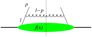
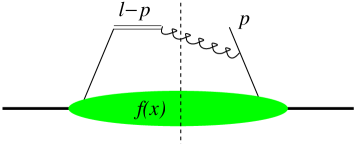
$\mathbf{(a)}$                                                                $\mathbf{(b)}$

Figure 2: Example graphs for the calculation of an unintegrated parton distribution at high $p_{T}$ in terms of a collinear distribution $f(x)$ and a hard-scattering subprocess. The double line represents an eikonal propagator, which comes from the Wilson line $P\exp\bigl{[}-ig\int_{0}^{\infty}d\lambda\,n\cdot A(\xi+\lambda n)\bigr{]}$ in the definition of the parton density [5, 6, 7].

To evaluate (5) for intermediate $q_{T}$, one notes that for $q_{T}\gg M$ at least one of the momenta $p_{T}$, $k_{T}$ or $l_{T}$ has to be large. In this region, the corresponding factor can be calculated using collinear factorization, with the large transverse momentum generated by perturbative parton radiation as illustrated in Fig. 2. As shown in [1], general symmetry considerations allow one to determine the power behavior at high $p_{T}$ for the different parton densities parameterizing the spin and momentum dependence of the quark distribution in a proton. In particular one finds

$$f_{1}(x,p_{T}^{2}) \sim\frac{1}{p_{T}^{2}}\,\alpha_{s}\,\sum_{i=q,\,\bar{q},\,g}\,[f_{1}^{i}\otimes K_{1}^{i}]\,,\qquad\qquad xf^{\perp}(x,p_{T}^{2})\sim\frac{1}{p_{T}^{2}}\,\alpha_{s}\,\sum_{i=q,\,\bar{q},\,g}\,[f_{1}^{i}\otimes K^{\perp i}]\,,$$

$$h_{1}^{\perp}(x,p_{T}^{2}) \sim\frac{M^{2}}{p_{T}^{4}}\,\alpha_{s}\;\sum_{i}\,[\text{collinear twist-three distributions}\otimes K_{3}^{i}]\,,$$ (6)

where $K_{1}^{i}$, $K^{\perp i}$, and $K_{3}^{i}$ are calculable hard-scattering kernels and $\otimes$ denotes a convolution in longitudinal momentum fractions. The Boer-Mulders function $h_{1}^{\perp}$ describes the distribution of transversely polarized quarks in an unpolarized proton, whereas $f^{\perp}$ is a distribution of twist three (involving one good and one bad light-cone component of the quark field). Explicit calculation of $f_{1}(x,p_{T}^{2})$ and $f^{\perp}(x,p_{T}^{2})$ reveals the rapidity divergences discussed in [7]. They have the form

$$\frac{1}{(l-p)\cdot n}=\frac{1}{n^{-}}\,\frac{1}{(l-p)^{+}+\frac{n^{+}}{n^{-}}\,(l-p)^{-}}\qquad\qquad\text{with}~{}~{}~{}(l-p)^{-}=\frac{\vec{p}_{T}^{2}}{2(l-p)^{+}}$$ (7)

and come from the Wilson line in Fig. 2b, or equivalently from the gluon propagator in Fig. 2a if one uses the gauge $n\cdot A=0$ where the Wilson line is unity. In a parton density for a fast right-moving proton, the loop variable $l^{+}$ is integrated down to its lower kinematic limit $p^{+}$. To avoid a logarithmic divergence in (7) one must hence keep $n^{+}$ nonzero (complications arising for spacelike $n$ are discussed in [1, 7]). The light-cone gauge $A^{+}=0$ or a purely lightlike Wilson line cannot be used in this context. It should be instructive to investigate how this affects formulations of QCD based on light-cone gauge. Note that in the context of light-cone quantization, configurations with $(l-p)^{+}=0$ in Fig. 2a correspond to zero modes of the gluon field.

Keeping $n^{+}$ finite in (7) cuts off the region of negative gluon rapidities, where $(l-p)^{+}\to 0$ and $(l-p)^{-}\to\infty$. This is physically reasonable, since fast left-moving gluon modes should not be included in the parton distribution of a fast right-moving hadron. The dependence of unintegrated parton distributions on $n^{+}/n^{-}$ is described by the Collins-Soper equation [5], whose solution can be written as the product of an $n^{+}/n^{-}$ independent initial condition and a Sudakov factor.

Power laws analogous to those in (3.2) are obtained for the fragmentation functions $D_{1}(z,k_{T}^{2})$, $D^{\perp}(z,k_{T}^{2})$, and the Collins function $H_{1}^{\perp}(z,k_{T}^{2})$. Together with the perturbative expression for $U(l_{T}^{2})$ at high $l_{T}$ one can then determine the behavior of the semi-inclusive structure functions for $M\ll q_{T}\ll Q$. The terms going with $n^{+}/n^{-}$ in the distribution and fragmentation functions give rise to a $\log(Q/q_{T})$ in the structure functions, which we also encountered in the high-$q_{T}$ calculation. The Collins-Soper equation allows one to resum such logarithms to all orders and is at the origin of the CSS formalism [10], which plays a prominent role in collider phenomenology. The need to keep $n^{+}/n^{-}$ finite in (7) is thus not a mere technicality but has practical implications for physical observables.

4 Comparing the low- and high-$q_{T}$ calculations

	low-$q_{T}$ calculation			high-$q_{T}$ calculation
	power	twist	contributing functions	power	twist
$F_{T}\sim$	${1}/{q_{T}^{2}}$	2	$f_{1}(x,p_{T}^{2}),D_{1}(z,k_{T}^{2})$	${1}/{q_{T}^{2}}$	2
$F_{L}\sim$	${1}/{Q^{2}}$	4	result unknown	${1}/{Q^{2}}$	2
$F^{\cos 2\phi}\sim$	${M^{2}}/{q_{T}^{4}}\phantom{+}$	2	$h_{1}^{\perp},H_{1}^{\perp}$	${1}/{Q^{2}}$	2
	$+{1}/{Q^{2}}$	4	result unknown
$F^{\cos\phi}\sim$	${1}/{(Q\mskip 1.5muq_{T})}$	3	$f_{1},f^{\perp},D_{1},D^{\perp}$	${1}/{(Q\mskip 1.5muq_{T})}$	2

Table 1: Behavior of semi-inclusive structure functions in the intermediate region $M\ll q_{T}\ll Q$.

The behavior for $M\ll q_{T}\ll Q$ of the unpolarized structure functions obtained in the low- and high-$q_{T}$ calculations is given in Table 1. Explicit evaluation shows that for $F_{T}$ the results of the two calculations exactly coincide; this is an example of the case where at intermediate $q_{T}$ the leading term in the expansions (1) and (2) goes with $l_{2,2}=h_{2,2}$. The agreement between the two calculations can be seen at the level of diagrams: roughly speaking, the graph of Fig. 1b corresponds to the graph in Fig. 3a if the gluon moves fast in the direction of the hadron $h$, and to the graph in Fig. 3b if the gluon moves fast in the direction of the target.

The leading term in the low-$q_{T}$ result for $F^{\cos 2\phi}$ involves the Boer-Mulders and Collins functions. This structure function provides an example for the case where $l_{2,2}=h_{2,2}=0$ and where the leading contributions $l_{2,4}$ and $h_{4,2}$ in the two calculations are different and can be added at intermediate $q_{T}$. From power counting it is clear that the $1/Q^{2}$ behavior obtained in the high-$q_{T}$ calculation for both $F^{\cos 2\phi}$ and $F_{L}$ corresponds to twist-four contributions in the low-$q_{T}$ framework, whose computation is well beyond the state of the art. As a consequence, one cannot invoke the CSS method [10] to resum the logarithms in $Q/q_{T}$ that appear in the high-$q_{T}$ result. Terms going like $1/Q^{2}$ are obtained if one calculates $F_{L}$ and $F^{\cos 2\phi}$ in the parton model [2], considering the graph in Fig. 1a with only the functions $f_{1}(x,p_{T}^{2})$ and $D_{1}(z,k_{T}^{2})$. However, the results do not match with the high-$q_{T}$ calculation at intermediate $q_{T}$ and can hence only be regarded as partial evaluations of the complete (unknown) twist-four terms.

If we perform the twist-three calculation for $F^{\cos\phi}$ at low $q_{T}$ using the tree-level result of [8] supplemented with the soft factor $U(l_{T}^{2})$ of the twist-two factorization formula (5), we obtain agreement with the high-$q_{T}$ result for intermediate $q_{T}$ except for a missing term proportional to $f_{1}(x)\,D_{1}(z)$. Such a term comes from kinematics where both the plus- and the minus-momentum of the gluon in Fig. 3 is negligible. This shows that, if a proper factorization formula for twist three can be established, the soft-gluon sector will have to be treated with particular care.

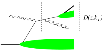
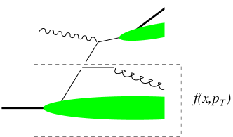
$\mathbf{(a)}$                                                                $\mathbf{(b)}$

Figure 3: Example graphs for the low-$q_{T}$ calculation in the region $q_{T}\gg M$, where a factorized description as in Fig. 2 is valid for the fragmentation function $\smash{\mathbf{(a)}}$ or the parton distribution $\smash{\mathbf{(b)}}$.

5 Summary

The descriptions of transverse-momentum spectra based either on intrinsic transverse momentum of partons or on perturbative radiation are not disconnected. They can be related in an intermediate region $M\ll q_{T}\ll Q$ by describing transverse-momentum dependent distribution and fragmentation functions themselves in terms of perturbative radiation, as indicated in Fig. 2. Understanding the connection between the two approaches for a given observable enables one to devise descriptions that may be used in the full region of $q_{T}$. As shown in [1], the interplay of the two mechanisms has also nontrivial consequences in observables that are integrated over $q_{T}$.

A varied picture arises already for the angular distribution of the measured hadron in unpolarized semi-inclusive scattering, with the results obtained at leading-power accuracy in the low- and high-$q_{T}$ calculations coinciding for some observables but not for others. An even richer phenomenology emerges if one includes polarization effects [1, 11].

The calculation of unintegrated parton densities or fragmentation functions at perturbatively large transverse momenta leads to divergences from gluonic zero modes if naively performed in light-cone gauge. Proper regularization of these divergences physically ensures that left-moving gluon modes are not included in distribution or fragmentation functions for right-moving hadrons and provides a powerful method for resumming logarithms of $Q/q_{T}$ into a Sudakov factor. It remains to be understood how this physics can be treated within light-cone quantization.

References

- [1] A. Bacchetta, D. Boer, M. Diehl and P. J. Mulders, JHEP 0808 (2008) 023 [arXiv:0803.0227].
-
[2]
R. N. Cahn,
Phys. Lett. B 78 (1978) 269;
Phys. Rev. D 40 (1989) 3107;
M. Anselmino, M. Boglione, U. D’Alesio, A. Kotzinian, F. Murgia and A. Prokudin, Phys. Rev. D 71 (2005) 074006 [hep-ph/0501196]. -
[3]
H. Georgi and H. D. Politzer,
Phys. Rev. Lett. 40 (1978) 3;
A. Méndez, A. Raychaudhuri and V. J. Stenger, Nucl. Phys. B 148 (1979) 499;
A. König and P. Kroll, Z. Phys. C 16 (1982) 89;
J. G. Chay, S. D. Ellis and W. J. Stirling, Phys. Rev. D 45 (1992) 46;
P. M. Nadolsky, D. R. Stump and C. P. Yuan, Phys. Lett. B 515 (2001) 175 [hep-ph/0012262]. -
[4]
K. A. Oganesian, H. R. Avakian, N. Bianchi and P. Di Nezza,
Eur. Phys. J. C 5 (1998) 681
[hep-ph/9709342];
M. Anselmino, M. Boglione, A. Prokudin and C. Türk, Eur. Phys. J. A 31 (2007) 373 [hep-ph/0606286];
U. D’Alesio and F. Murgia, Prog. Part. Nucl. Phys. 61 (2008) 394 [arXiv:0712.4328]. - [5] J. C. Collins and D. E. Soper, Nucl. Phys. B 193 (1981) 381, Erratum ibid. B 213 (1983) 545.
-
[6]
X. D. Ji, J. P. Ma and F. Yuan,
Phys. Rev. D 71 (2005) 034005
[hep-ph/0404183];
J. C. Collins, T. C. Rogers and A. M. Stasto, Phys. Rev. D 77 (2008) 085009 [arXiv:0708.2833]. - [7] J. Collins, these proceedings [arXiv:0808.2665].
-
[8]
P. J. Mulders and R. D. Tangerman,
Nucl. Phys. B 461 (1996) 197,
Erratum ibid. B 484 (1997) 538
[hep-ph/9510301];
A. Bacchetta, M. Diehl, K. Goeke, A. Metz, P. J. Mulders and M. Schlegel, JHEP 0702 (2007) 093 [hep-ph/0611265]. - [9] D. Boer, P. J. Mulders and F. Pijlman, Nucl. Phys. B 667 (2003) 201 [hep-ph/0303034].
- [10] J. C. Collins, D. E. Soper and G. Sterman, Nucl. Phys. B 250 (1985) 199.
-
[11]
X. Ji, J. W. Qiu, W. Vogelsang and F. Yuan,
Phys. Lett. B 638 (2006) 178
[hep-ph/0604128];
Y. Koike, W. Vogelsang and F. Yuan, Phys. Lett. B 659 (2008) 878 [arXiv:0711.0636].