Accurate universal models for the mass accretion histories and concentrations of dark matter halos

Abstract

A large amount of observations have constrained cosmological parameters and the initial density fluctuation spectrum to a very high accuracy. However, cosmological parameters change with time and the power index of the power spectrum varies with mass scale dramatically in the so-called concordance $\Lambda$CDM cosmology. Thus, any successful model for its structural evolution should work well simultaneously for various cosmological models and different power spectra.

We use a large set of high-resolution $N$-body simulations of a variety of structure formation models (scale-free, standard CDM, open CDM, and $\Lambda$CDM) to study the mass accretion histories, the mass and redshift dependence of concentrations and the concentration evolution histories of dark matter halos. We find that there is significant disagreement between the much-used empirical models in the literature and our simulations. Based on our simulation results, we find that the mass accretion rate of a halo is tightly correlated with a simple function of its mass, the redshift, parameters of the cosmology and of the initial density fluctuation spectrum, which correctly disentangles the effects of all these factors and halo environments. We also find that the concentration of a halo is strongly correlated with the universe age when its progenitor on the mass accretion history first reaches 4% of its current mass. According to these correlations, we develop new empirical models for both the mass accretion histories and the concentration evolution histories of dark matter halos, and the latter can also be used to predict the mass and redshift dependence of halo concentrations. These models are accurate and universal: the same set of model parameters works well for different cosmological models and for halos of different masses at different redshifts, and in the $\Lambda$CDM case the model predictions match the simulation results very well even though halo mass is traced to about 0.0005 times the final mass, when cosmological parameters and the power index of the initial density fluctuation spectrum have changed dramatically. Our model predictions also match the PINOCCHIO mass accretion histories very well, which are much independent of our numerical simulations and of our definitions of halo merger trees. These models are also simple and easy to implement, making them very useful in modeling the growth and structure of dark matter halos. We provide appendices describing the step-by-step implementation of our models. A calculator which allows one to interactively generate data for any given cosmological model is provided at http://www.shao.ac.cn/dhzhao/mandc.html, together with a user-friendly code to make the relevant calculations and some tables listing the expected concentration as a function of halo mass and redshift in several popular cosmological models. We explain why $\Lambda$CDM and open CDM halos on nearly all mass scales show two distinct phases in their mass growth histories. We discuss implications of the universal relations we find in connection to the formation of dark matter halos in the cosmic density field.

1. Introduction

In the current cold dark matter (CDM) paradigm of structure formation, a key concept in the buildup of structure in the universe is the formation of dark matter halos. These halos are quasi-equilibrium systems of CDM particles formed through nonlinear gravitational collapse in the cosmic density field. Since galaxies and other luminous objects are believed to form by cooling and condensation of the baryonic gas in potential wells of dark matter halos, the understanding of the formation and properties of CDM halos is an important part of galaxy formation.

One of the most important properties of the halo population is their density profiles. Based on $N$-body simulations, Navarro, Frenk, & White (1997, hereafter NFW) found that CDM halos can in general be approximated by a two-parameter profile,

$$\rho(r)=\frac{4\rho_{s}}{(r/R_{s})\left(1+r/R_{s}\right)^{2}}\,,$$ (1)

where $R_{s}$ is a characteristic “inner” radius at which the logarithmic density slope is $-2$, and $\rho_{s}$ is the density at $R_{s}$. A halo is often defined so that the mean density $\rho_{h}$ within the halo radius $R_{h}$ is a factor $\Delta_{h}$ times the mean density of the universe (${\bar{\rho}}$) at the redshift ($z$) in consideration. The halo mass can then be written as

$$M_{h}\equiv\frac{4\pi}{3}\Delta_{h}{\bar{\rho}}R_{h}^{3}\,.$$ (2)

One can define the circular velocity of a halo as $V_{h}=(GM_{h}/R_{h})^{1/2}$, so that

$$M_{h}={V_{h}^{2}R_{h}\over G}={2^{1/2}V_{h}^{3}\over[\Delta_{h}\Omega_{m}(z)]^{1/2}H(z)}\,,$$ (3)

where $H(z)$ is the Hubble parameter and $\Omega_{m}(z)$ is the cosmic mass density parameter at redshift $z$. The shape of an NFW profile is usually characterized by a concentration parameter $c$, defined as $c\equiv R_{h}/R_{s}$. It is then easy to show that

$$\rho_{s}=\rho_{h}\frac{c^{3}}{12\left[\ln(1+c)-c/(1+c)\right]}\,.$$ (4)

We denote the mass within $R_{s}$ by $M_{s}$, and the circular velocity at $R_{s}$ by $V_{s}$. These quantities are related to $c$ and $M_{h}$ by

$$M_{s}={\ln 2-1/2\over\ln(1+c)-c/(1+c)}M_{h}\,,~{}~{}~{}~{}~{}V_{s}^{2}=V_{h}^{2}{cM_{s}\over M_{h}}\,.$$ (5)

In the literature, a number of definitions have been used for $\Delta_{h}$ (hence $R_{h}$). Some authors opt to use $\Delta_{h}=200$ (e.g., Jenkins et al. 2001) or $\Delta_{h}=200/\Omega_{m}(z)$ (e.g., NFW), while others (e.g., Bullock et al. 2001; Jing & Suto 2002) choose $\Delta_{h}=\Delta_{\rm vir}$ according to the spherical virialization criterion (Kitayama & Suto 1996; Bryan & Norman 1998). These different definitions can lead to sizable differences in $c$ for a given halo, and the differences are cosmology-dependent. In our discussion in the main text we use $\Delta_{h}=\Delta_{\rm vir}$, and adopt the fitting formulae of $\Delta_{\rm vir}$ obtained by Bryan & Norman (1998). The value of $\Delta_{\rm vir}$ ranges from $\sim 180$ at high redshift to $\sim 340$ at present for the current ‘concordance’ $\Lambda$CDM cosmology. In appendices A and B, we also provide results based on the other two definitions of $\Delta_{h}$. To avoid confusing, we denote halo mass, radius, concentration and circular velocity by $M$, $R$, $c$, and $V$ for the last definition ($\Delta_{h}=\Delta_{\rm vir}$), by $M_{\rm 200c}$, $R_{\rm 200c}$, $c_{\rm 200c}$, and $V_{\rm 200c}$ for the second definition ($\Delta_{h}=200/\Omega_{m}(z)$), and by $M_{\rm 200m}$, $R_{\rm 200m}$, $c_{\rm 200m}$, and $V_{\rm 200m}$ for the first definition ($\Delta_{h}=200$).

The structure of a halo is expected to depend not only on cosmology and fluctuation power spectrum, but also on its formation history. Attempts have therefore been made to relate the halo concentration to quantities that characterize the formation of the halo. In their original paper, NFW suggested that the characteristic density of a halo, $\rho_{s}$, is a constant ($k$) times the mean density of the universe, ${\bar{\rho}(z_{f})}$, at the redshift $z_{f}$ (referred to as the formation time of the halo by NFW) where half of the halo’s mass was first assembled into progenitors more massive than $f$ times the halo mass. NFW used the extended Press–Schechter formula to calculate $z_{f}$ and found that the anticorrelation between $c$ and $M$ observed in their simulation can be reproduced reasonably well with a proper choice of values of the parameters $k$ and $f$.

Subsequent investigations demonstrated that additional complexities are involved in the CDM halo structure. First, halos of a fixed mass may have significant scatter in their $c$ values (e.g., Jing 2000), although there is a mean trend of $c$ with $M$. If this trend is indeed due to a correlation between concentration and formation time, the scatter in $c$ may reflect the expected scatter in the formation history for halos of a given mass (e.g., Jing 2000, Lu et al. 2006). Second, Bullock et al. (2001, hereafter B01) and Eke et al. (2001, hereafter E01) found that the halo concentration at a fixed mass is systematically lower at higher redshift. B01 proposed a model with $c\propto(M/M_{\star})^{-0.13}/(1+z)$ ($M_{\star}$ being the mass at which the rms of the linear density field is $\sim 1$), which has a stronger halo-mass dependence, and a much stronger redshift dependence, than that predicted by the NFW model. E01 proposed a similar model that has a weaker mass dependence, and a slightly weaker redshift dependence, than the B01 model. Both of these models have been widely used in the literature to predict the concentration–halo mass relation. Using the same set of numerical simulations as that used in B01, Wechsler et al. (2002; hereafter W02) found that, over a large mass range, the mass accretion histories (hereafter MAHs) of individual halos identified at redshift $z_{\rm obs}$ can be approximated by a one-parameter exponential form,

$$M(z)=M(z_{\rm obs}){\rm exp}[-2(z-z_{\rm obs})/(1+z_{f})]\,,$$ (6)

where $z_{f}$ is the formation time of a halo, determined by fitting the simulated MAH with the above formula. Assuming that $c$ equals $4.1$ at $z_{f}$ and grows proportionally to the scale factor $a\propto 1/(1+z)$, W02 proposed a recipe to predict $c$ for individual halos through their MAHs, and found that their model can reproduce the dependence of $c$ on both halo mass and redshift found in B01. Using a large set of Monte Carlo realizations of the extended Press–Schechter formalism (EPS), van den Bosch (2002) showed that the average MAH of CDM halos follows a simple universal function with two scaling variables. Based on a set of high-resolution $N$-body simulations, Zhao et al. (2003a, 2003b, hereafter Z03a and Z03b, respectively) found that the MAH of a halo in general consists of two distinct phases: an early fast phase and a late slow phase (see also Li et al. 2007 and Hoffman et al. 2007). As shown in Z03a, the early phase is characterized by rapid halo growth dominated by major mergers, which effectively reconfigure and deepen the gravitational potential wells and cause the collisionless dark matter particles to undergo dynamical relaxation and mix up sufficiently to form the core structure, while the late phase is characterized by slower quiescent growth predominantly through accretion of material onto the halo outskirt, little affecting the inner structure and potential. Z03a proposed that the concentration evolution of a halo depends much on its mass accretion rate and the faster the mass grows, the slower the concentration increases. In particular, they predicted that halos which are still in the fast growth regime should all have a similar concentration, $c\sim 4$. Using a combination of $N$-body simulations of different resolutions, Z03b studied in detail how the concentrations of CDM halos depend on halo mass at different redshifts. They confirmed that halo concentration at the present time depends strongly on halo mass, but their results also show marked differences from the predictions of the B01 and E01 models. The mass dependence of halo concentrations becomes weaker at higher redshifts, and at $z>3$ halos with $M>10^{11}h^{-1}{\rm M}_{\odot}$ all have a similar median concentration, $c\sim 4$. While the median concentrations of low-mass halos grow significantly with time, those of massive halos change very little with redshift. These results are in good agreement with the empirical model proposed by Z03a and favored by the Chandra observation of Schmidt & Allen (2007), but are very different from the predictions of the models proposed by B01, E01 and W02. Recently, Gao et al. (2008) and Macció et al. (2008) confirmed the results of Z03b with the use of a large set of simulated halos, suggesting again that the much-used B01 and E01 models need to be revised.

There have been attempts to modify the early empirical models of halo MAH and halo concentration to accommodate the new simulation results. Miller et al. (2006) and Neistein et al. (2006) provided MAH models based on theoretical EPS formalism. With help of the Millennium simulation, Neistein & Dekel (2008) presented a empirical algorithm for constructing halo merger trees, which is significantly better than their previous method based on EPS but fails to reproduce the non-Markov features of merger trees. Moreover, because of the limited resolution of the simulation, this algorithm is tuned to reproduce MAHs within redshift 2.5 for only massive halos. McBride et al. (2009) examined halo MAHs of the Millennium simulation and modeled the scatter among different halos by fitting individual MAHs with a two-parameter function, which was proved to be more accurate than the one-parameter function of W02. Note that both the two models above are restricted to the specific cosmology and the specific fluctuation power spectrum of the Millennium simulation, similar to WMAP1 results. Gao et al. (2008) confirmed the finding of B01 that the NFW prescription overpredicts the halo concentrations at high redshift, and tried to overcome this shortcoming by modifying the definition of halo formation time. However, the revised model still fails to reproduce the evolution of concentrations of galaxy sized halos. Modifying the parameters of the B01 and E01 models can also reduce the discrepancy between these models with simulation results at high masses, but the overly rapid redshift evolution of the concentration remains. Motivated partly by Z03a and Z03b, Macció et al. (2008) presented a model based on some modification of the B01 model, and found that it can reproduce the concentration–mass relation at $z=0$ in their simulations. Unfortunately, their model is not universal, because the normalization of the concentration–mass relation has to be calibrated for each cosmological model and for each redshift and thus the model cannot be used to predict correctly the redshift evolution of halo concentrations. In addition, as we will show below, the model of Macció et al. has the same shortcoming as the original B01 model in that it predicts too steep a concentration–mass relation for halos at high redshift in the current $\Lambda$CDM models and for halos at all redshift in the ‘standard’ CDM model with $\Omega_{m,0}=1$. Thus, all the existing empirical models for the halo concentration can at best provide reliable predictions for dark matter halos in limited ranges of halo mass and redshift (often around $z=0$), and only for some specific cosmological models (according to which the empirical models are calibrated). Clearly, they are insufficient in the era of precision cosmology.

We believe that even though a large amount of observations have constrained cosmological parameters and the initial density fluctuation spectrum to a very high accuracy, cosmological parameters change with time and the power index of the power spectrum varies with mass scale dramatically in the so-called concordance $\Lambda$CDM cosmology and thus any successful model for its structural evolution should work well simultaneously for various cosmological models and different power spectra.

In this paper, we use $N$-body simulations of a variety of structure formation models, including a set of scale-free (SF) models, two $\Lambda$CDM (LCDM) models, the standard CDM (SCDM) model, and an open CDM (OCDM) model, to investigate in detail the MAHs, the mass and redshift dependence of concentrations and the concentration evolution histories of dark matter halos. We show that early empirical models for halo MAHs and concentrations all fail significantly to describe the simulation results. Based on our simulation results, we develop new empirical models for both the MAHs and the concentration evolution histories of dark matter halos, and the latter can also be used to predict the mass and redshift dependence of halo concentrations. These models are accurate and universal, in the sense that the same set of model parameters works well for different cosmological models and for halos of different masses and at different redshifts. These models are also simple and easy to implement, making them very useful in modeling the formation and structure of dark matter halos. Furthermore, the universal relations we find may also provide important insight into the formation processes of dark matter halos in the cosmic density field.

The organization of the paper is as follows. In Section 2, we present the set of $N$-body simulations used in the paper. We describe the simulated MAHs and the corresponding modeling in Section 3. Our modeling of halo concentrations is presented in Section 4. Finally, we discuss and summarize our results in Section 5. We provide appendices describing the step-by-step implementation of our models. A calculator which allows one to interactively generate data for any given cosmological model is provided at http://www.shao.ac.cn/dhzhao/mandc.html, together with a user-friendly code to make the relevant calculations and some tables listing the expected concentration as a function of halo mass and redshift in several currently popular models of structure formation.

2. Numerical simulations and dark matter halos

We use a very large set of cosmological simulations to study the formation and structure of dark matter halos of different masses in different cosmological models. The first subset contains the simulations that were used in Z03b: the then ‘concordance’ $\Lambda$CDM model with density parameter $\Omega_{m,0}=0.3$ and a cosmological constant given by $\Omega_{\Lambda,0}=0.7$. These simulations, labeled as LCDM1–3 in Table 1, were generated with a parallel-vectorized Particle-Particle/Particle-Mesh code (Jing & Suto 2002). The linear power spectrum has a shape parameter $\Gamma=\Omega_{m,0}h=0.20$, and an amplitude specified by $\sigma_{8}=0.9$, where $h$ is the Hubble constant in units of $100\,{\rm km\,s^{-1}}\hbox{\rm Mpc}^{-1}$, and $\sigma_{8}$ is the rms of the linear density field smoothed within a sphere of radius $8\,h^{-1}{\rm Mpc}$ at the present time. We used $256^{3}$ particles for the simulation of boxsize $L=25\,h^{-1}{\rm Mpc}$, and $512^{3}$ particles for the other two simulations, $L=100$ and $300\,h^{-1}{\rm Mpc}$ (see Table 1). The simulations with $L=25\,h^{-1}{\rm Mpc}$ and $100\,h^{-1}{\rm Mpc}$ were evolved by 5000 time steps with a force softening length $\eta$ (the diameter of the S2 shaped particles, Hockney & Eastwood 1981) equal to $2.5h^{-1}{\rm kpc}$ and $10h^{-1}{\rm kpc}$, respectively. In order to examine the dependence on cosmological parameters, we also use simulations for the ‘Standard’ CDM model ($\Omega_{m,0}=1$) and the open CDM model ($\Omega_{m,0}=0.3$, $\Omega_{\Lambda,0}=0$), as described in Jing & Suto (2002, 1998). These are listed as SCDM1, SCDM2 and OCDM1 in Table 1, together with the corresponding model and simulation parameters. In addition, we also use a set of four scale-free (SF) simulations in an Einstein de Sitter universe, with the linear power-law power spectra given by $P(k)\propto k^{n}$. These models are listed as SF1–4 in Table 1 and Figure 1 presents the rms of the linear density field $\sigma(M)$ as a function of the mass scale $M$ for SF1–4 and LCDM1–3.

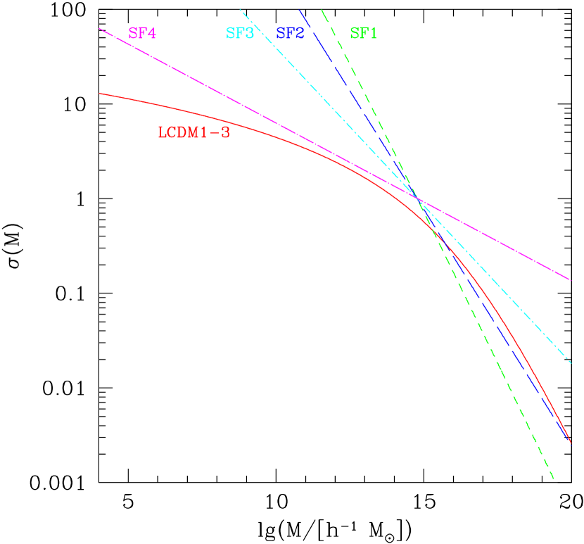
Figure 1.— rms of the linear density fluctuation $\sigma(M)$ as a function of the mass scale $M$ for scale-free simulations with $n=1,\,0,\,-1$, and $-2$, and for $\Lambda$CDM simulations LCDM1–3.

We use both the friends of friends (hereafter FOF) algorithm and the spherical overdensity (hereafter SO) algorithm of Lacey & Cole (1994) to identify dark matter groups in the simulations. The FOF algorithm connects every pair of particles closer than 0.2 times the mean particle distance and the SO algorithm selects spherical regions whose average density is equal to $\Delta_{\rm vir}$ times the mean cosmic density ${\bar{\rho}}$. We select groups at a total of 20–30 snapshots for each CDM simulation and at 10 snapshots for each SF simulation. The outputs are uniformly spaced in the logarithm of the cosmic scale factor $a$. For each group, we choose the particle of the highest local density as the group center, and around it we select as ‘halo’ a spherical region whose average density is $\Delta_{\rm vir}{\bar{\rho}}$, with a routine very similar to the SO algorithm except that here the group center is fixed. We find that the results presented in this paper do not depend significantly on the group finding algorithm. Our following presentation is based on the FOF groups and we use all FOF groups without applying any further selection criteria.

Table 1A Summary of Simulation Parameters

Simulation	$n_{i}$	$h$	$\sigma_{8}$	$\Omega_{m,0}$	$\Omega_{\Lambda,0}$	$N_{p}$	$L[h^{-1}\rm Mpc]$	$N_{NQ}$	$\eta$	$z_{i}$
SF1	1		1	1	0	$512^{3}$	160	512	0.016	1481.3
SF2	0		1	1	0	$512^{3}$	160	512	0.016	363.2
SF3	-1		1	1	0	$512^{3}$	160	512	0.016	75.0
SF4	-2		1	1	0	$512^{3}$	160	512	0.016	11.3
LCDM1	1	0.667	0.9	0.3	0.7	$256^{3}$	25	512	0.0025	72
LCDM2	1	0.667	0.9	0.3	0.7	$512^{3}$	100	512	0.01	72
LCDM3	1	0.667	0.9	0.3	0.7	$512^{3}$	300	512	0.03	36
LCDM4	1	0.71	0.85	0.268	0.732	$1024^{3}$	300	1024	0.01	72
LCDM5	1	0.71	0.85	0.268	0.732	$1024^{3}$	1200	1024	0.072	72
LCDM6	1	0.71	0.85	0.268	0.732	$1024^{3}$	1800	1024	0.144	72
OCDM1	1	0.667	1.0	0.3	0	$256^{3}$	50	256	0.02	72
SCDM1	1	0.5	0.55	1	0	$256^{3}$	25	512	0.0025	72
SCDM2	1	0.5	0.55	1	0	$512^{3}$	100	256	0.02	72
SCDM3	1	0.5	0.55	1	0	$512^{3}$	300	256	0.03	36

The simulations described above are also used to study the density profiles and the concentrations of dark matter halos. We use all halos containing more than 500 particles for our analysis. Each halo is fitted with the NFW profile, using a similar method as described in Z03b. As demonstrated in Z03b, 500 particles are sufficient for measuring the concentration parameter reliably. In order to examine concentrations of very massive halos, we also use three additional simulations with large boxsizes (see Jing, Suto & Mo, 2007). These simulations are listed as LCDM4–6 in Table 1. Note that the model parameters of these simulations are slightly different from those of LCDM1–3. Furthermore, the initial power spectrum for these simulations is obtained using the fitting formula of Eisenstein & Hu (1998), which includes the effects of baryonic oscillations. The details of these simulations can be found in Jing, Suto & Mo (2007), and all the change in model parameters are properly taken into account when we compare our model predictions of halo concentrations with the simulation results. For the same reason, we also use a SCDM simulation of boxsize $L=300\,h^{-1}{\rm Mpc}$ (listed as SCDM3 in Table 1) to investigate the concentration–mass relation at the highest halo mass end in this model.

3. A universal model for the halo mass accretion histories

Since we want to study how a halo grows with time, we need to construct the main branch of the merger tree for each halo. Given a group of dark matter particles at a given output time (which we refer to as group 2), we trace all its particles back to an earlier output time. A group (group 1) at the earlier output is selected as the “main progenitor” of group 2 if it contributes the largest number of particles to group 2 among all groups at this earlier output. We found that in most cases more than half of the particles of group 1 is contained in group 2. We refer to group 2 as the “main offspring” of group 1. We construct the main branch of the merger tree, for each of the most massive 10000 halos identified at redshift $z=0$, until the number of particles in the progenitor drops below 10 or the main progenitor cannot be found anymore. More than $97\%$ of the histories analyzed here can be traced until the particle number goes below 10.

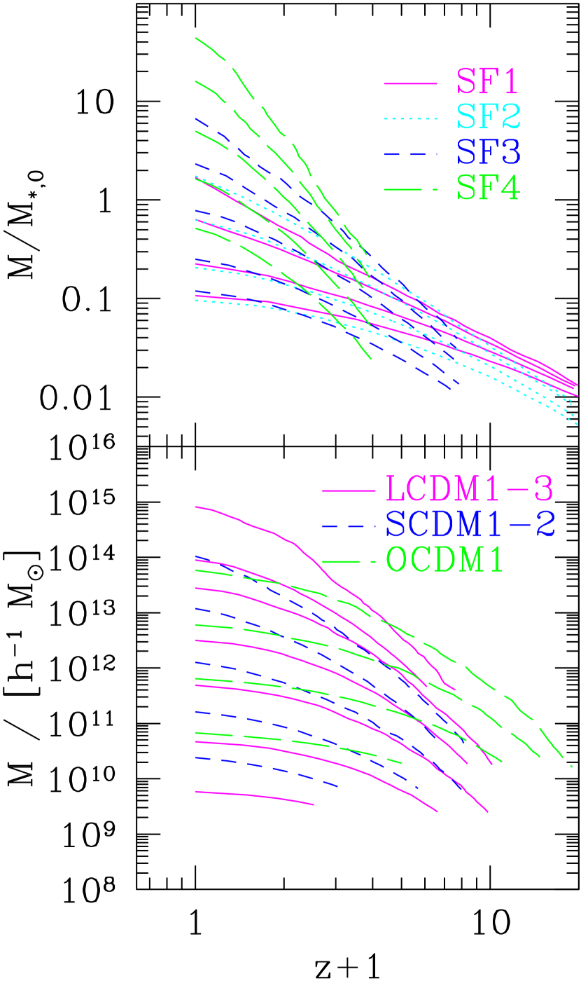
Figure 2.— Median halo MAHs obtained from scale-free simulations with $n=1,\,0,\,-1,$ and $-2$ and from CDM simulations LCDM1–3, SCDM1–2, and OCDM1. Different lines represent median histories with different final halo masses. For each final mass, the result is plotted to a redshift when the histories of $90\%$ of the halos can still be traced.

As an illustration, Figure 2 shows the median MAHs of halos both in the SF simulations and in the CDM models. The halo mass is normalized by the characteristic mass $M_{*,0}$ at the final output in the SF simulations. Clearly, MAHs depend on the power spectrum. This is because halos grow faster in a model with a smaller value of $n$. The effect of cosmological parameters can also be seen clearly in CDM models: the growth of halos is slower in the LCDM model than in the SCDM model (despite the fact that the LCDM has more clustering power than the SCDM) and is the slowest in the OCDM. In our analysis, we have taken into account the incompleteness effect of the MAHs at the earliest epochs when the progenitors containing less than 10 particles cannot be followed in the simulation. This effect leads to an overestimation of MAHs. In order to correct for it, statistical analysis of the MAHs is carried out only up to the redshift where the progenitors of $90\%$ of all the halos in consideration can be traced.

As one can see from Figure 2, the MAHs show a complex dependence on power spectrum, cosmology and halo mass. The goal of this section is to find an order in such complexity so as to obtain a universal model to describe all the MAHs.

3.1. The Expected Asymptotic Behavior at High Redshift

Before modeling the MAHs in detail, let us first consider some generic properties of the growth of CDM halos in the cosmic density field. In the CDM scenario, structures form in a hierarchical fashion, and the growth of dark matter halos in general has the following properties. First, at any given time, more massive halos are, on average, growing faster because they sit in higher density environments. Second, the higher the redshift, the faster the halos of a fixed mass grow because at high redshift they are relatively more massive with respect to others. Third, the MAH of a halo depends on power spectrum of the initial density fluctuation, as mentioned before. Fourth, the MAH of a halo also depends on cosmology, because of the change of the background expansion. The last, halo growth also suffers from some nonlinear processes in their local environments. All these factors entangle together and keep varying in their own complicated ways. For example, in a $\Lambda$CDM universe, the cosmological density parameter $\Omega_{m}$ decrease with time and the power index of the initial density fluctuation spectrum increase with mass scale dramatically, as shown in Figure 3 and Figure 1, respectively. This is why one need a universal evolution model which works well for various cosmologies and different spectra, as mentioned in the introduction already. For exactly the same reason, however, we may not expect that variations of all these factors compensate exactly to bring us a universal function form for MAH in terms of $M$ and $z$. Thus, we turn to model halo mass accretion rate instead, which can be integrated to build the MAH, and in order to describe the accretion rate accurately and universally, we need to disentangle all effects due to halo mass, redshift, the cosmological parameters, the linear power spectrum and those relevant nonlinear processes.

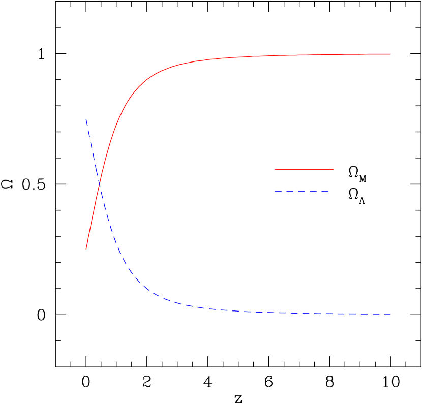
Figure 3.— Evolution of cosmological density parameter $\Omega_{m}$ and cosmological constant parameter $\Omega_{\Lambda}$ for a flat universe with cosmological constant.

Consider two average halos of different masses at a given time. Since the more massive one grows faster, we expect that at a slightly earlier time, the two halos were closer in mass (in terms of the mass ratio), and the masses of their progenitors at higher redshift are expected to be even closer. The two halos are expected to have similar mass accretion rate at sufficiently high redshift, because otherwise with finite difference in accretion rates their mass accretion trajectories would cross. This would lead to an unlikely situation where more massive progenitors actually grow slower than low-mass progenitors at redshifts higher than the crossing redshift. This means that the average MAHs of halos of different masses should all have the same asymptotic behavior at high redshift. Here we try to look for this behavior.

Let us first consider an Einstein de Sitter universe with an initial Gaussian density fluctuation field of a power-law power spectrum, $P(k)\propto k^{n}$. As there is no characteristic scale either in time or in space, this is a case where the structure formation is a self-similar process. When halo mass is scaled with a time-dependent characteristic mass, all statistical quantities as functions of the scaled mass should be the same at all redshifts. Given a linear power spectrum, we can linearly extrapolate to $z=0$, and estimate, the rms of the linear density field $\sigma(M)$ on a mass scale $M$. According to the spherical collapse model, the linear critical overdensity for collapse at redshift $z$ is $\delta_{c}(z)=\delta^{\prime}_{c}[\Omega_{m}(z),\Omega_{\Lambda}(z)]/D(z)$, where $D(z)$ is the linear growth factor, which is $1/(1+z)$ in an Einstein de Sitter universe, and $\delta^{\prime}_{c}[\Omega_{m}(z),\Omega_{\Lambda}(z)]$ is the conventional critical overdensity for collapse at redshift $z$, which is a constant $\cong 1.686$ in this universe. Because $\delta_{c}(z)$ is a function of only $z$ and $\sigma(M)$ is a function of only $M$, we can think of $1/\sigma^{2}(M)$ as the “mass” and $1/\delta^{2}_{c}(z)$ as the “time”. Furthermore, since $M_{\star}$, which satisfies $\sigma(M_{\star})=\delta_{c}(z)$, represents the characteristic nonlinear mass at redshift $z$, $1/\delta^{2}_{c}(z)$ actually corresponds to the characteristic nonlinear “mass” at redshift $z$ if $1/\sigma^{2}(M)$ is regarded as “mass”. In this case, the scaled “mass” is $\nu=\delta^{2}_{c}(z)/\sigma^{2}(M)$, i.e., the peak height of the halo in the conventional terminology.

Suppose that there are some halos at a given redshift $z_{\rm obs}$ and the average mass growth rate is $d\ln\sigma^{2}(M)/d\ln\delta^{2}_{c}(z)|_{z_{\rm obs}}=1$, i.e., $d\ln\nu/d\ln\delta^{2}_{c}(z)|_{z_{\rm obs}}=0$ so that $\nu={\rm constant}$. Then at a slightly higher redshift, $z_{1}$, the scaled mass $\nu$ of their progenitors will be the same as that at $z_{\rm obs}$. Since the statistical properties of halos of the same scaled mass are the same for all redshifts in the self-similar case, these progenitors will have the same growth rate as that at $z_{\rm obs}$, i.e., both the mass growth rate $d\ln\sigma^{2}(M)/d\ln\delta^{2}_{c}(z)|_{z_{\rm obs}}$, and the scaled mass $\nu$, remains constant with time. Therefore, the main progenitors at different redshifts will all have the same $\nu$ and the same growth rate as they have at redshift $z_{\rm obs}$, and the average MAH will be a straight line in the logarithmic diagram of $\sigma$ versus $\delta_{c}$. This line is exactly the asymptotic behavior we are looking for.

In the case of cold dark matter cosmology (SCDM, LCDM, and OCDM), structure formation is not self-similar. Nevertheless, we can still use $1/\sigma^{2}(M)$ to represent halo mass, $1/\delta^{2}_{c}(z)$ to represent time, and $\nu$ to represent the scaled mass. However, it is not guaranteed that the $\sigma$–$\delta_{c}$ relation has a unique asymptotic behavior as it has in the SF case. As we will see below, simulated median MAHs of different final masses show the same asymptotic behavior at high $z$ not only for the SF models but also for the CDM models. We can then use the result to guide our modeling of the halo MAHs in simulations.

3.2. Toward a Universal Model for the Halo Mass Accretion Histories

If we use $1/\sigma(M)$ as mass and $1/\delta_{c}(z)$ as time, the MAH looks like the curves shown in Figure 4, where we have adopted the $n=-1$ SF model as an example. The figure clearly shows the asymptotic behavior described above. The MAHs of halos of different present masses converge at high redshift, and the scaled mass $\sqrt{\nu}=\delta_{c}(z)/\sigma(M)$ approaches a constant, as one can see in the case of the most massive halos in the figure, and as expected from the asymptotic behavior discussed above.

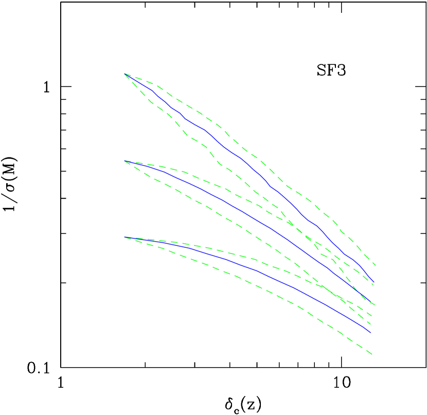
Figure 4.— Median (solid blue) and scatter (dashed green) of the simulated MAHs, in terms of $1/\sigma(M)$ vs. $\delta_{c}(z)$, for halos of three final masses in the scale-free case with $n=-1$. Dashed green lines enclose $60\%$ of the histories in each mass bin.

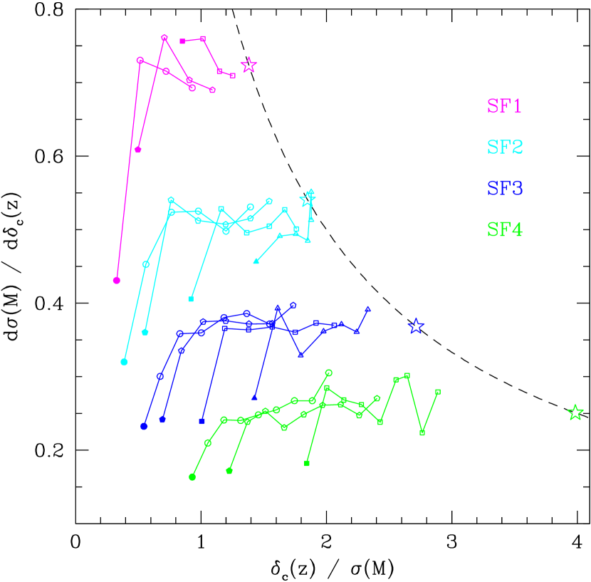
Figure 5.— Median mass accretion rate for our four scale-free models. Purple, blue, dark blue and green symbols and lines represent results for scale-free simulations with $n=1,\,0,\,-1$, and $-2$, respectively. Different symbols represent median histories with different final halo masses, and in each history we use a solid symbol to denote the final snapshot of the history. The four stars and the dashed curve represent the expected asymptotic behavior for high peaks in scale-free models.

Figure 5 shows the median accretion rate, $d\sigma(M)/d\delta_{c}(z)$, as a function of the scaled mass, $\sqrt{\nu}=\delta_{c}(z)/\sigma(M)$, for the four SF models. For each model, a set of symbols of the same type connected with a solid line represents accretion rates of progenitors of the halos of a given mass at $z=0$, and the filled symbol represents the end of the MAH at $z=0$. It is interesting to note that, for each SF model, the results for different halo masses are similar except at the end of the history. The accretion rate plotted in this way is approximately a constant for all the progenitors. As mentioned above, in each model the scaled mass is asymptotically a constant at high $z$. This corresponds to a line, $d\sigma(M)/d\delta_{c}(z)=\sigma(M)/\delta_{c}(z)$, which is plotted as the dashed line in the figure together with a star showing the corresponding asymptotic accretion rate. At the end of each history, the mass accretion rate is somewhat lower than the average of their progenitors. This deviation from self-similarity is not a numerical artifact, as the simulation resolution is sufficient at $z=0$. Instead, it reflects the fact that the main progenitors are a special subset of the total halo population. While the halos of a given $\nu$ at the end of MAHs are chosen only by mass, their progenitors have an additional selection bias: they are chosen to be main progenitors of more massive halos. This biases the progenitor halos to have higher mass accretion rates than typical halos of a given $\nu$ value. In other words, a fraction of halos in the total population are not main progenitors of larger halos in the future but instead will be swallowed by more massive halos. Their mass accretion rates may have been suppressed by their massive neighbors due to environment-heating or tidal-stripping, as envisaged in Wang et al. (2007), and thus their merger trees should also have some non-Markov features.

As seen in Figure 5, accretion rates are different in different SF models, again indicating that the accretion rate depends on the shape of the power spectrum. In order to model such dependence, we use $d\ln\sigma(M)/d\ln\delta_{c}(z)$ instead of $d\sigma(M)/d\delta_{c}(z)$ to represent the accretion rate. The results are shown in the upper left panel of Figure 6, which again indicates that the accretion rate depends strongly on the power index of the linear spectrum. However, we find that this dependence can be scaled away if we use the following variable instead of $\delta(z)/\sigma(M)$:

$$w(z,M)\equiv\delta_{c}(z)/s(M)\,,$$ (7)

where

$$s(M)\equiv\sigma(M)\times 10^{d\lg\sigma/{d\lg m}|_{M}}\,.$$ (8)

This is shown in the upper right panel of Figure 6. With the use of $w(z,M)$, all the halo MAHs lie on top of each other, except for the snapshots close to the end of the MAHs. Even more remarkably, the accretion rates of the progenitors at high redshift can all be well described by a straight line,

$$d\lg\sigma(M)/{d\lg\delta_{c}(z)}=\frac{w(z,M)}{5.85}\,,$$ (9)

which is shown in the panel as the solid line. Note that $\lg s(M)$ is equal to $\lg\sigma(M)$ plus its logarithmic slope at mass $M$: $d\lg\sigma/{d\lg m}|_{M}$. For a given power spectrum with $n>-3$, $\sigma(M)$ decreases with halo mass and so $w(z,M)$ increases with halo mass. The simple relation given by Equation (9) also describes well the MAHs at high redshifts in the LCDM model (see the lower two panels of Figure 6), although the power spectrum and the cosmology are very different from the SF models.

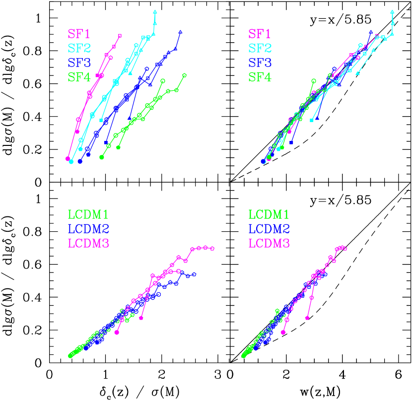
Figure 6.— Same as Figure 5, except that both the horizontal and vertical axes have been rescaled as indicated by the axis labels. Results for the six LCDM histories shown in Figure 2 with final halo mass larger than $10^{10}h^{-1}M_{\odot}$ are also plotted here, in the two lower panels. The black solid straight lines in the right two panels have a slope $1/5.85$, and the dashed curve in each of the two panels represents the envelope given by halos in the end of the MAHs in simulations LCDM1–3.

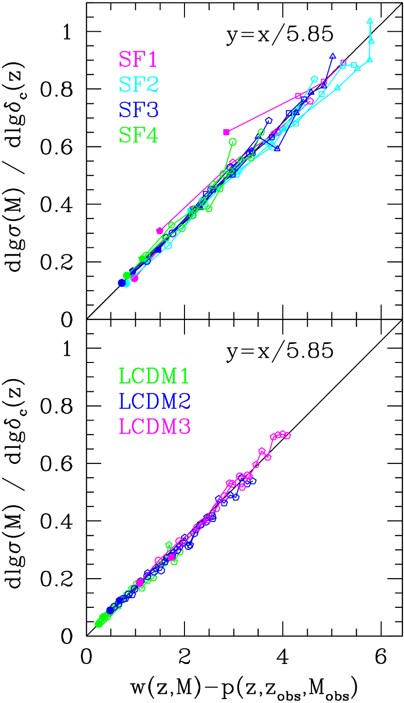
Figure 7.— Same as Figure 6, except that the horizontal axis is rescaled again, as indicated by the axis label. Here $p$ is defined in the text.

As shown in the two right panels of Figure 6, the accretion rate is systematically lower than that given by Equation (9) at the end of the MAHs. We find that this decrease of the accretion rate can be accounted for by replacing $w(z,M)$ with $w(z,M)-p(z,z_{\rm obs},M_{\rm obs})$. The shift, $p(z,z_{\rm obs},M_{\rm obs})$, in the horizontal axis depends on redshift and halo mass in the following way,

$$p(z,z_{\rm obs},M_{\rm obs})=p(z_{\rm obs},z_{\rm obs},M_{\rm obs})$$

$$\times{\rm Max}\left[0,1-\frac{\lg\delta_{c}(z)-\lg\delta_{c}(z_{\rm obs})}{0.272/w(z_{\rm obs},M_{\rm obs})}\right]\,,$$ (10)

where

$$p(z_{\rm obs},z_{\rm obs},M_{\rm obs})=\frac{1}{1+[w(z_{\rm obs},M_{\rm obs})/4]^{6}}\frac{w(z_{\rm obs},M_{\rm obs})}{2}\,$$ (11)

is the shift at $z_{\rm obs}$, the redshift at which the final halo is identified. The horizontal gap between the dashed and solid curves in the right two panels of Figure 6 shows this shift. As one can see, the shift describes well the deviation of the mass accretion rates in the end of the histories (the solid symbols) for the LCDM model. For the SF models, the shift appears to be too much, but this is mainly due to the fact that the interval of the last two snapshots in the SF models is quite big, and the accretion rate is not estimated accurately. Figure 7 shows $d\lg\sigma(M)/{d\lg\delta_{c}(z)}$ versus $w(z,M)-p(z,z_{\rm obs},M_{\rm obs})$. It is clear that the relation is much tighter, and is well described by the following relation,

$$d\lg\sigma(M)/{d\lg\delta_{c}(z)}=\frac{w(z,M)-p(z,z_{\rm obs},M_{\rm obs})}{5.85}\,,$$ (12)

which is shown as the solid lines. The same results are also found for the SCDM and OCDM simulations, although they are not shown here.

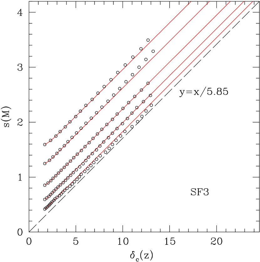
Figure 8.— Predicted and simulated median halo MAHs for the scale-free model with $n=-1$. Black symbols are simulation results, and solid red lines represent our model predictions. Results are shown for halos in five bins of final mass.

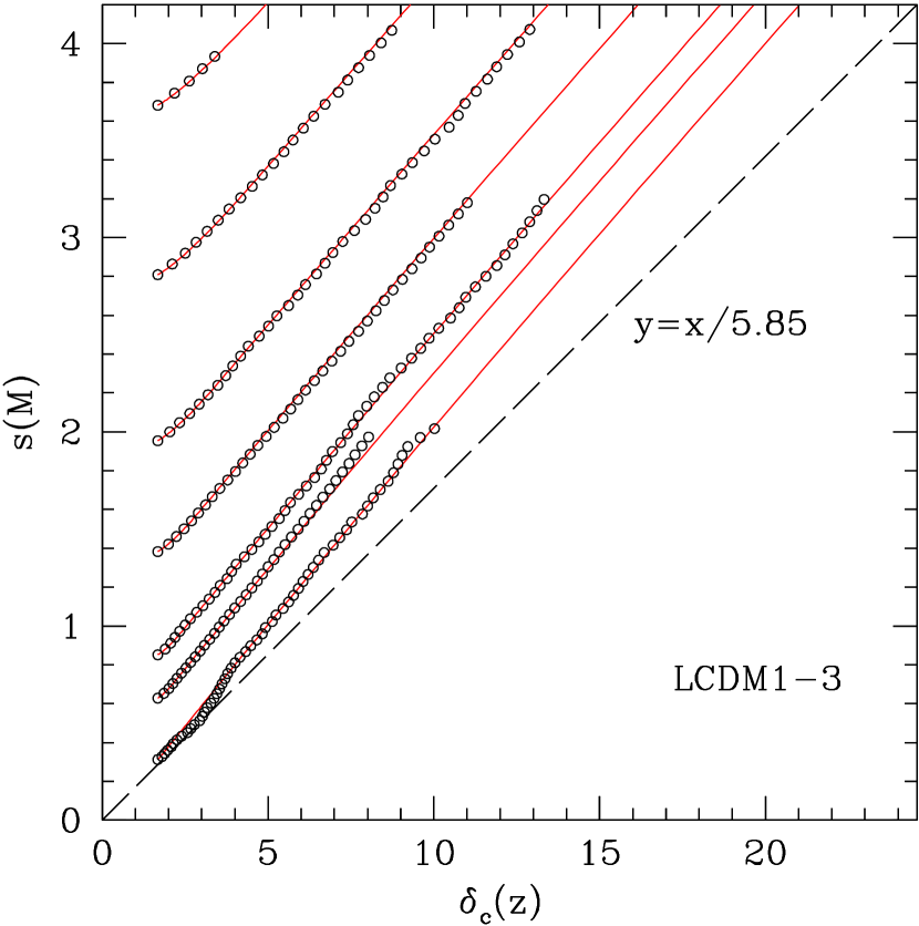
Figure 9.— Predicted and simulated median halo MAHs for simulations LCDM1–3. Symbols and lines are the same as in Figure 8. Here results are shown for halos in seven bins of final mass.

Given a cosmology and a linear power spectrum, it is easy to calculate $s(M)$ for a halo of mass $M_{\rm obs}$ at a given redshift $z_{\rm obs}$. From Equation (12), one can estimate the mass accretion rate, $d\lg\sigma(M)/{d\lg\delta_{c}(z)}$ at $z_{\rm obs}$. One can then compute $\sigma(M)$ [or equivalently $s(M)$] at a redshift $z$ incrementally higher than $z_{\rm obs}$, thus tracing the MAH to higher redshifts. The MAH, in terms of $s(M)$ and $\delta_{c}(z)$, thus computed are shown in Figures 8 and 9. Since $s(M)$ is a monotonic function of $M$ and $\delta_{c}(z)$ a monotonic function of $z$, the $s(M)$–$\delta_{c}(z)$ relation can easily be converted into an MAH in terms of $M$ and $(1+z)$. Figures 10–12 show the median MAHs so obtained for halos of different final masses at different redshifts in various models (solid curves), in comparison with the simulation results (circles). For the $\Lambda$CDM case, the model predictions match the simulation results very well even though halo mass is traced to about 0.0005 times the final mass, when cosmological parameters and the power index of the initial density fluctuation spectrum have changed dramatically. Moreover, the same set model parameters works pretty good for all halo masses, all redshifts and all cosmologies we are studying here. The typical errors of the predicted median MAHs in most cases are $\leq 10\%$. Somewhat larger errors seen in the highest mass bin in Figure 11 may be due to the inaccurate determination in the simulation because the number of halos is small in this mass bin. These predictions are much more accurate than those of the model of W02, shown as the short-dashed lines in Figures 10–12, and those of the model of van den Bosch (2002), shown as the long-dashed lines in Figures 10–12. Furthermore, unlike the latter two models, the MAHs predicted by our model for halos of different final masses do not cross at high redshift. Note that the W02 model works pretty well for low-mass halos in the $\Lambda$CDM and the OCDM models ($M<10^{12}M_{\odot}$). However, for more massive halos in these two models and for all halos in the scale-free and the SCDM simulations, it fails to provide an accurate description for the MAHs. Even though the W02 model and ours give similar MAHs for low-mass halos in some CDM models, they have very different asymptotic behaviors at high redshift, because the W02 model is an exponential function of $z$ while ours is a power-law function of $z$.

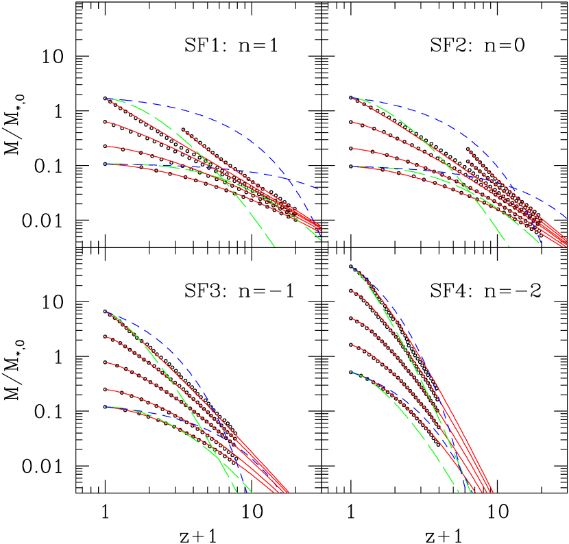
Figure 10.— Predicted and simulated median halo MAHs for scale-free models with $n=1,\,0,\,-1$ and $-2$. Black symbols are simulation results, while solid red lines represent our model predictions. Those histories ended at high redshifts are MAHs with final halos chosen at those redshifts. The short-dashed blue lines and the long-dashed green lines are predictions of the model of W02 and predictions of the model of van den Bosch (2002; based on Monte Carlo realizations of EPS), respectively.

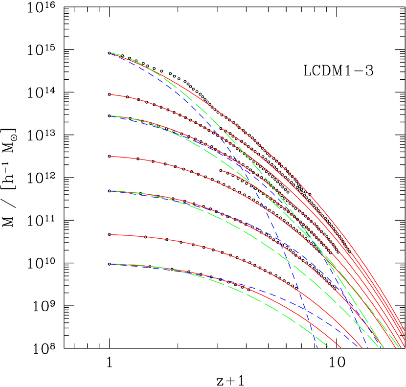
Figure 11.— Predicted and simulated median halo MAHs for simulations LCDM1–3. Symbols and lines are the same as in Figure 10.

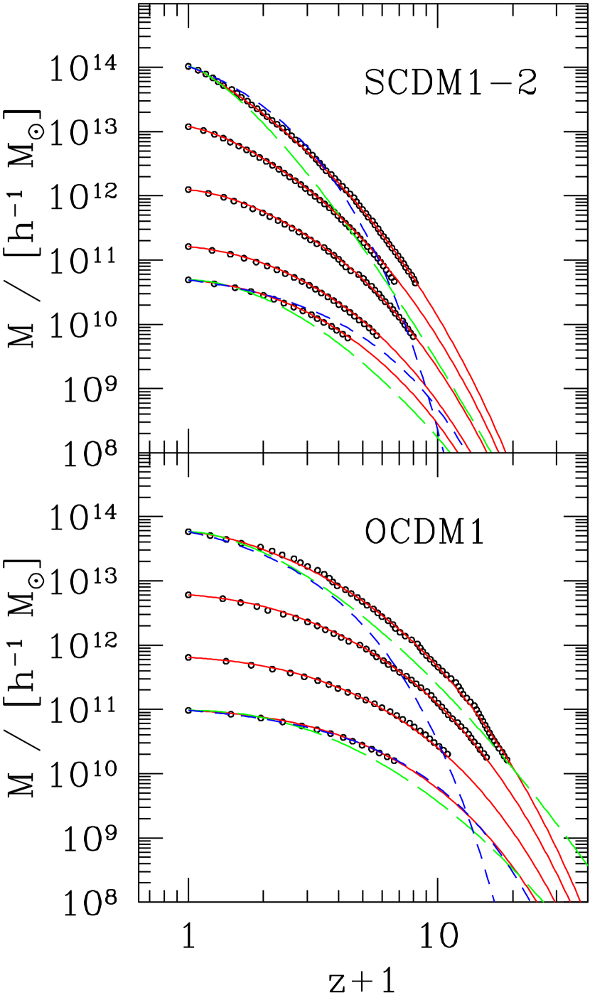
Figure 12.— Predicted and simulated median halo MAHs for simulations SCDM1–2 and OCDM1. Symbols and lines are the same as in Figure 10.

Figure 13.— Predicted and the PINOCCHIO median halo MAHs for a cosmology model the same as LCDM1–3. Black symbols represent the median redshifts of the halo MAHs output by the PINOCCHIO code automatically, while solid red lines are our model predictions. Four different PINOCCHIO runs with box sizes of 25, 100, 300, and $1200\,h^{-1}{\rm Mpc}$ and particle numbers of $256^{3}$, $256^{3}$, $512^{3}$, and $256^{3}$ are analyzed here. The vertical dotted line indicates the redshift 4.

Several months after this current paper was submitted to the Journal and the Internet, McBride et al. (2009) modeled the distribution of halo MAHs of the Millennium simulation by fitting individual MAHs with a two-parameter function, instead of the one-parameter function of W02. They found that our model prediction for the mass accretion rate to have a slightly steeper $z$ dependence than their Equation (9) where our median value is within $20\%$ of their median mass accretion rate at $z\sim 0$ but exceeds theirs by a factor of $\sim 2$ at $z\sim 4$. The reason for this large discrepancy is unknown, however, it is worthy to point out that since we combine a set of high-resolution simulations, the dynamical ranges explored here are larger than the Millennium Simulation and our halo samples are well enough for analyzing the median value. To test our model further, we utilize the Lagrangian semianalytic code PINOCCHIO, proposed by Monaco et al. (2002) for identifying dark matter halos in a given numerical realization of the initial density field in a hierarchical universe. Figure 13 compares our model predictions with the median redshifts of the MAHs produced by the PINOCCHIO code, for a cosmology model the same as LCDM1-3 and very similar to that of the Millennium Simulation. Here four different PINOCCHIO runs with box sizes of 25, 100, 300, and $1200\,h^{-1}{\rm Mpc}$ and particle numbers of $256^{3}$, $256^{3}$, $512^{3}$, and $256^{3}$ are analyzed and, to avoid artifact, only those MAHs which converge among runs of different boxsizes are plotted. Again, at all redshifts available, our model predictions match the median values of the PINOCCHIO MAHs very well in halo mass range probed by the Millennium Simulation. The fluctuations on the median MAHs in the smallest box are due to the small number statistics. Note that the PINOCCHIO MAHs are automatically output by the PINOCCHIO code without any postprocessing and so are much independent of our numerical simulations and of our definitions of halo merger trees.

It is interesting to examine the scaling relations obtained above more closely. At sufficiently high $z$ when $\lg\delta_{c}(z)-\lg\delta_{c}(z_{\rm obs})>0.272/w(z_{\rm obs})$, Equation (3.2) gives $p=0$, and Equation (12) reduces to a simpler form. In this case, $w(z,M)\equiv\delta_{c}(z)/s(M)=5.85$ corresponds to $d\lg\sigma(M)/{d\lg\delta_{c}(z)}=1$, or equivalently to $d\lg\nu/{d\lg\delta^{2}_{c}(z)}=0$. The scaled mass, $\sqrt{\nu}$, is then independent of time, so is $w$ in the SF case. This corresponds to the high-redshift asymptotic behavior discussed in the last subsection. For halos more massive than this characteristic scale, the model predicts that $d\lg\sigma(M)/{d\lg\delta_{c}(z)}>1$ and that $\sqrt{\nu}$ increases with time. For scale-free cases, this means that the most massive halos will grow faster and faster, as demonstrated in the two upper panels of Figure 10, while for $\Lambda$CDM and OCDM cases, this kind of rapidly growing halos are very rare because neither the $\delta_{c}$–$1+z$ relation nor the $\sigma$–$M$ relation is a simple power law. Both the decrease of cosmological density parameter $\Omega_{m}$ with time and the increase of power index of the power spectrum with mass scale will slow down the halo mass growth rate, as shown above. This is why at the present time halos on nearly all mass scales show two distinct phases in their mass growth histories, as found by Z03b and Z03a.

For the SF models, we can obtain some useful analytic formulae, because here $\sigma(M)$ has a simple power-law dependence on $M$: $\sigma\propto M^{-(n+3)/6}$. First, using the high-$z$ asymptote, $w(z,M)=5.85$, we have $\delta_{c}(z)/\sigma(M)=5.85\times 10^{d\lg\sigma/{d\lg m}}=5.85\times 10^{-(n+3)/6}$ and $\nu=5.85^{2}\times 10^{-(n+3)/3}$. This means that the mass of a median progenitor at sufficiently high redshift is a fixed fraction of the characteristic mass: $M=5.85^{6/(n+3)}(M_{*}/10)$. For $n=1,\,0,\,-1$ and $-2$, these progenitors have a typical mass $M/M_{*}=1.415,3.422,20.02$, and $4008.07$, respectively. Second, because $d\lg\sigma/d\lg m=-(n+3)/6$ is a constant in an SF model, we have $d\lg s(M)/{d\lg\delta_{c}(z)}=d\lg\sigma(M)/{d\lg\delta_{c}(z)}=w(z,M)/5.85=\delta_{c}(z)/s(M)/5.85$ when $p(z)=0$. The solution is $s(M)=\delta_{c}(z)/5.85+C$ with $C$ a constant along each median history. This solution describes the MAHs in the SF models quite well, as shown in Figure 8. The $s(M)$–$\delta_{c}(z)$ relations in the CDM models are steeper than that given by this simple model, as shown in Figure 9, because the effective power spectrum index, which comes into the definition of $s(M)$ increases with the mass scale.

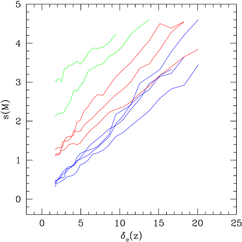
Figure 14.— Simulated mass accretion histories for individual halos in simulations LCDM1–3. For clarity, histories of different final masses are presented with different colors.

Before ending this section, we would like to point out that the scaling relations obtained here may also apply for individual halos. As shown in Figure 14, the linear relation between $s(M)$ and $\delta_{c}(z)$ is also a good approximation for individual halos, although the slope may change from halo to halo. Thus, one may model the individual MAHs using a straight line with its slope changing from halo to halo. The scatter in the MAHs for halos of a given mass may then be modeled through the distribution of the slope. Since the linear relation is a good approximation for different halo masses and in different cosmologies, as shown in Figures 8 and 9, this kind of modeling is expected to be valid for different halos and in different cosmological models. We will come back to this point in a forthcoming paper.

4. A universal model for the dark matter halo concentrations

4.1. The Mass and Redshift Dependence of Halo Concentration

Median values of the halo concentrations measured for the CDM models are plotted as symbols in Figures 15–17. The results obtained here from simulations LCDM1–3 are in excellent agreement with the results obtained in Z03b. In these plots, we also compare our simulation results with the three much-used empirical models. The first one is the NFW model, which relates the halo characteristic density at $R_{s}$ to the universe density at the time when $50\%$ of the halo mass is already in progenitors of $1\%$ of the halo mass or bigger. In agreement with B01, our results show that the NFW model not only fails to predict correctly the redshift dependence of halo concentration, but also fails to predict the concentration at $z=0$ accurately. The model of E01 matches our results better, especially at $z=1$ and $z=2$, but it also fails to match the concentration–mass relation, particularly at high redshift. The model of B01 has several versions of model parameters (see Web site http://www.physics.uci.edu/~bullock/CVIR/). We adopt the original version with $F=0.01$ and $K=3.75$, where $F$ and $K$ are parameters in Equations (9) and (12) of their paper. This version matches well our simulation results for LCDM1–3 at $z=0$. However, it fails to match the concentration–mass relation for massive halos, especially at high $z$. If $F=0.01$ and $K=3.4$ is used, as suggested for total halo population lately by Macció et al. (2007) and James Bullock on his Web site, the model underpredicts the concentration by an amount of $10\%$ even for low-mass halos at $z=0$. The conflicts between early model predictions and simulation data have already been discussed by Z03b, and were also confirmed recently by Gao et al. (2008) who used the Millennium Simulation to carry out an analysis very similar to that in Z03b. As mentioned in the introduction, Gao et al. tried some revisions of the NFW model and found that the revised version still fails to match their simulation results. The simulation results presented here are in good agreement with the results in Z03b and in Gao et al. (2008). Since we combine a set of high-resolution simulations, the dynamical ranges explored in Z03b and here are larger than the Millennium Simulation. With our new simulation data of the SCDM model, we find that the B01 cannot even match our data at $z=0$ unless parameters in their model are adjusted. As in the LCDM case, the B01 model also fails to account for the redshift dependence of halo concentration in the SCDM model.

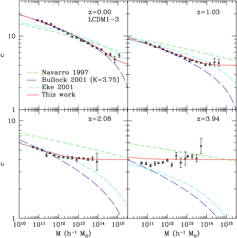
Figure 15.— Predicted and simulated median concentration as a function of halo mass for simulations LCDM1–3. Black symbols are results measured in simulations and error bars the standard deviation among halos of the same mass divided by the square root of the halo number in the bin, and these data are in excellent agreement with those presented in Figure 2 of Zhao et al. (2003b). Solid red lines are our model predictions, while short-dashed green, long-dashed dark blue, and dot-dashed blue lines are predictions of the NFW model, the B01 model, and the E01 model, respectively. The B01 model has several versions of model parameters and here we adopt the version with $F=0.01$ and $K=3.75$.

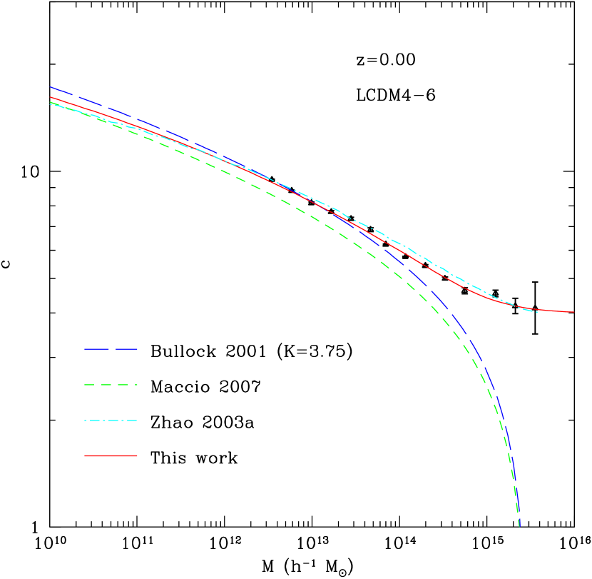
Figure 16.— Predicted and simulated median concentration as a function of halo mass for simulations LCDM4–6. Symbols and error bars are the same as in Figure 15. Solid red lines are our model predictions, while short-dashed green, long-dashed dark blue, and dot-dashed blue lines are predictions of the model of Macció et al. (2007), the B01 model, and the Z03a model, respectively.

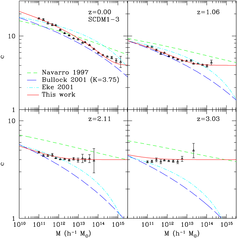
Figure 17.— Predicted and simulated median concentration as a function of halo mass for simulations SCDM1–3. Symbols and lines are the same as in Figure 15.

Z03a found that the scale radius $R_{s}$ is tightly correlated with the mass $M_{s}$ enclosed by it. With this tight correlation, one can predict halo concentration from the MAHs. Using the MAH model given in last section, we can predict the halo concentration according to the Z03a model. The prediction of this model is shown in Figure 16 as the dot-dashed line. For comparison, we also show predictions of the B01 model and the model of Macció et al. (2007) in the same figure. As one can see, the prediction of the Z03a model is more accurate than the other two models, particularly for high mass halos.

Although the model of Z03a matches well the simulation data, it is not easy to implement. Here we use our simulation results to find a new model that is more accurate and easier to implement. Let us first consider an SF case with a given linear power index. In this case, the halos of a given mass have a uniquely determined time $t_{F}$ when their main progenitors reach a fixed fraction $F$, e.g., $50\%$, of their final mass. There is thus a one-to-one correspondence between the MAH and $t_{F}$. If the concentration of a halo is fully determined by its MAH, one may build a model to link $t_{F}$ and the final halo concentration. In principle, such a relation can be found for $t_{F}$ at an arbitrarily fixed fraction of the final halo mass, but the resulting relation may be very different for scale-free models of different power indices. What we are seeking is a value of $F$ with which the relations between $c$ and $t_{F}$ are the same for all the scale-free models.

After many trials, we find that the concentration of a halo is tightly correlated with the time $t_{0.04}$ when its main progenitor gained $4\%$ of its final mass. This relation is almost identical for $n=0,\,-1$ and $-2$, as shown in Figure 18, but is slightly lower for the $n=1$ model. Since for realistic cosmological models, the effective slope of the linear power spectrum on scales of halos that can form is always less than 0, we exclude the result of the $n=1$ model in modeling the $c$–$t_{0.04}$ relation. We find that the relation given by the other three models can be accurately described by the following simple expression:

$$c=\left[4^{8}+(t/t_{\rm 0.04})^{8.4}\right]^{1/8}=4\times\left[1+(t/3.75t_{\rm 0.04})^{8.4}\right]^{1/8}\,.$$ (13)

Nontrivially, this same relation also applies very well to the CDM models, as shown in the small window of Figure 18.

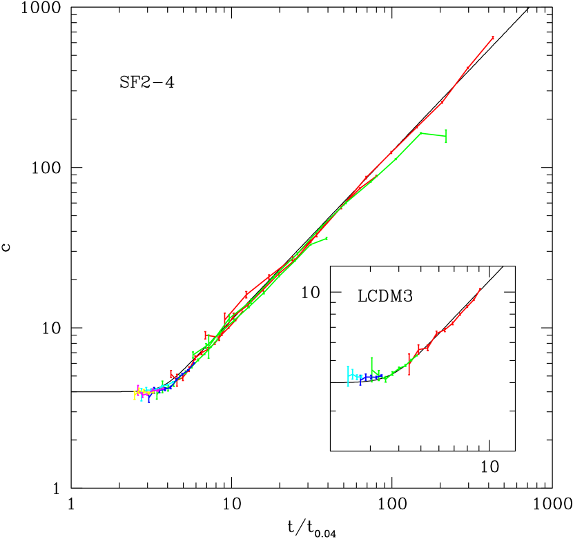
Figure 18.— Concentration of the final offspring halo as a function of the universe age when its main progenitor first gained $4\%$ of the final halo mass. Results are shown for scale-free cases with $n=0,\,-1,\,-2$ and for LCDM3. Different colors represent different snapshots, and the red line is for $z=0$. The solid curves are given by Equation (13).

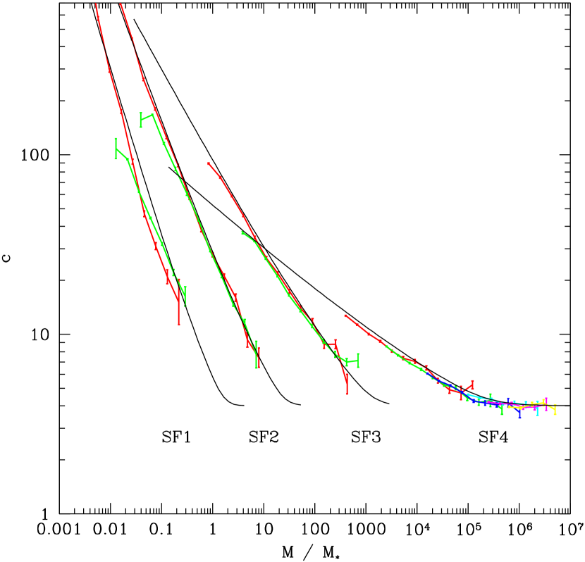
Figure 19.— Halo median concentration as a function of halo mass for scale-free models with $n=1,\,0,\,-1,$ and $-2$. Colored symbols are results measured in simulations and error bars are the standard deviation among halos of the same mass divided by the square root of the halo number in the bin. Smooth lines are our model predictions. For clarity, both the simulation data and the model predictions have been shifted in horizontal direction by -1, 0, 1.5, and 3.5 for SF1, SF2, SF3, and SF4, respectively.

From our MAH model described in Section 3, we can easily compute the time $t_{0.04}$ for a halo of mass $M$. We can then predict its concentration straightforwardly by using Equation (13). The concentration–halo mass relations so obtained are shown as the solid lines in Figure 19 for the SF models, and in Figures 15–17 for the CDM models. Comparing the model predictions with the corresponding simulation data, we see that our model works accurately for all the models and for halos at different redshifts. The typical error of our prediction is less than 5%. Somewhat larger deviations ($\sim 10\%$) seen for halos of mass $\sim 10^{11}\,{\rm M_{\odot}}$ at redshift $z\sim 3$ could be a result of numerical inaccuracy in the simulations, because these halos are not well relaxed. Compared with early models, ours is clearly a very significant improvement. In Appendix B, we describe step-by-step how to use Equation 13 to predict the concentration–mass relation at any given redshift for a given cosmological model.

It should be pointed out that both our model and the model of NFW are based on the correlation between halo concentration and a characteristic formation time. However, the two models have several important differences. First, in the NFW model the formation time was defined as the epoch when half of the halo mass $M$ has been assembled in its progenitors of masses exceeding $0.01M$, while in our model the time is defined as the epoch when its main progenitor has gained $4\%$ of the halo mass. Second, the ways to relate the concentration to the characteristic time are also different. NFW assumed that the inner density at $R_{s}$ of a halo is proportional to the mean density of the universe at the formation time, while we relate the halo concentration and the characteristic time by Equation (13). Finally, NFW used the extended Press–Schechter formula to compute the formation time, while we use our model of MAHs to calculate the time $t_{0.04}$. These differences make a very big difference in the model predictions, as shown above.

4.2. The Evolution of Halo Structure Along the Main Branch

The model described above can also be used to predict how halo structural properties, such as $c$, $R_{s}$, $\rho_{s}$, $M_{s}$, and $V_{s}$, and hence density profile evolve along the main branch. For a given MAH, $M(z)$, we can estimate $t_{0.04}$ for the current halo, $M(z)$ [corresponding to the virial radius $R(z)$ and the circular velocity $V(z)$], at the redshift $z$ in question, and use the model described above to obtain $c$ at $z$. Since the virial radius $R$ is determined by $M(z)$, we can then obtain $R_{s}$, $\rho_{s}$, $M_{s}$, and $V_{s}$ through $R_{s}=R/c$, Equations (4) and (5), respectively. The solid lines in Figure 20 show the model predictions in comparison with the simulation results of LCDM1–3 shown by circles connected by lines. Clearly, our model also works very well in describing these evolutions. These results demonstrate that, for a given halo, our model cannot only predict how its total mass grows with time, but can also predict how its inner structure changes with time. Thus, one can plot its NFW density profile at any point of the main branch, and can obtain the density evolution in spherical shell of any radius.

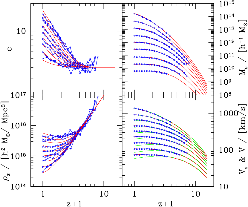
Figure 20.— Predicted (smooth lines) and simulated (symbols connected with lines) evolution of the median $c$, $\rho_{s}$, $M_{s}$, and $V_{s}$ for halos of nine different final masses in simulations LCDM1–3. The increasing direction of final halo mass among different lines in left/right panels is downward/upward. Here simulated $\rho_{s}$, $M_{s}$, and $V_{s}$ are estimated with the simulated median $c$ and the predicted halo mass. For comparison, evolution of circular velocity at the virial radius, $V$, is also plotted in the lower right panel as dashed lines.

As one can see, for low-mass halos, $\rho_{s}$, $M_{s}$, $V_{s}$, hence also $R_{s}$, all remain more or less constant at low redshift, suggesting that the inner structures of these halos change only little in the late stages of their evolution. Since by definition the virial radius $R$ increases with time, the concentration of such halos increases rapidly with decreasing redshift. Note that the circular velocity at the virial radius actually decreases with time for such halos at late time, as shown by the dashed lines in the lower-right panel of Figure 20. On the other hand, for massive halos, $\rho_{s}$, $M_{s}$, $V_{s}$, and $R_{s}$ all change rapidly with redshift even at $z\sim 0$, implying that the inner structures of these halos are still being adjusted by the mass accretion. Therefore, the concentration of such halos increases very slowly or even remains constant with redshift, much different from the W02 model which argues that $c\propto a$. All these behaviors had been illustrated clearly in Z03a and Z03b. As discussed in Z03a, these different behaviors are mainly due to the fact that massive halos are still in their early growth phases, which is characterized by rapid halo growth dominated by major mergers, effectively reconfiguring and deepening the gravitational potential wells and causing the collisionless dark matter particles to undergo dynamical relaxation and to mix up sufficiently to form the core structure, while low-mass halos have reached the late growth phase, which is characterized by slower quiescent growth predominantly through accretion of material onto the halo outskirt, little affecting the inner structure and potential.

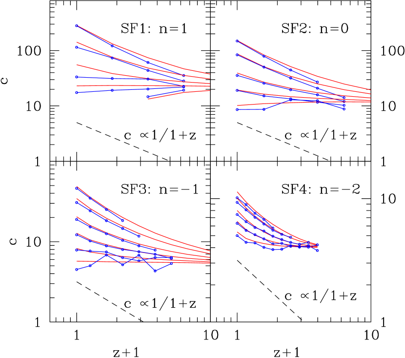
Figure 21.— Predicted (smooth lines) and simulated (symbols connected with lines) evolution of the median $c$ for halos of different final masses in simulations SF1–4. The increasing direction of final halo mass among different lines is from top to bottom. For comparison, assumption of W02, $c\propto 1/(1+z)$, is also plotted in each panel as the dashed line.

Figure 21 presents the model predictions of the evolution of median $c$ in comparison with the simulation results of SF1–4. It is very interesting that the simulated median concentrations of massive halos in each SF model also remain constant but the values are not $4$ except for SF4 ($n=-2$). This is not surprising: as shown in Figure 10, the mass accretion of SF4 halos, which is the fastest in these SF models, is very similar to the CDM cases and thus triggers dynamical relaxation and core-structure formation, resulting a constant concentration of about 4; while for the rest SF models, mass accretion is more or less slower and even the massive straight-line-MAH halos is in their slow growth regime ($t/t_{0.04}>3.75$; see Figure 18) and, according to Equation (13), progenitors on these straight line MAHs, which have time-invariant $t/t_{0.04}$, will all have constant but $n$-dependant concentrations. According to Section 3.1, all median MAHs in SF cases asymptote $M\propto(1+z)^{-6/(3+n)}$ and, in an Einstein de Sitter universe, universe age $t\propto(1+z)^{-1.5}$. Combining these two relations with Equation (13), we find halo median concentrations also have a unique asymptotic behavior at high redshift: $c\cong 29.37,\,12.61,\,5.477$, and $4.007$ for $n=1,\,0,\,-1$, and $-2$, respectively. These numbers are well verified in Figure 21 (except that in the SF1 case $c$ should be shifted a little bit when compared with the simulation results because a short-wavelength cutoff in the linear power spectrum have been included in this simulation) and, for comparison, assumption of W02, $c\propto 1/(1+z)$, is also plotted in each panel of the figure. Actually, for this kind of self-similar straight-line MAHs, any concentration model which claim that halo concentration is tightly correlated to its MAH should predict a constant concentration, as required by logic. For the most massive and so very rare halos which grow faster and faster, as demonstrated in the two upper panels of Figure 10, our model predict a decrease of concentration with time, as its $t/t_{0.04}$ is diminishing. This very interesting behavior is again supported by the simulation results and worth further detailed study.

4.3. Comparison with the Zhao et al. (2003a) Model

As mentioned above, the Z03a model for the halo concentrations is based on the tight correlation between $R_{s}$ and $M_{s}$. In Figure 22 we show the $M_{s}$–$R_{s}$ relation obtained from the simulations used in this paper. Clearly, for a given mass, $M_{s}$ and $R_{s}$ are tightly correlated, and the relation is well described by $M_{s}\propto R_{s}^{3\alpha}$ with $\alpha\simeq 0.55$. The value of $\alpha$ is between the values $0.48$ and $0.64$ obtained in Z03a for the late slow and early fast growth regimes, respectively. This suggests that the model we are proposing here is closely related to that of Z03a. To show this more clearly, let us start with Equation (10) in Z03a:

$${[\ln(1+c)-c/(1+c)]c^{-3\alpha}\over[\ln(1+c_{0})-c_{0}/(1+c_{0})]c_{0}^{-3\alpha}}=\left[{\rho(z)\over\rho_{0}}\right]^{\alpha}\left[{M(z)\over M_{0}}\right]^{1-\alpha}\,.$$ (14)

The function of $c$ in square brackets on the left side behaves like a power law for moderate concentrations and then we will use a power law function instead. Suppose that we have a halo whose main branch reaches $4\%$ of its current mass at a time $t_{0.04}$ and assume that the concentration of the progenitor at $t=t_{0.04}$ is 4. Substituting quantities of subscript 0 in the above equation with quantities at $t=t_{0.04}$ gives

$${\left(\frac{c}{4}\right)^{\beta-3\alpha}}=\left({\rho\over\rho_{0.04}}\right)^{\alpha}25^{(1-\alpha)}\,,$$ (15)

where $\beta\simeq 0.603$ for moderate $c\leq 25$. We can then obtain

$$c=4\left[\left({\rho\over\rho_{0.04}}\right)^{\alpha}25^{1-\alpha}\right]^{1/(\beta-3\alpha)}=4\left[\frac{1}{4}\left({\rho\over\rho_{0.04}}\right)^{-1.05/2}\right]\,$$ (16)

assuming $\alpha=0.55$. This is very similar to relation (13) at $t>3.75t_{0.04}$, indicating that the model proposed here is consistent with that of Z03a. Indeed, for a given MAH, the redshift when $t=3.75\times t_{0.04}$ is uniquely determined. We found that this redshift separates well the fast growth regime ($t<3.75t_{0.04}$) from the slow growth regime ($t>3.75t_{0.04}$). In the fast growth regime all halos have about the same median concentration $c\sim 4$ independent of halo mass, while in the slow growth regime the concentration scales with time as $\sim 4(t/3.75t_{0.04})^{1.05}$. This is exactly the proposal made in Z03a, Z03b that concentration evolution of a halo depends much on its mass accretion rate and the faster the mass grows, the slower the concentration increases.

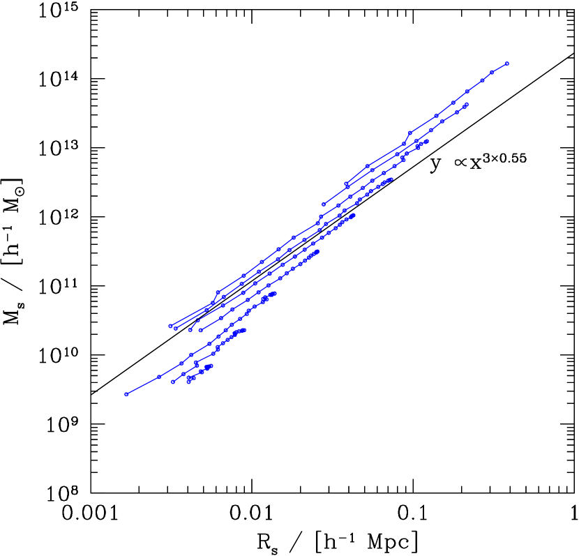
Figure 22.— Inner mass $M_{s}$ vs. inner radius $R_{s}$ along the simulated median MAH obtained from LCDM1–3. Results are shown for halos with nine different final masses, the same as those shown in Figure 20.

5. Conclusions and Discussion

A large amount of observations have constrained cosmological parameters and the initial density fluctuation spectrum to a very high accuracy. However, cosmological parameters change with time and the power index of the power spectrum varies with mass scale dramatically in the so-called concordance $\Lambda$CDM cosmology. Thus, any successful model for its structural evolution should work well simultaneously for various cosmological models and different power spectra.

In this paper, we use a large set of $N$-body simulations of various structure formation models to study the MAHs, the mass and redshift dependence of concentrations and the concentration evolution histories of dark matter halos. We find that our simulation results cannot be described by the much-used empirical models in the literature. Using our simulation results, we developed new empirical models for both the MAHs and the concentration evolution histories of dark matter halos, and the latter can also be used to predict the mass and redshift dependence of halo concentrations. These models are universal, in the sense that the same set of model parameters works well for different cosmological models and for halos of different masses at different redshifts. Our model predictions also match the PINOCCHIO MAHs very well, which are automatically output by the Lagrangian semianalytic code PINOCCHIO without any postprocessing and so are much independent of our numerical simulations and of our definitions of halo merger trees. These models are also simple and easy to implement, making them very useful in modeling the growth and structure of the dark matter halo population.

We found that, in describing the median MAH of dark matter halos, some degree of universality can be achieved by using $\delta_{c}(z)$, the critical overdensity for spherical collapse, to represent the time, and $\sigma(M)$, the rms of the linear density field on mass scale $M$, to represent the mass. This is consistent with the Press–Schechter (PS) theory, in which the dependence on cosmology and power spectrum is all through $\delta_{c}(z)$ and $\sigma(M)$. A more universal relation can be found by taking into account the local slope of the power spectrum on the mass scale in consideration. This is again expected, because the growth of an average halo in a given cosmological background is determined by the perturbation power spectrum on larger scales. Indeed, in the extended PS theory, the average mass accretion rate of a halo of a given mass depends both on $\sigma(M)$ and its derivative. However, the exact dependence on the shape of the power spectrum in our empirical model is actually different from that given by the extended PS theory, as demonstrated clearly by the discrepancy between our results and the model of van den Bosch (2002), which is based on the extended PS theory (see Figures 10–12). We find that another modification is required in order to correct the deviation of halos corresponding to relatively low peaks. We suggest that such deviation is due to the neglect of the large-scale tidal field on the formation of dark matter halos, as found in Wang et al. (2007). Thus, the empirical model we find for the halo accretion histories may help us to develop new models for the mass function and merger trees of dark matter halos. In addition, we find that a linear relation between $s(M)$ [defined in Equation (8)] and $\delta_{c}(z)$ is also a good approximation for individual halos, although the slope may change from halo to halo. Thus, the MAHs of individual halos may be modeled with a set of straight lines, in the $s(M)$–$\delta_{c}(z)$ space, with different slopes specified by a distribution function. Research along these lines is clearly worthwhile, and we plan to come back to these problems in forthcoming papers.

Our other finding is that the concentration of a halo is strongly correlated with $t_{0.04}$, the age of the universe when its progenitor on the main branch first reaches $4\%$ of its current mass. This is consistent with the general idea that the structure of a dark matter halo is correlated with its formation history. The concentration of a halo selected at a given redshift is determined by the ratio of the universe age at this redshift, $t$, to $t_{0.04}$. If this ratio is smaller than 3.75, the halo is in the fast growth regime and its concentration is expected to be $c\sim 4$, independent of its mass. For a halo in the fast growth regime, its first $4\%$ mass settled down at a late epoch (of age $>t/3.75$) and so has low density. In addition, its current accretion rate is large in the sense that it only takes a time interval of much less than $2.75t/3.75$ to gain the 96 percent of mass remaining. Such accretion is expected to have a significant impact on the inner structure that is not very dense, and so the inner structure of this halo is adjusted constantly by the mass accretion. In contrast, for a halo in the slow growth regime ($t/t_{0.04}>3.75$), its first $4\%$ mass settled down at an early epoch when the universe age was smaller than $t/3.75$, and so this fraction of the mass is expected to settle into a very dense clump. Also, for such a halo, the current accretion rate is small in the sense that it takes a time interval of more than $2.75t/3.75$ to gain the $96\%$ of mass remaining. Such slow accretion is not expected to have a significant impact on the inner dense structure that has already formed. All these are in qualitative good agreement with the results presented in Z03a. Our model can also be used to predict accurately how halo structural properties, such as $c$, $R_{s}$, $\rho_{s}$, $M_{s}$ and $V_{s}$, and hence its density profile evolve along the main branch, making it very useful for our understanding of the formation and evolution of dark matter halos. Assuming that the NFW profile is a good approximation for the halo density profile, the model can predict too the MAHs, the mass and redshift dependence of concentrations and the concentration evolution histories for different halo definitions. In a forthcoming paper, we will apply this model to individual halos.

We found that in a self-similar cosmology halos on some characteristic mass scale have a straight-line median MAH and a time-invariant median concentration. All halos asymptote these median features at high redshift: halos under this mass scale will grow slower and slower on average and their concentration will increase with time; while halos above this mass scale will grow faster and faster on average and their concentration will decrease. On the other hand, in $\Lambda$CDM and OCDM cases, both the decrease of cosmological density parameter $\Omega_{m}$ with time and the increase of power index of the power spectrum with mass scale will slow down the halo mass growth rate, inducing that at the present time halos on nearly all mass scales show two distinct phases in their mass growth histories, as found by Z03b and Z03a. Z03a and Z03b also pointed out that when halo mass accretion rate reaches some criteria, the fast mass growth will trigger dynamical relaxation and core-structure formation, resulting in a constant concentration of about 4. Here we found another mechanism that will lead to a time-invariant concentration along the main branch of a halo merger tree: a self-similar straight-line MAH will induce a constant concentration, as required by logic, and when the mass accretion rate is below the above criteria, the value of this constant is determined by the accretion rate and is always larger than 4.

In the appendices A and B, we give a detailed user’s guide on how to use the results of the present paper to compute the median mass accretion history and the concentration of dark matter halos for a given cosmological model.

Appendix A Calculating the median mass accretion history of halos

For a given cosmological model, one can calculate $\delta_{c}(z)=\delta^{\prime}_{c}[\Omega_{m}(z),\Omega_{\Lambda}(z)]/D(z)$ for a given redshift $z$, where $\delta^{\prime}_{c}[\Omega_{m}(z),\Omega_{\Lambda}(z)]$ is the conventional spherical collapse threshold at redshift $z$, $D(z)$ is the linear growth factor normalized to 1 at redshift $z=0$, and $\delta_{c}(z)$ is the collapse threshold for the density field linearly evolved to $z=0$. Given a linear power spectrum at $z=0$, one can also calculate the rms density fluctuation $\sigma(m)$ for a spherical volume of mass $m$, as well as $s(m)$. Once these quantities are obtained, one can calculate the median mass growth history of dark matter halos of mass $M_{\rm obs}$ at redshift $z_{\rm obs}$, i.e., the median mass $M(z|z_{\rm obs},M_{\rm obs})$ of their main progenitors at a higher redshift $z>z_{\rm obs}$. The step-by-step procedure is as follows.

1. With $\sigma(M_{\rm obs})$, $s(M_{\rm obs})$ and $\delta_{c}(z_{\rm obs})$ for halos of mass $M_{\rm obs}$ at redshift $z_{\rm obs}$, one can calculate $w(z_{\rm obs},M_{\rm obs})$ according to Equation (7) and the shift $p(z_{\rm obs},z_{\rm obs},M_{\rm obs})$ according to Equation (11). Let $z=z_{\rm obs}$ and $M=M_{\rm obs}$ temporarily.

2. One can obtain the accretion rate $d\lg\sigma(M)/{d\lg\delta_{c}(z)}$ at this redshift by substituting the above $w$ and $p$ into Equation (12).

3. At an incrementally higher redshift $z^{\prime}=z+\Delta z$, one can calculate the new critical collapse threshold $\delta_{c}(z^{\prime})$ at $z^{\prime}$, and its change $\Delta\lg\delta_{c}(z)$ between $z^{\prime}$ and $z$, and hence obtain the change in $\lg\sigma(M)$ through $\Delta\lg\sigma(M)=d\lg\sigma(M)/{d\lg\delta_{c}(z)}\times\Delta\lg\delta_{c}(z)$. One can then get a new $\sigma(M^{\prime})$, with $M^{\prime}$ being the median mass of the main progenitors at $z^{\prime}$. The mass $M^{\prime}$ can be obtained from $\sigma$ through the function $\sigma(m)$.

4. In order to trace the history further backward, one needs to calculate $w(z^{\prime},M^{\prime})$ according to Equation (7) and calculate the shift $p(z^{\prime},z_{\rm obs},M_{\rm obs})$ according to Equation (3.2). Let $z=z^{\prime}$, $M=M^{\prime}$, and repeat steps 2 and 3.

Then step by step, one can trace the MAH backwards to high redshift. One can also calculate the halo radius $R(z)$ and halo circular velocity $V(z)$ along this MAH according to Equations (2 and 3) by setting $\Delta_{h}=\Delta_{\rm vir}$ as defined in Section 1.

Appendix B Calculating the halo concentration

For a given MAH ending at $[z_{\rm obs},M_{\rm obs}]$ in a given cosmology, one can predict concentrations for all the main progenitors at different redshifts in addition to the final offspring, i.e., one can obtain the concentrations along the MAH, $c(z|z_{\rm obs},M_{\rm obs})$. Then many other useful quantities can be calculated as shown below. There are two steps in computing the concentrations.

1. From a given MAH, $M(z|z_{\rm obs},M_{\rm obs})$, one can compute $z_{0.04}$, the redshift at which the main progenitor of the main progenitor halo at $z(\geq z_{\rm obs})$ grows to $0.04M$, where $M$ is the mass of the main progenitor halo at $z$.

2. In the given cosmology, one can calculate the ages of the universe, $t$ and $t_{0.04}$, at these two redshifts, $z$ and $z_{0.04}$, and obtain $c(z|z_{\rm obs},M_{\rm obs})$ by substituting them into Equation (13).

3. Furthermore, one can calculate the characteristic inner quantities of the halo along the MAH, such as $R_{s}(z|z_{\rm obs},M_{\rm obs})$, $\rho_{s}(z|z_{\rm obs},M_{\rm obs})$, $M_{s}(z|z_{\rm obs},M_{\rm obs})$ and $V_{s}(z|z_{\rm obs},M_{\rm obs})$, according to the definition of $c$ and Equations (2–5), and hence can plot the NFW density profile at any point of the MAH according to Equation (1).

In the literature, there are several definitions for halo radius. Assuming that the NFW profile is a good approximation for the halo density profile, one can predict the MAHs and the concentration evolution histories for different halo definitions, because halos of different definitions have the same inner structures (such as $R_{s}$, $\rho_{s}$ and $M_{s}$) although their boundaries are different. For example, according to Equations (4 and 5), one can calculate $c_{\rm 200c}(z|z_{\rm obs},M_{\rm obs})$, $M_{\rm 200c}(z|z_{\rm obs},M_{\rm obs})$ , $V_{\rm 200c}(z|z_{\rm obs},M_{\rm obs})$ for halo definition $\Delta_{h}(z)=200/\Omega_{m}(z)$ and one can also calculate $c_{\rm 200m}(z|z_{\rm obs},M_{\rm obs})$, $M_{\rm 200m}(z|z_{\rm obs},M_{\rm obs})$, $V_{\rm 200m}(z|z_{\rm obs},M_{\rm obs})$ for halo definition $\Delta_{h}(z)=200$.

Note that $c(z|z_{\rm obs},M_{\rm obs})$ obtained with steps 1 and 2 is the concentration of a main progenitor of a halo of mass $M_{\rm obs}$ at $z_{\rm obs}$. As we pointed out in Section 3.2, this population of main progenitors of mass $M$ at $z$ is not statistically the same as the whole population of halos of mass $M$ at $z$, although in some cases the difference between them is negligible. The former population resides in environment of more frequent mergers and so has slightly smaller concentration. In any case, one can easily compute $c(M,z)$ for the whole population of halos of mass $M$ at $z$ if one sets $z_{\rm obs}=z$ and $M_{\rm obs}=M$ in the above calculation.

Appendix C A calculator, a user-friendly code and tables available on internet

A calculator which allows one to interactively generate the median MAHs, the concentration evolution histories and the mass and redshift dependence of concentrations of dark matter halos is provided at http://www.shao.ac.cn/dhzhao/mandc.html, together with a user-friendly code to make the relevant calculations. The calculator and the code can be used for almost all current cosmological models with or without inclusion of the effects of baryons in the initial power spectrum. We also provide tables for median concentrations of halos with different masses at different redshifts in several popular cosmological models. Detailed instructions on how to use the calculator, the code and the tables can be found at the Web site.

References

- Bardeen et al. (1986) Bardeen, J. M., Bond, J. R., Kaiser N., & Scalay A. 1986, ApJ, 304, 15
- Bryan & Norman (1998) Bryan, G. L., & Norman, M., 1998, ApJ, 495, 80
- Bullock et al. (2001) Bullock, J. S., Kolatt, T. S., Sigad, Y., Somerville, R. S., Kravtsov, A. V., Klypin, A. A., Primack, J. R., & Dekel, A. 2001, MNRAS, 321, 559
- Eisenstein & Hu (1998) Eisenstein, D. J., & Hu, W. 1998, ApJ, 496, 605
- Eke, Navarro & Steinmetz (2001) Eke, V. R., Navarro, J.F., & Steinmetz, M. 2001, ApJ, 554, 114
- Gao et al. (2008) Gao, L., Navarro, J. F., Cole, S., Frenk, C. S., White, S. D. M., Springel, V., Jenkins, A., & Neto, A. F. 2008, MNRAS, 387, 536
- Hockney & Eastwood (1981) Hockney, R. W., & Eastwood, J. W. 1981, Computer Simulation Using Particles (McGraw Hill, New York)
- Hoffman et al. (2007) Hoffman, Y., Romano-Díaz, E., Shlosman, I., & Heller, C. 2007, ApJ, 671, 1108
- Jenkins et al. (2001) Jenkins, A., Frenk, C. S., White, S. D. M., Colberg, J. M., Cole, S., Evrard, A. E., Couchman, H.M. P., & Yoshida, N. 2001, MNRAS, 321, 372
- Jing (2000) Jing, Y. P. 2000, ApJ, 535, 30
- Jing & Suto (1998) Jing, Y. P., & Suto Y. 1998, ApJ, 494, L5
- Jing & Suto (2002) Jing, Y. P., & Suto Y. 2002, ApJ, 574, 538
- Jing, Suto & Mo (2007) Jing, Y. P., Suto, Y., & Mo, H. J. 2007, ApJ, 657, 664
- Kitayama & Suto (1996) Kitayama, T., & Suto, Y. 1996, MNRAS, 280, 638
- Lacey & Cole (1994) Lacey, C., & Cole, S. 1994, MNRAS, 271, 676
- Li et al. (2007) Li, Y., Mo, H. J., van den Bosch, F. C., & Lin, W. P. 2007, MNRAS, 379, 689
- Lu et al. (2006) Lu, Y., Mo, H. J., Katz, N., & Weinberg, M. D. 2006, MNRAS, 368, 1931
- Macció et al. (2007) Macció, A. V., Dutton, A. A., van den Bosch, F. C., Moore, B., Potter D., & Stadel J. 2007, MNRAS, 378, 55
- Macció et al. (2008) Macció, A. V., Dutton, A. A., & van den Bosch, F. C. 2008, MNRAS, 391, 1940
- McBride et al. (2009) McBride, J., Fakhouri, O., & Ma, C. P. 2009, MNRAS, 398, 1858
- Miller et al. (2006) Miller, L., Percival., W. J., Croom, S. M., & Babić, A. 2006, A&A, 459, 43
- Monaco et al. (2002) Monaco, P., Theuns, T., Taffoni, G., Governato, F., Quinn, T., & Stadel, J. 2002, ApJ, 564, 8
- Navarro, Frenk, & White (1997) Navarro, J. F., Frenk, C. S., & White, S. D. M. 1997, ApJ, 490, 493
- Neistein et al. (2008) Neistein, E., & Dekel, A. 2008, MNRAS, 383, 615
- Neistein et al. (2006) Neistein, E., van den Bosch, F. C., & Dekel, A. 2006, MNRAS, 372, 933
- Schmidt & Allen (2007) Schmidt, R. W., & Allen, S. W. 2007, MNRAS, 379, 209
- van den Bosch (2002) van den Bosch, F. C. 2002 MNRAS, 331, 98
- Wang et al. (2007) Wang, H. Y., Mo, H. J., & Jing, Y. P. 2007, MNRAS, 375, 633
- Wechsler et al. (2002) Wechsler, R. H., Bullock, J. S., Primack, J. R., Kravtsov, A. V., & Dekel, A. 2002, ApJ, 568, 52
- Zhao et al. (2003a) Zhao, D. H., Mo, H. J., Jing, Y. P., & Boerner, G. 2003a, MNRAS, 339, 12
- Zhao et al. (2003b) Zhao, D. H., Jing, Y. P., Mo, H. J., & Boerner, G. 2003b, ApJ, 597, L9