Spectroscopic implications from the combined analysis of processes with pseudoscalar mesons

Abstract

In the analysis a status and parameters of the scalar, vector, and tensor mesonic resonances are obtained and compared with other results. Possible classification of the resonance states in terms of the SU(3) multiplets is discussed.

Outline:

• Motivation

• Method of analysis

• Analysis of the isoscalar-scalar sector

• Analysis of the isovector $P$-wave of $\pi\pi$ scattering

• Analysis of the isoscalar-tensor sector

• Spectroscopic implications from the analysis

I Motivation

The spectroscopy of light mesons plays an important role in understanding the strong interactions at low energies. Among possibilities to study the spectrum of light mesons, analysis of the $\pi\pi$ interaction is particularly useful and, therefore, it has always been an object of continuous theoretical and experimental investigation PDG08 . Here, we present results of the coupled-channel analysis of data on processes $\pi\pi\to\pi\pi,K\overline{K},\eta\eta,\eta\eta^{\prime}$ in the channels with $I^{G}J^{PC}=0^{+}0^{++}$ and $0^{+}2^{++}$ and on the $\pi\pi$ scattering in the channel with $1^{+}1^{--}$.

The scalar sector is problematic up to now especially as to an assignment of the discovered mesonic states to quark-model configurations in spite of a big amount of work devoted to these problems (see, e.g., Ref. Ani06 and references therein). An exceptional interest to this sector is supported by the fact that there, possibly indeed, we deal with a glueball $f_{0}(1500)$ (see, e.g., Ref. PDG08 ; Ams96 ).

Investigation of vector mesons is up-to-date subject due to their role in forming the electromagnetic structure of particles and because our knowledge about these mesons is still too incomplete (e.g., in the Particle Data Group tables PDG08 (PDG) the mass of $\rho(1450)$ is ranging from 1250 to 1582 MeV).

In the tensor sector, among the thirteen discussed resonances, the nine states ($f_{2}(1430)$, $f_{2}(1565)$, $f_{2}(1640)$, $f_{2}(1810)$, $f_{2}(1910)$, $f_{2}(2000)$, $f_{2}(2020)$, $f_{2}(2150)$, $f_{2}(2220)$) must be confirmed in various experiments and analyses. For example, in the analysis of $p\overline{p}\to\pi\pi,\eta\eta,\eta\eta^{\prime}$, five resonances – $f_{2}(1920)$, $f_{2}(2000)$, $f_{2}(2020)$, $f_{2}(2240)$ and $f_{2}(2300)$ – have been obtained, one of which, $f_{2}(2000)$, is a candidate for the glueball Ani05 .

In our analysis, we have used both a model-independent method KMS96 , based on the first principles (analyticity and unitarity) directly applied to analysis of experimental data, and the multichannel Breit–Wigner forms. The former approach permits us to introduce no theoretical prejudice to extracted parameters of resonances, however, it is limited with the possibility to use only three coupled channels. Therefore, in more general cases, one has to use, e.g., the Breit–Wigner approach. Considering the obtained disposition of resonance poles on the Riemann surface, obtained coupling constants with channels, and resonance masses we draw particular conclusions about nature of the investigated states.

II Method of analysis

In both methods of analysis, we parametrized the $S$-matrix elements $S_{\alpha\beta}$ where $\alpha,\beta=1,2,\cdots,n$ denote channels, using the Le Couteur-Newton relations LeCou . This relations express the $S$-matrix elements of all coupled processes in terms of the Jost matrix determinant $d(k_{1},\cdots,k_{n})$ that is a real analytic function with the only square-root branch-points at the channel momenta $k_{\alpha}=0$.

In the model-independent approach, the $S$-matrix is determined on the 4- and 8-sheeted Riemann surfaces for the 2- and 3-channel cases, respectively. The matrix elements $S_{\alpha\beta}$ have the right-hand cuts along the real axis of the $s$ complex plane ($s$ is the invariant total energy squared), starting at the coupled-channels thresholds $s_{i}$ ($i=1,2,3$), and the left-hand cuts related to the crossed channels. The Riemann-surface sheets are numbered according to the signs of analytic continuations of the channel momenta $k_{i}=\sqrt{s-s_{i}}/{2}~{}~{}~{}~{}(i=1,2,3)$, as shown in Table 1.

Table 1: Signs of channel momenta on the eight sheets of the Rieman surface in the 3-channel case.

sheet:	I	II	III	IV	V	VI	VII	VIII
Im $k_{1}$	$+$	$-$	$-$	$+$	$+$	$-$	$-$	$+$
Im $k_{2}$	$+$	$+$	$-$	$-$	$-$	$-$	$+$	$+$
Im $k_{3}$	$+$	$+$	$+$	$+$	$-$	$-$	$-$	$-$

The model-independent method which essentially utilizes an uniformizing variable can be used only for the 2-channel case and under some conditions for the 3-channel one. Only in these cases we obtain a simple symmetric (easily interpreted) picture of the resonance poles and zeros of the $S$-matrix on an uniformization plane. The important branch points, corresponding to the thresholds of the coupled channels and to the crossing ones, are taken into account in the uniformizing variable.

The resonance representations on the Riemann surfaces are obtained with the help of formulas from Ref. KMS96 , expressing analytic continuations of the $S$-matrix elements to unphysical sheets in terms of those on sheet I that have only the zeros of resonances (beyond the real axis), at least, around the physical region. Then, starting from the resonance zeros on sheet I, one can obtain an arrangement of poles and zeros of resonance on the whole Riemann surface.

In the 2-channel case, we obtain three types of resonances described by a pair of conjugate zeros on sheet I: (a) in $S_{11}$, (b) in $S_{22}$, (c) in each of $S_{11}$ and $S_{22}$.

In the 3-channel case, we obtain seven types of resonances corresponding to seven possible situations when there are resonance zeros on sheet I only in $S_{11}$ – (a);   $S_{22}$ – (b);   $S_{33}$ – (c);   $S_{11}$ and $S_{22}$ – (d);   $S_{22}$ and $S_{33}$ – (e);   $S_{11}$ and $S_{33}$ – (f); and   $S_{11}$, $S_{22}$, and $S_{33}$ – (g).
A resonance of every type is represented by a pair of complex-conjugate clusters (of poles and zeros on the Riemann surface). Note that whereas the cases (a), (b) and (c) can be simply related to the representation of resonances by the Breit-Wigner forms, the cases (d), (e), (f) and (g) are practically lost at that description. The cluster type is related to the nature of state. For example, if we consider the $\pi\pi$, $K\overline{K}$, and $\eta\eta$ channels, then a resonance which is coupled relatively more strongly to the $\pi\pi$ channel than to the $K\overline{K}$ and $\eta\eta$ ones is described by the cluster of type (a). If the resonance is coupled more strongly to the $K\overline{K}$ and $\eta\eta$ channels than to the $\pi\pi$ one, then it is represented by the cluster of type (e) (say, the state with the dominant $s{\bar{s}}$ component). The flavour singlet (e.g., glueball) must be represented by the cluster of type (g) (of type (c) in the 2-channel consideration) as a necessary condition for the ideal case, if this state lies above the thresholds of considered channels.

We can distinguish, in a model-independent way, a bound state of colourless particles (e.g., $K\overline{K}$ molecule) and a $q{\bar{q}}$ bound state. Just as in the 1-channel case, the existence of the particle bound-state means the presence of the pole on the real axis under the threshold on the physical sheet, so in the 2-channel case, the existence of the particle bound-state in channel 2 ($K\overline{K}$ molecule) that, however, can decay into channel 1 ($\pi\pi$ decay), would imply the presence of a pair of complex conjugate poles on sheet II under the second-channel threshold without the corresponding shifted pair of poles on sheet III.

In the 3-channel case, the bound-state in channel 3 ($\eta\eta$) that, however, can decay into channels 1 ($\pi\pi$ decay) and 2 ($K\overline{K}$ decay), is represented by the pair of complex conjugate poles on sheet II and by shifted poles on sheet III under the $\eta\eta$ threshold without the corresponding poles on sheets VI and VII. This test KMS96 ; MPe93 is a multichannel analogue of the known Castillejo–Dalitz–Dyson poles in the one-channel case. According to this test, earlier in Ref. KMS96 , the interpretation of the $f_{0}(980)$ state as the $K\overline{K}$ molecule has been rejected because this state is represented by the cluster of type (a) in the 2-channel analysis of processes $\pi\pi\to\pi\pi,K\overline{K}$ and, therefore, it does not satisfy the necessary condition to be the $K\overline{K}$ molecule.

III Analysis of the isoscalar-scalar sector

Considering the $S$-waves of processes $\pi\pi\to\pi\pi,K\overline{K},\eta\eta,\eta\eta^{\prime}$ in the model-independent method, we performed two variants of the 3-channel analysis:
variant I: the combined analysis of $\pi\pi\to\pi\pi,K\overline{K},\eta\eta\,$;
variant II: analysis of $\pi\pi\to\pi\pi,K\overline{K},\eta\eta^{\prime}$.
Influence of the $\eta\eta^{\prime}$-channel in variant I and the $\eta\eta$-channel in variant II are taken into account via the background. Here, the left-hand cuts are neglected in the Riemann-surface structure assuming that contributions on these cuts are also included in the background.

Under neglecting the $\pi\pi$-threshold branch point (however, unitarity on the $\pi\pi$-cut is taken into account), the uniformizing variable is

$$w=\frac{k_{2}+k_{3}}{\sqrt{m_{\eta}^{2}-m_{K}^{2}}}~{}~{}~{}~{}{\rm for~{}variant~{}I},$$ (1)

and

$$w^{\prime}=\frac{k_{2}^{\prime}+k_{3}^{\prime}}{\sqrt{\frac{1}{4}(m_{\eta}+m_{\eta^{\prime}})^{2}-m_{K}^{2}}}~{}~{}~{}~{}{\rm for~{}variant~{}II}.$$ (2)

The quantities related to variant II are primed.

On the $w$-plane, the Le Couteur-Newton relations are

$$S_{11}=\frac{d^{*}(-w^{*})}{d(w)},~{}~{}~{}~{}~{}~{}~{}~{}S_{22}=\frac{d(-w^{-1})}{d(w)},~{}~{}~{}~{}~{}~{}~{}~{}S_{33}=\frac{d(w^{-1})}{d(w)},$$ (3)

$$S_{11}S_{22}-S_{12}^{2}=\frac{d^{*}({w^{*}}^{-1})}{d(w)},~{}~{}~{}~{}~{}~{}~{}~{}S_{11}S_{33}-S_{13}^{2}=\frac{d^{*}(-{w^{*}}^{-1})}{d(w)}\,,$$ (4)

where the $d$-function is assumed in the form

$$d=d_{B}d_{res},$$ (5)

and the resonance part is

$$d_{res}(w)=w^{-\frac{M}{2}}\prod_{r=1}^{M}(w+w_{r}^{*})$$ (6)

with $M$ the number of resonance zeros. The background part is taken as

$$d_{B}=\mbox{exp}[-i\sum_{n=1}^{3}\frac{k_{n}}{m_{n}}(\alpha_{n}+i\beta_{n})],$$ (7)

where

$$\alpha_{n}=a_{n1}+a_{n\sigma}\frac{s-s_{\sigma}}{s_{\sigma}}\theta(s-s_{\sigma})+a_{nv}\frac{s-s_{v}}{s_{v}}\theta(s-s_{v}),$$ (8)

$$\beta_{n}=b_{n1}+b_{n\sigma}\frac{s-s_{\sigma}}{s_{\sigma}}\theta(s-s_{\sigma})+b_{nv}\frac{s-s_{v}}{s_{v}}\theta(s-s_{v})$$ (9)

with $s_{\sigma}$ the $\sigma\sigma$ threshold and $s_{v}$ a combined threshold of many opened channels in the vicinity of 1.5 GeV (e.g., $\eta\eta^{\prime},~{}\rho\rho,~{}\omega\omega$).

In variant II, the terms

$$a_{n\eta}^{\prime}\frac{s-4m_{\eta}^{2}}{4m_{\eta}^{2}}\theta(s-4m_{\eta}^{2})~{}~{}~{}~{}~{}{\rm and}~{}~{}~{}~{}~{}b_{n\eta}^{\prime}\frac{s-4m_{\eta}^{2}}{4m_{\eta}^{2}}\theta(s-4m_{\eta}^{2})$$ (10)

should be added to $\alpha^{\prime}_{n}$ and $\beta^{\prime}_{n}$ to account for an influence of the $\eta\eta$-channel.

As the data, we use the results of phase analyses given for phase shifts of the amplitudes $\delta_{ab}$ and for moduli of the $S$-matrix elements $\eta_{ab}=|S_{ab}|$ ($a,b=$1-$\pi\pi$, 2-$K\overline{K}$, 3-$\eta\eta$ or $\eta\eta^{\prime}$):

$$S_{aa}=\eta_{aa}e^{2i\delta_{aa}},~{}~{}~{}~{}~{}S_{ab}=\eta_{ab}e^{i\phi_{ab}}.$$ (11)

If below the $\eta\eta$-threshold there is the 2-channel unitarity, then the relations

$$\eta_{11}=\eta_{22},~{}~{}\eta_{12}=(1-{\eta_{11}}^{2})^{1/2},~{}~{}\phi_{12}=\delta_{11}+\delta_{22}$$ (12)

are fulfilled in this energy region.

The $\pi\pi$ scattering data, which range from the threshold up to 1.89 GeV, are taken from Ref. Hya73 ; expd1 . For $\pi\pi\to K\overline{K}$, practically all the accessible data are used expd2 . For $\pi\pi\to\eta\eta$, we used data for $|S_{13}|^{2}$ from the threshold to 1.72 GeV expd3 . For $\pi\pi\to\eta\eta^{\prime}$, the data for $|S_{13}|^{2}$ from the threshold to 1.813 GeV are taken from Ref. expd4 . We included all the five resonances discussed below 1.9 GeV.

In variant I, we got satisfactory description: for the $\pi\pi$ scattering, $\chi^{2}/\mbox{NDF}\approx 1.35$; for $\pi\pi\to K\overline{K}$, $\chi^{2}/\mbox{NDF}\approx 1.77$; for $\pi\pi\to\eta\eta$, $\chi^{2}/\mbox{N.exp.points}\approx 0.86$. The total $\chi^{2}/\mbox{NDF}$ is $345.603/(301-40)\approx 1.32$. From possible resonance representations by pole-clusters, the analysis selects the following one: the $f_{0}(600)$ is described by the cluster of type (a); $f_{0}(1370)$, type (c); $f_{0}(1500)$, type (g); $f_{0}(1710)$, type (b); and the $f_{0}(980)$ is represented only by the pole on sheet II and shifted pole on sheet III in both variants. The background parameters are: $a_{11}=0.2006$, $a_{1\sigma}=0.0146$, $a_{1v}=0$, $b_{11}=0$, $b_{1\sigma}=-0.01025$, $b_{1v}=0.0542$, $a_{21}=-0.6986$, $a_{2\sigma}=-1.4207$, $a_{2v}=-5.958$, $b_{21}=0.047$, $b_{2\sigma}=0$, $b_{2v}=6.888$, $b_{31}=0.6511$, $b_{3\sigma}=0.3404$, $b_{3v}=0$; $s_{\sigma}=1.638~{}{\rm GeV}^{2}$, $s_{v}=2.084~{}{\rm GeV}^{2}$.

In variant II, we got the following description: for the $\pi\pi$ scattering $\chi^{2}/\mbox{NDF}\approx 1.0$! for $\pi\pi\to K\overline{K}$ $\chi^{2}/\mbox{NDF}\approx 1.62$; for $\pi\pi\to\eta\eta^{\prime}$ $\chi^{2}/\mbox{N.exp.points}\approx 0.36$. The total $\chi^{2}/\mbox{NDF}$ is $282.682/(293-38)\approx 1.11$! In this case, the $f_{0}(600)$ is described by the cluster of type (a^′); $f_{0}(1370)$, type (b^′); $f_{0}(1500)$, type (d^′); and $f_{0}(1710)$, type (c^′). The background parameters are: $a_{11}^{\prime}=0.0111$, $a_{1\eta}^{\prime}=-0.058$, $a_{1\sigma}^{\prime}=0$, $a_{1v}^{\prime}=0.0954$, $b_{11}^{\prime}=b_{1\eta}^{\prime}=b_{1\sigma}^{\prime}=0$, $b_{1v}^{\prime}=0.047$, $a_{21}^{\prime}=-3.439$, $a_{2\eta}^{\prime}=-0.4851$, $a_{2\sigma}^{\prime}=1.7622$, $a_{2v}^{\prime}=-5.158$, $b_{21}^{\prime}=0$, $b_{2\eta}^{\prime}=-0.7524$, $b_{2\sigma}^{\prime}=2.6658$, $b_{2v}^{\prime}=1.836$, $b_{31}^{\prime}=0.5545$, $s_{\sigma}=1.638~{}{\rm GeV}^{2}$, $s_{v}=2.126~{}{\rm GeV}^{2}$.

Figure 1: The phase shift and module of the $S$-matrix element in the $S$-wave $\pi\pi$-scattering. The solid curve corresponds to variant I and the dashed curve to variant II.

Figure 2: The phase shift and module of the $S$-matrix element in $S$-wave of $\pi\pi\to K\overline{K}$. The solid curve corresponds to variant I and the dashed curve to variant II.

Figure 3: The squared modules of the $\pi\pi\to\eta\eta$ (upper figure) and $\pi\pi\to\eta\eta^{\prime}$ (lower figure) $S$-wave matrix elements.

In Figures 1-3, we show results of fitting to the experimental data and in Table 2 we indicate the obtained pole clusters for resonances on the eight sheets of the complex energy plane $\sqrt{s}$, on which the 3-channel $S$-matrix is determined ($\!\sqrt{s_{r}}={\rm E}_{r}-i\Gamma_{r}\!$).

Table 2: Pole clusters for the $f_{0}$-resonances in variants I and II.

Sheet		II	III	IV	V	VI	VII	VIII
variant I
$\!\!f_{0}(600)\!\!$	$\!\!{\rm E}_{r}\!\!$	598.2$\pm$13	585.8$\!\pm\!$14			505.8$\!\pm\!$16	518.2$\!\pm\!$15
	$\!\Gamma_{r}\!$	583$\!\pm\!$18	583$\!\pm\!$18			583$\!\pm\!$18	583$\!\pm\!$18
$\!f_{0}(980)\!$	$\!{\rm E}_{r}\!$	1013.1$\!\pm\!$4	983.6$\!\pm\!$9
	$\!\Gamma_{r}\!$	34.1$\!\pm\!$6	57.4$\!\pm\!$10
$\!f_{0}(1370)\!$	$\!{\rm E}_{r}\!$				1398.2$\!\pm\!$16	1398.2$\!\pm\!$18	1398.2$\!\pm\!$18	1398.2$\!\pm\!$13
	$\!\Gamma_{r}\!$				287.4$\!\pm\!$17	270.6$\!\pm\!$15	155$\!\pm\!$9	171.8$\!\pm\!$7
$\!f_{0}(1500)\!$	$\!{\rm E}_{r}\!$	1502.6$\!\pm\!$11	1479.5$\!\pm\!$13	1502.6$\!\pm\!$12	1496.7$\!\pm\!$12	1498$\!\pm\!$16	1496.8$\!\pm\!$12	1502.6$\!\pm\!$10
	$\!\Gamma_{r}\!$	357.1$\!\pm\!$15	139.4$\!\pm\!$12	238.7$\!\pm\!$13	139.9$\!\pm\!$14	191.2$\!\pm\!$17	87.36$\!\pm\!$11	356.5$\!\pm\!$14
$\!f_{0}(1710)\!$	$\!{\rm E}_{r}\!$		1708.2$\!\pm\!$12	1708.2$\!\pm\!$10	1708.2$\!\pm\!$13	1708.2$\!\pm\!$15
	$\!\Gamma_{r}\!$		142.3$\!\pm\!$9	160.3$\!\pm\!$8	323.3$\!\pm\!$14	305.3$\!\pm\!$13
variant II
$\!f_{0}(600)\!$	$\!{\rm E}_{r}\!$	616.5$\!\pm\!$8	621.8$\!\pm\!$10			598.3$\!\pm\!$11	593$\!\pm\!$12
	$\!\Gamma_{r}\!$	563$\!\pm\!$11	563$\!\pm\!$12			563$\!\pm\!$14	563$\!\pm\!$13
$\!f_{0}(980)\!$	$\!{\rm E}_{r}\!$	1009.3$\!\pm\!$3	986$\!\pm\!$6
	$\!\Gamma_{r}\!$	32$\!\pm\!$4	58$\!\pm\!$5.5
$\!f_{0}(1370)\!$	$\!{\rm E}_{r}\!$		1394.3$\!\pm\!$9	1394.3$\!\pm\!$11	1412.7$\!\pm\!$13	1412.7$\!\pm\!$14
	$\!\Gamma_{r}\!$		236.3$\!\pm\!$10	255.7$\!\pm\!$12	255.7$\!\pm\!$12	236.3$\!\pm\!$19
$\!f_{0}(1500)\!$	$\!{\rm E}_{r}\!$	1498.3$\!\pm\!$11	1502.4$\!\pm\!$9	1498.3$\!\pm\!$12	1498.3$\!\pm\!$13	1494.6$\!\pm\!$11	1498.3$\!\pm\!$14
	$\!\Gamma_{r}\!$	198.8$\!\pm\!$14	236.8$\!\pm\!$11	193$\!\pm\!$9	198.8$\!\pm\!$11	194$\!\pm\!$8	193$\!\pm\!$10
$\!f_{0}(1710)\!$	$\!{\rm E}_{r}\!$				1726.1$\!\pm\!$12	1726.1$\!\pm\!$13	1726.1$\!\pm\!$12	1726.1$\!\pm\!$10
	$\!\Gamma_{r}\!$				140.2$\!\pm\!$9	111.6$\!\pm\!$8	84.2$\!\pm\!$8	112.8$\!\pm\!$7

The $f_{0}(1370)$ and $f_{0}(1710)$ are represented by the pole clusters corresponding to states with the dominant $s\bar{s}$ component; $f_{0}(1500)$, with the dominant glueball component.

Note a surprising result obtained for the $f_{0}(980)$. This state lies slightly above the $K\overline{K}$ threshold and is described by the pole on sheet II and by the shifted pole on sheet III under the $\eta\eta$ threshold without the corresponding poles on sheets VI and VII, as it was expected for standard clusters. This corresponds to the description of the $\eta\eta$ bound state.

Masses and total widths of states should be calculated from the pole positions. If, when calculating these quantities, the resonance part of amplitude is taken in the form

$$T^{res}=\frac{\sqrt{s_{r}}\Gamma_{el}}{m_{res}^{2}-s_{r}-i\sqrt{s_{r}}\Gamma_{tot}},$$ (13)

we obtain values of masses and total widths of the $f_{0}$-resonances, presented in Table 3.

Table 3: Masses and total widths of the $f_{0}$-resonances (all in MeV).

	Variant I		Variant II
State	$m_{res}$	$\Gamma_{tot}$	$m_{res}$	$\Gamma_{tot}$
$f_{0}(600)$	835.3	1166	834.9	1126
$f_{0}(980)$	1013.7	68.2	1009.8	64
$f_{0}(1370)$	1408.7	343.6	1417.5	511
$f_{0}(1500)$	1544	714	1511.4	398
$f_{0}(1710)$	1715.7	321	1729.8	225.6

IV Analysis of the isovector $P$-wave of $\pi\pi$ scattering

In this sector we applied both the model-independent method and multichannel Breit–Wigner forms. We analyzed data in Ref. expd5 ; Hya73 , for the inelasticity parameter ($\eta$) and phase shift of the $\pi\pi$-scattering amplitude ($\delta$) ($S(\pi\pi\to\pi\pi)=\eta\exp(2i\delta)$), introducing three ($\rho(770)$, $\rho(1250)$ and $\rho(1550-1780)$), four (the indicated ones plus $\rho(1860-1910)$) and five (the indicated four plus $\rho(1450)$) resonances SB_NPA08 .

IV.1 The Model-Independent Analysis

Since in the data for the $P$-wave $\pi\pi$ scattering a deviation from elasticity is observed in the near-threshold region of the $\omega\pi$ channel, we considered explicitly the thresholds of the $\pi\pi$ and $\omega\pi$ channels and the left-hand one at $s=0$ in the uniformizing variable:

$$v=\frac{(m_{\omega}+m_{\pi^{0}})/2~{}\sqrt{s-4m_{\pi^{+}}^{2}}+m_{\pi^{+}}~{}\sqrt{s-(m_{\omega}+m_{\pi^{0}})^{2}}}{\sqrt{s\left[\left((m_{\omega}+m_{\pi^{0}})/2\right)^{2}-m_{\pi^{+}}^{2}\right]}}.$$ (14)

Influence of other channels which couple to the $\pi\pi$ one is supposed to be taken into account via the background.

On the $v$-plane, the resonance part of the 2-channel $S$-matrix element of $\pi\pi$-scattering $S_{res}$ has no cuts and has the form

$$S_{res}=\frac{d(-v^{-1})}{d(v)},$$ (15)

where $d(v)$ represents the contribution of resonances SB_NPA08 .

The background part is

$$S_{bg}=\exp\left[2i\left(\sqrt{\frac{s-4m_{\pi^{+}}^{2}}{s}}\right)^{3}\left(\alpha_{0}+\alpha_{1}~{}\frac{s-s_{1}}{s}~{}\theta(s-s_{1})+\right.\right.$$

$$\left.\left.\alpha_{2}~{}\frac{s-s_{2}}{s}~{}\theta(s-s_{2})\right)\right]\,,$$ (16)

where $\alpha_{i}=a_{i}+ib_{i}$, $s_{1}$ is the threshold of 4$\pi$ channel noticeable in the $\rho$-like meson decays and $s_{2}$ is the threshold of $\rho 2\pi$ channel. Due to allowing for the left-hand branch-point at $s=0$ in the $v$-variable, $a_{0}=b_{0}=0$. Furthermore, $b_{1}=0$ which is related to the experimental fact that the $P$-wave $\pi\pi$ scattering is elastic also above the 4$\pi$-channel threshold up to about the $\omega\pi^{0}$ threshold.

In Figure 4 we present results of fitting to the data with three, four and five resonances.

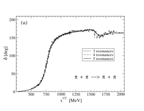
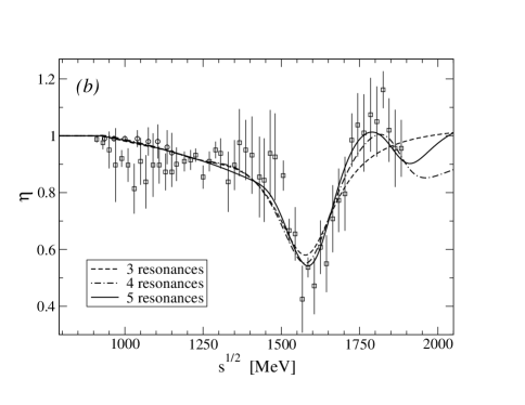
Figure 4: The phase shift of amplitude and module of the $S$-matrix element for the $P$-wave $\pi\pi$-scattering in the model-independent approach.

We obtained satisfactory description with the total $\chi^{2}/\mbox{NDF}$ equal to $~{}291.76/(183-15)=1.74$, $~{}278.50/(183-19)=1.70$, and $~{}266.14/(183-23)=1.66$ for the case of three, four and five resonances, respectively.

The $\rho(770)$ is described by the cluster of type (a) and the others by type (b). The background parameters are: $a_{1}=0.0093\pm 0.0199$, $a_{2}=0.0618\pm 0.0305$, and $b_{2}=-0.0135\pm 0.0371$ for the three-resonance, $a_{1}=0.0017\pm 0.2118$, $a_{2}=0.0433\pm 0.3552$, and $b_{2}=-0.0044\pm 0.4782$ for the four-resonance, and $a_{1}=0.0256\pm 0.0186$, $a_{2}=0.0922\pm 0.0335$, and $b_{2}=0.0011\pm 0.0478$ for the five-resonance descriptions. The positive sign of $b_{2}$ in the last case is more natural from the physical point of view.

Though the description can be considered, practically, as the same in all three cases, careful comparison of the obtained parameters and energy dependence of the fitted quantities suggests that the resonance $\rho(1900)$ is desired and that the $\rho(1450)$ might be also included improving slightly the description (at all events, its existence does not contradict to the data).

In Table 4, we show the pole clusters of the $\rho$-like states on the lower $\sqrt{s}$-half-plane (in MeV) (the conjugate poles on the upper half-plane are not shown).

Table 4: Pole clusters distributed on the sheets II, III, and IV for the case with five $\rho$-like resonances. $\sqrt{s_{r}}$ in MeV is given.

	II	III	IV
$\rho(770)$	$\!765.8\pm 0.6-i(73.3\pm 0.4)\!$	$\!778.2\pm 9.1-i(68.9\pm 3.9)\!$
$\rho(1250)$		$\!1251.4\pm 11.3-i(130.9\pm 9.1)\!$	$\!1251\pm 11.1-i(130.5\pm 9.2)\!$
$\rho(1470)$		$\!1469.4\pm 10.6-i(91\pm 12.9)\!$	$\!1465.4\pm 12.1-i(99.8\pm 15.6)\!$
$\rho(1600)$		$\!1634\pm 20.1-i(144.7\pm 23.8)\!$	$\!1592.9\pm 7.9-i(73.7\pm 11.7)\!$
$\rho(1900)$		$\!1882.8\pm 24.8-i(112.4\pm 25.2)\!$	$\!1893\pm 21.9-i(93.4\pm 19.9)\!$

Masses and total widths of the obtained $\rho$-states can be calculated from the pole positions on sheets II and IV for resonances of type (a) and (b), respectively. The obtained values are shown in Table 5.

Table 5: Calculated masses and total widths of the $\rho$-states (all in MeV).

	$m_{res}$	$\Gamma_{tot}$
$\rho(770)$	769.3$\pm$0.6	146.6$\pm$0.9
$\rho(1250)$	1257.8$\pm$11.1	261$\pm$18.3
$\rho(1470)$	1468.8$\pm 12.1$	199.6$\pm$31.2
$\rho(1600)$	1594.6$\pm 8$	147.4$\pm$23.4
$\rho(1900)$	1895.3$\pm$21.9	186.8$\pm$39.8

IV.2 The Breit–Wigner Analysis

We used the 5-channel Breit–Wigner forms in constructing the Jost matrix determinant $d(k_{1},\cdots,k_{5})$. The resonance poles and zeros in the $S$-matrix are generated utilizing the Le Couteur–Newton relation

$$S_{11}=\frac{d(-k_{1},\cdots,k_{5})}{d(k_{1},\cdots,k_{5})}\;,$$ (17)

where $k_{1}$, $k_{2}$, $k_{3}$, $k_{4}$, and $k_{5}$ are the momenta of $\pi\pi$, $\pi^{+}\pi^{-}2\pi^{0}$, $2\pi^{+}2\pi^{-}$, $\eta 2\pi$, and $\omega\pi^{0}$ channels, respectively. The Jost function is taken as

$$d=d_{res}d_{bg}\,,$$ (18)

where the resonance part is

$$d_{res}(s)=\prod_{r}\left[M_{r}^{2}-s-i\sum_{j=1}^{5}\rho_{rj}^{3}~{}R_{rj}~{}f_{rj}^{2}\right]$$ (19)

with $\rho_{rj}=k_{j}(s)/k_{j}(M_{r}^{2})$ and $f_{rj}^{2}/M_{r}$ the partial width of a resonance of mass $M_{r}$. $R_{rj}$ is a Blatt–Weisskopf barrier factor:

$$R_{rj}=\frac{1+\frac{1}{4}(\sqrt{M_{r}^{2}-4m_{j}^{2}}~{}r_{rj})^{2}}{1+\frac{1}{4}(\sqrt{s-4m_{j}^{2}}~{}r_{rj})^{2}}$$ (20)

with radius $r_{rj}=0.7035$ fm for all resonances in all channels as a result of our analysis. Furthermore, we have assumed that the widths of resonance decays to $\pi^{+}\pi^{-}2\pi^{0}$ and $2(\pi^{+}\pi^{-})$ channels are related each other by relation: $f_{r2}=f_{r3}/\sqrt{2}$. This relation is well justified with a 5-10% accuracy, for example, by calculations of the $\rho^{0}$-meson decays in some variant of the chiral model Ach05 .

The background part of the Jost function is

$$d_{bg}=\exp\left[-i\left(\sqrt{\frac{s-4m_{\pi^{+}}^{2}}{s}}\right)^{3}\left(\alpha_{0}+\alpha_{1}~{}\frac{s-s_{1}}{s}~{}\theta(s-s_{1})\right)\right]\;,$$ (21)

where $\alpha_{i}=a_{i}+ib_{i}$ and $s_{1}$ is the threshold of the $\rho 2\pi$ channel.

In Figure 5, results of fitting to the data are shown and in Table 6, the $\rho$-like resonance parameters are presented. We obtained equally reasonable description in all three cases: the total $\chi^{2}/\mbox{NDF}=316.21/(183-17)=1.87$, $314.69/(183-22)=1.92$, and $303.10/(183-27)=1.91$ for the case of three, four, and five resonances, respectively.

Figure 5: The phase shift of amplitude and module of the $S$-matrix element for the $P$-wave $\pi\pi$-scattering for the case of five resonances in the Breit-Wigner approach.

Table 6: The $\rho$-like resonance parameters in the Breit-Wigner analysis (all in MeV).

State	$\rho(770)$	$\rho(1250)$	$\rho(1450)$	$\rho(1600)$	$\rho(1900)$
$M$	777.69$\!\pm\!$0.32	1249.8$\!\pm\!$15.6	1449.9$\!\pm\!$12.2	1587.3$\!\pm\!$4.5	1897.8$\!\pm\!$38
$f_{r1}$	343.8$\!\pm\!$0.73	87.7$\!\pm\!$7.4	56.9$\!\pm\!$5.4	248.2$\!\pm\!$5.2	47.3$\!\pm\!$12
$f_{r2}$	24.6$\!\pm\!$5.8	186.3$\!\pm\!$39.9	100.1$\!\pm\!$18.7	240.2$\!\pm\!$8.6	73.7
$f_{r3}$	34.8$\!\pm\!$8.2	263.5$\!\pm\!$56.5	141.6$\!\pm\!$26.5	339.7$\!\pm\!$12.5	104.3
$f_{r4}$		231.8$\!\pm\!$111	141.2$\!\pm\!$98	141.8$\!\pm\!$33	9
$f_{r5}$		231$\!\pm\!$115	150$\!\pm\!$95	108.6$\!\pm\!$40.4	10
$\Gamma_{tot}$	$\approx$154.3	$>$175	$>$52	$>$168	$>$10

The background parameters for the five-resonance description are: $a_{0}=-0.00121\pm 0.0018$, $a_{1}=-0.1005\pm 0.011$, and $b_{1}=0.0012\pm 0.006$. The background parameters for the other two cases can be found in Ref. SB_NPA08 .

In order to look at consistency of the description, we checked if the obtained formula for the $\pi\pi$-scattering amplitude gives a value of the scattering length consistent with the results of other approaches (Table 7). It seems that the satisfactory agreement we obtained is not accidental, because in the energy region from the $\pi\pi$ threshold to about 500 MeV (where the experimental data appear) there are no opened channels. Therefore, at the adequate representation of the amplitude, its continuation to the threshold is unique.

Table 7: Comparison of the $\pi\pi$ scattering length from various approaches.

$a_{1}^{1}[10^{-3}m_{\pi^{+}}^{-3}]$	References	Remarks
$33.9\pm 2.02$	This paper	Breit–Wigner analysis
$34$	NJL92	Local NJL model
$37$	Osi06	Non-local NJL model
$37.9\pm 0.5$	Cap08	Roy equations using ChPT
$39.6\pm 2.4$	Kam03	Roy equations
$38.4\pm 0.8$	Pel05	Forward dispersion relations

V Analysis of isoscalar-tensor sector

In analysis of the processes $\pi\pi\to\pi\pi,K\overline{K},\eta\eta$, we considered explicitly also the channel $(2\pi)(2\pi)$. Here it is impossible to use the uniformizing-variable method. Therefore, using the Le Couteur-Newton relations, we generate the resonance poles by some 4-channel Breit-Wigner forms. The $d(k_{1},k_{2},k_{3},k_{4})$-function is taken as  $d=d_{B}d_{res}$, where the resonance part is

$$d_{res}(s)=\prod_{r}\left[M_{r}^{2}-s-i\sum_{j=1}^{4}\rho_{rj}^{5}R_{rj}f_{rj}^{2}\right]$$ (22)

with $\rho_{rj}=2k_{j}/\sqrt{M_{r}^{2}-4m_{j}^{2}}$ and $f_{rj}^{2}/M_{r}$ the partial width. The Blatt–Weisskopf barrier factor for a tensor particle is

$$R_{rj}=\frac{9+\frac{3}{4}(\sqrt{M_{r}^{2}-4m_{j}^{2}}~{}r_{rj})^{2}+\frac{1}{16}(\sqrt{M_{r}^{2}-4m_{j}^{2}}~{}r_{rj})^{4}}{9+\frac{3}{4}(\sqrt{s-4m_{j}^{2}}~{}r_{rj})^{2}+\frac{1}{16}(\sqrt{s-4m_{j}^{2}}~{}r_{rj})^{4}},$$ (23)

with radii of 0.943 fm for all resonances in all channels, except for $f_{2}(1270)$ and $f_{2}(1960)$ for which they are: for $f_{2}(1270)$,  1.498, 0.708, and 0.606 fm in the channels $\pi\pi$, $K\overline{K}$, and $\eta\eta$, respectively; for $f_{2}(1960)$,  0.296 fm in the channel $K\overline{K}$.

The background part has the form

$$d_{B}=\mbox{exp}\left[-i\sum_{n=1}^{3}\left(\frac{2k_{n}}{\sqrt{s}}\right)^{5}(a_{n}+ib_{n})\right]$$ (24)

with

$$a_{1}=\alpha_{11}+\frac{s-4m_{K}^{2}}{s}~{}\alpha_{12}~{}\theta(s-4m_{K}^{2})+\frac{s-s_{v}}{s}~{}\alpha_{10}~{}\theta(s-s_{v})),$$ (25)

$$b_{n}=\beta_{n}+\frac{s-s_{v}}{s}~{}\gamma_{n}~{}\theta(s-s_{v}).$$ (26)

$s_{v}\approx 2.274$ GeV² is a combined threshold of the channels $\eta\eta^{\prime}$, $\rho\rho$, and $\omega\omega$.

The data for the $\pi\pi$ scattering are taken from an energy-independent analysis by Hyams et al. Hya73 . The data for $\pi\pi\to K\overline{K},\eta\eta$ are taken from works Lin92 .

We obtained a satisfactory description with ten resonances $f_{2}(1270)$, $f_{2}(1430)$, $f_{2}^{\prime}(1525)$, $f_{2}(1580)$, $f_{2}(1730)$, $f_{2}(1810)$, $f_{2}(1960)$, $f_{2}(2000)$, $f_{2}(2240)$, and $f_{2}(2410)$ (the total $\chi^{2}/\mbox{NDF}=161.147/(168-65)\approx 1.56$) and with eleven states adding one more resonance $f_{2}(2020)$ which is needed in the combined analysis of processes $p\overline{p}\to\pi\pi,\eta\eta,\eta\eta^{\prime}$ Ani05 . In our analysis, the description with eleven resonances is practically the same as that with ten resonances: the total $\chi^{2}/\mbox{NDF}=156.617/(168-69)\approx 1.58$.

The obtained resonance parameters are shown in Table 8 for the cases of ten and eleven states.

Table 8: The resonance parameters in the tensor sector for ten and eleven states (in MeV).

State	$M$	$f_{r1}$	$f_{r2}$	$f_{r3}$	$f_{r4}$	$\Gamma_{tot}$
ten states
$f_{2}(1270)$	1275.3$\!\pm\!$1.8	470.8$\!\pm\!$5.4	201.5$\!\pm\!$11.4	90.4$\!\pm\!$4.76	22.4$\!\pm\!$4.6	$\approx$212
$f_{2}(1430)$	1450.8$\!\pm\!$18.7	128.3$\!\pm\!$45.9	562.3$\!\pm\!$142	32.7$\!\pm\!$18.4	8.2$\!\pm\!$65	$>$230
$f_{2}^{\prime}(1525)$	1535$\!\pm\!$8.6	28.6$\!\pm\!$8.3	253.8$\!\pm\!$78	92.6$\!\pm\!$11.5	41.6$\!\pm\!$160	$>$49
$f_{2}(1565)$	1601.4$\!\pm\!$27.5	75.5$\!\pm\!$19.4	315$\!\pm\!$48.6	388.9$\!\pm\!$27.7	127$\!\pm\!$199	$>$170
$f_{2}(1730)$	1723.4$\!\pm\!$5.7	78.8$\!\pm\!$43	289.5$\!\pm\!$62.4	460.3$\!\pm\!$54.6	107.6$\!\pm\!$76.7	$>$182
$f_{2}(1810)$	1761.8$\!\pm\!$15.3	129.5$\!\pm\!$14.4	259$\!\pm\!$30.7	469.7$\!\pm\!$22.5	90.3$\!\pm\!$90	$>$177
$f_{2}(1960)$	1962.8$\!\pm\!$29.3	132.6$\!\pm\!$22.4	333$\!\pm\!$61.3	319$\!\pm\!$42.6	65.4$\!\pm\!$94	$>$119
$f_{2}(2000)$	2017$\!\pm\!$21.6	143.5$\!\pm\!$23.3	614$\!\pm\!$92.6	58.8$\!\pm\!$24	450.4$\!\pm\!$221	$>$299
$f_{2}(2240)$	2207$\!\pm\!$44.8	136.4$\!\pm\!$32.2	551$\!\pm\!$149	375$\!\pm\!$114	166.8$\!\pm\!$104	$>$222
$f_{2}(2410)$	2429$\!\pm\!$31.6	177$\!\pm\!$47.2	411$\!\pm\!$196.9	4.5$\!\pm\!$70.8	460.8$\!\pm\!$209	$>$170
eleven states
$f_{2}(1270)$	1276.3$\!\pm\!$1.8	468.9$\!\pm\!$5.5	201.6$\!\pm\!$11.6	89.9$\!\pm\!$4.79	7.2$\!\pm\!$4.6	$\approx$210.5
$f_{2}(1430)$	1450.5$\!\pm\!$18.8	128.3$\!\pm\!$45.9	562.3$\!\pm\!$144	32.7$\!\pm\!$18.6	8.2$\!\pm\!$63	$>$230
$f_{2}^{\prime}(1525)$	1534.7$\!\pm\!$8.6	28.5$\!\pm\!$8.5	253.9$\!\pm\!$79	89.5$\!\pm\!$12.5	51.6$\!\pm\!$155	$>$49.5
$f_{2}(1565)$	1601.5$\!\pm\!$27.9	75.5$\!\pm\!$19.6	315$\!\pm\!$50.6	388.9$\!\pm\!$28.6	127$\!\pm\!$190	$>$170
$f_{2}(1730)$	1719.8$\!\pm\!$6.2	78.8$\!\pm\!$43	289.5$\!\pm\!$62.6	460.3$\!\pm\!$545.	108.6$\!\pm\!$76.	$>$182.4
$f_{2}(1810)$	1760$\!\pm\!$17.6	129.5$\!\pm\!$14.8	259$\!\pm\!$32.	469.7$\!\pm\!$25.2	90.3$\!\pm\!$89.5	$>$177.6
$f_{2}(1960)$	1962.2$\!\pm\!$29.8	132.6$\!\pm\!$23.3	331$\!\pm\!$61.5	319$\!\pm\!$42.8	62.4$\!\pm\!$91.3	$>$118.6
$f_{2}(2000)$	2006$\!\pm\!$22.7	155.7$\!\pm\!$24.4	169.5$\!\pm\!$95.3	60.4$\!\pm\!$26.7	574.8$\!\pm\!$211	$>$193
$f_{2}(2020)$	2027$\!\pm\!$25.6	50.4$\!\pm\!$24.8	441$\!\pm\!$196.7	58$\!\pm\!$50.8	128$\!\pm\!$190	$>$107
$f_{2}(2240)$	2202$\!\pm\!$45.4	133.4$\!\pm\!$32.6	545$\!\pm\!$150.4	381$\!\pm\!$116	168.8$\!\pm\!$103	$>$222
$f_{2}(2410)$	2387$\!\pm\!$33.3	175$\!\pm\!$48.3	395$\!\pm\!$197.7	24.5$\!\pm\!$68.5	462.8$\!\pm\!$211	$>$168

The background parameters for ten resonances are: $\alpha_{11}=-0.07805$, $\alpha_{12}=0.03445$, $\alpha_{10}=-0.2295$, $\beta_{1}=-0.0715$, $\gamma_{1}=-0.04165$, $\beta_{2}=-0.981$, $\gamma_{2}=0.736$, $\beta_{3}=-0.5309$, $\gamma_{3}=0.8223$; and for eleven resonances are: $\alpha_{11}=-0.0755$, $\alpha_{12}=0.0225$, $\alpha_{10}=-0.2344$, $\beta_{1}=-0.0782$, $\gamma_{1}=-0.05215$, $\beta_{2}=-0.985$, $\gamma_{2}=0.7494$, $\beta_{3}=-0.5162$, $\gamma_{3}=0.786$.

In Figures 6 and 7 we show results of fitting to the data.

Figure 6: The phase shift and module of the $\pi\pi$-scattering $D$-wave $S$-matrix element.

Figure 7: The squared modules of the $\pi\pi\to K\overline{K}$ (upper figure) and $\pi\pi\to\eta\eta$ (lower figure) $D$-wave $S$-matrix elements.

VI Spectroscopic implications from the analysis

In the combined model-independent analysis of data on the $\pi\pi\to\pi\pi,K\overline{K},\eta\eta,\eta\eta^{\prime}$ processes in the channel with $I^{G}J^{PC}=0^{+}0^{++}$, an additional confirmation of the $\sigma$-meson with mass 835 MeV is obtained (the pole position on sheet II is $598-i583$ MeV). This value of mass corresponds most near to the one ($\sim 860$ MeV) of Ref. Tornqvist and rather accords with prediction ($m_{\sigma}\approx m_{\rho}$) on the basis of mended symmetry by S. Weinberg Wei90 . Note that our values of $E_{r}$ and $\Gamma_{r}$ for the $f_{0}(600)$-pole position are larger than those obtained in the dispersive analysis of data on only the $\pi\pi$ scattering, see Ref. G-MKP08 and reference therein.

Indication for $f_{0}(980)$ to be the $\eta\eta$ bound state is obtained. From the point of view of the quark structure, this is the 4-quark state. Maybe, this is consistent somehow with arguments in favour of the 4-quark nature of $f_{0}(980)$ 20 .

The ${f_{0}}(1370)$ and $f_{0}(1710)$ have the dominant $s{\bar{s}}$ component. Conclusion about the ${f_{0}}(1370)$ agrees quite well with the one drawn by the Crystal Barrel Collaboration 21 where the ${f_{0}}(1370)$ is identified as $\eta\eta$ resonance in the $\pi^{0}\eta\eta$ final state of the ${\bar{p}}p$ annihilation at rest. Conclusion about the $f_{0}(1710)$ is quite consistent with the experimental facts that this state is observed in $\gamma\gamma\to K_{S}{\bar{K}}_{S}$ 22 and not observed in $\gamma\gamma\to\pi^{+}\pi^{-}$ 23 .

As to the $f_{0}(1500)$, we suppose that it is practically the eighth component of octet mixed with the glueball being dominant in this state. Its biggest width among the enclosing states tells also in behalf of its glueball nature 24 .

We propose the following assignment of scalar mesons below 1.9 GeV to lower nonets, excluding the $f_{0}(980)$ as the $\eta\eta$ bound state. The lowest nonet: the isovector $a_{0}(980)$, the isodoublet $K_{0}^{*}(900)$, and $f_{0}(600)$ and $f_{0}(1370)$ as mixtures of the eighth component of octet and the SU(3) singlet. Then the Gell-Mann–Okubo (GM-O) formula

$$3m_{f_{8}}^{2}=4m_{K_{0}^{*}}^{2}-m_{a_{0}}^{2}\,,$$ (27)

gives $m_{f_{8}}=872$ MeV ($m_{\sigma}=835\pm 14$ MeV). In the relation for masses of nonet

$$m_{\sigma}+m_{f_{0}(1370)}=2m_{K_{0}^{*}}\,,$$ (28)

the left-hand side is about 25 % bigger than the right-hand one.

The next nonet: $a_{0}(1450)$, $K_{0}^{*}(1450)$, and $f_{0}(1500)$ and $f_{0}(1710)$. From the GM-O formula, we get $m_{f_{8}}\approx 1450$ MeV. In the relation

$$m_{f_{0}(1500)}+m_{f_{0}(1710)}=2m_{K_{0}^{*}(1450)}\,,$$ (29)

the left-hand side is about 12 % bigger than the right-hand one.

Now an adequate mixing scheme should be found.

In the vector sector, the obtained value of mass for the $\rho(770)$ is smaller in the model-independent approach, $769.3$ MeV, and a little bit bigger in the Breit–Wigner one, $777.69\pm 0.32$ MeV, than the averaged value cited in the PDG tables PDG08 , $775.49\pm 0.34$ MeV. However, it also occurs in analysis of some reactions (see PDG tables). The obtained value of the total width in the first case ($146.6$ MeV) is in a good agreement with the averaged PDG one ($149.4\pm 1.0$ MeV) and it is a little bit bigger in the second case ($\approx 154.3$ MeV) than the averaged PDG value, however, this is encountered also in other analyses (see PDG tables). Note that predicted widths of the $\rho(770)$ decays to the $4\pi$-modes are significantly larger than, e.g., the ones evaluated in the chiral model of some mesons based on the hidden local symmetry added with the anomalous terms Ach05 .

The first $\rho$-like meson has the mass 1257.8$\pm$11 MeV in the model-independent analysis and 1249.8$\pm$15.6 MeV in the Breit–Wigner one. These values differ significantly from the mass (1459$\pm$11 MeV) of the first $\rho$-like meson cited in the PDG tables. The $\rho(1250)$ was discussed actively some time ago 25 and later the evidence for its existence was obtained in SB_NPA08 ; 26 .

If the $\rho(1250)$ is interpreted as the first radial excitation of the $1^{+}1^{--}$ $q{\bar{q}}$ state, then it lies down well on the corresponding linear trajectory with an universal slope on the $(n,M^{2})$ plane (n is the radial quantum number of the $q{\bar{q}}$ state)27 , whereas the $\rho(1450)$ turns out to be considerably higher than this trajectory. The $\rho(1250)$ and the isodoublet $K^{*}(1410)$ are well located to the octet of the first radial excitations. The mass of the latter should be by about 150 MeV larger than the mass of the former. Then the GM-O formula

$$3m_{\omega_{8}^{\prime}}^{2}=4m_{{K^{*}}^{\prime}}^{2}-m_{\rho^{\prime}}^{2}$$ (30)

gives $m_{\omega_{8}^{\prime}}=1460$ MeV, that is fairly good compatible with the mass of the first $\omega$-like meson $\omega(1420)$, for which one obtains the values in range 1350-1460 MeV (see PDG tables).

Existence of the $\rho(1450)$ (along with $\rho(1250)$) does not contradict to the data. In the $q{\bar{q}}$ picture, it might be the first ${}^{3}D_{1}$ state with, possibly, the isodoublet $K^{*}(1680)$ in the corresponding octet. From the GM-O formula, we should obtain the value 1750 MeV for the mass of the eighth component of this octet. This corresponds to one of the observations of the second $\omega$-like meson with masses from 1606 to 1840 MeV that is cited in the PDG tables under the $\omega(1650)$.

The third $\rho$-like meson has the mass about 1600 MeV rather than 1720 MeV cited in the PDG tables PDG08 .

As to the $\rho(1900)$, in this energy region there are practically no data on the $P$-wave of $\pi\pi$ scattering. The model-independent analysis testifies in favour of existence of this state, whereas the Breit–Wigner analysis gives the same description with and without the $\rho(1900)$.

The suggested picture for the first two $\rho$-like mesons is consistent with predictions of the quark model 28 . In Ref. 29 the discussed mass spectrum for radially excited $\rho$ and $K^{*}$ mesons was obtained using rather simple mass operator. If the existence of the $\rho(1250)$ is confirmed, some quark potential models, e.g., in Ref. 30 , will require substantial revisions, because the first $\rho$-like meson is usually predicted about 200 MeV higher than this state. To the point, the first $K^{*}$-like meson is obtained in the indicated quark model at 1580 MeV, whereas the corresponding very well established resonance has the mass of only 1410 MeV.

In the tensor sector, we carried out two analysis – without and with the $f_{2}(2020)$. We do not obtain $f_{2}(1640)$, $f_{2}(1910)$ and $f_{2}(2150)$, however, we see $f_{2}(1450)$ and $f_{2}(1730)$ which are related to the statistically-valued experimental points.

Usually one assigns the states $f_{2}(1270)$ and $f_{2}^{\prime}(1525)$ to the ground tensor nonet. To the second nonet, one could assign $f_{2}(1600)$ and $f_{2}(1760)$ though for now the isodoublet member is not discovered. If $a_{2}(1730)$ is the isovector of this octet and if $f_{2}(1600)$ is almost its eighth component, then, from the GM-O formula, we expect this isodoublet mass at about 1633 MeV. Then the relation for masses of nonet would be fulfilled with a 3% accuracy. Karnaukhov et al. 31 observed the strange isodoublet with yet indefinite remaining quantum numbers and with mass $1629\pm 7$ MeV in the mode $K_{s}^{0}\pi^{+}\pi^{-}$. This state might be the tensor isodoublet of the second nonet.

The states $f_{2}(1963)$ and $f_{2}(2207)$ together with the isodoublet $K_{2}^{*}(1980)$ could be put into the third nonet. Then in the relation for masses of nonet

$$M_{f_{2}(1963)}+M_{f_{2}(2207)}=2M_{K_{2}^{*}(1980)},$$ (31)

the left-hand side is only 5.3 % bigger than the right-hand one. If one consider $f_{2}(1963)$ as the eighth component of octet, the GM-O formula

$$M_{a_{2}}^{2}=4M_{K_{2}^{*}(1980)}^{2}-3M_{f_{2}(1963)}^{2}$$ (32)

gives $M_{a_{2}}=2030$ MeV. This value coincides with the one for $a_{2}$-meson obtained in works 32 . This state is interpreted as a second radial excitation of the $1^{-}2^{++}$-state on the basis of consideration of the $a_{2}$ trajectory on the $(n,M^{2})$ plane Ani05 .

As to $f_{2}(2000)$, the presence of the $f_{2}(2020)$ in the analysis with eleven resonances helps to interpret $f_{2}(2000)$ as the glueball. In the case of ten resonances, the ratio of the $\pi\pi$ and $\eta\eta$ widths is in the limits obtained in Ref. Ani05 for the tensor glueball on the basis of the 1/N-expansion rules. However, the $K\overline{K}$ width is too large for the glueball. At practically the same description of processes with the consideration of eleven resonances as in the case of ten, their parameters have varied a little, except for the ones for $f_{2}(2000)$ and $f_{2}(2410)$. Mass of the latter has decreased by about 40 MeV. As to $f_{2}(2000)$, its $K\overline{K}$ width has changed significantly. Now all the obtained ratios of the partial widths are in the limits corresponding to the glueball.

The question of interpretation of the $f_{2}(1450)$, $f_{2}(1730)$, $f_{2}(2020)$ and $f_{2}(2410)$ is open.

References

- (1) C. Amsler et al., Phys. Lett. B667, 1 (2008).
- (2) V.V. Anisovich, Int. J. Mod. Phys. A 21, 3615 (2006).
- (3) C. Amsler and F.E. Close, Phys. Rev. D 53, 295 (1996).
- (4) V.V. Anisovich et al., Int. J. Mod. Phys. A 20, 6327 (2005).
- (5) D. Krupa, V.A. Meshcheryakov, and Yu.S. Surovtsev, Nuovo Cimento A 109, 281 (1996).
- (6) K.J. Le Couteur, Proc. R. London, Ser. A 256, 115 (1960); R.G. Newton, J. Math. Phys. 2, 188 (1961); M. Kato, Ann. Phys. 31, 130 (1965).
- (7) D. Morgan and M.R. Pennington, Phys. Rev. D 48, 1185 (1993).
- (8) B. Hyams et al., Nucl. Phys. B 64, 134 (1973); ibid. 100, 205 (1975).
- (9) A. Zylbersztejn et al., Phys. Lett. B 38, 457 (1972); P. Sonderegger, P. Bonamy, in Proc. 5th Int. Conference on Elementary Particles, Lund, 1969, 372; J.R. Bensinger et al., Phys. Lett. B 36, 134 (1971); J.P. Baton et al., Phys. Lett. B 33, 525 (1970); ibid. 33, 528 (1970); P. Baillon et al., Phys. Lett. B 38, 555 (1972); L. Rosselet et al., Phys. Rev. D 15, 574 (1977); A.A. Kartamyshev et al., Pis’ma Zh. Eksp. Theor. Fiz. 25, 68 (1977); A.A. Bel’kov et al., Pis’ma Zh. Eksp. Theor. Fiz. 29, 652 (1979).
- (10) G. Grayer et al., Nucl. Phys. B 75, 189 (1974).
- (11) R. Kaminski, L. Lesniak, and K. Rybicki, Z. Phys. C 74, 79 (1997).
- (12) W. Wetzel et al., Nucl. Phys. B 115, 208 (1976); V.A. Polychronakos et al., Phys. Rev. D 19, 1317 (1979); P. Estabrooks, Phys. Rev. D 19, 2678 (1979); D. Cohen et al., Phys. Rev. D 22, 2595 (1980); G. Costa et al., Nucl. Phys. B 175, 402 (1980); A. Etkin et al., Phys. Rev. D 25, 1786 (1982).
- (13) F. Binon et al., Nuovo Cimento A 78, 313 (1983).
- (14) F. Binon et al., Nuovo Cimento A 80, 363 (1984).
- (15) S.D. Protopopescu et al., Phys. Rev. D 7, 1279 (1973); P. Estabrooks and A.D. Martin, Nucl. Phys. B 79, 301 (1974).
- (16) Yu.S. Surovtsev and P. Bydžovský, Nucl. Phys. A 807, 145 (2008).
- (17) J. Bohacik and H. Kühnelt, Phys. Rev. D 21, 1342 (1980).
- (18) N.N. Achasov and A.A. Kozhevnikov, Phys. Rev. D 71, 034015 (2005).
- (19) V. Bernard, A.A. Osipov, and U.G. Meissner, Phys. Lett. B 285, 119 (1992).
- (20) A.A. Osipov, A.E. Radzhabov, and M.K. Volkov, arXiv:hep-ph/0603130.
- (21) I. Caprini, G. Colangelo, and H. Leutwyler, Int. J. Mod. Phys. A 21, 954 (2006).
- (22) R. Kamiński, L. Leśniak, and B. Loiseau, Phys. Lett. B551, 241 (2003).
- (23) J.R. Peláez and F.J. Ynduráin, Phys. Rev. D 71, 074016 (2005).
- (24) S.J. Lindenbaum and R.S. Longacre, Phys. Lett. B 274, 492 (1992); R.S. Longacre et al., Phys. Lett. B 177, 223 (1986).
- (25) N.A. Tornqvist and M. Roos, Phys. Rev. Lett. 76, 1575 (1996).
- (26) S. Weinberg, Phys. Rev. Lett. 65, 1177 (1990).
- (27) R. García-Martín, R. Kamiński, and J.R. Pelaez, arXiv:0810.1134[hep-ph].
- (28) N.N. Achasov, Nucl. Phys. A 675, 279c (2000); M.N. Achasov et al., Phys. Lett. B 438, 441 (1998); ibid. 440, 442 (1998).
- (29) C. Amsler et al., Phys. Lett. B 355, 425 (1995).
- (30) S. Braccini, Frascati Phys. Series XV, 53 (1999).
- (31) R. Barate et al., Phys. Lett. B 472, 189 (2000).
- (32) V.V. Anisovich et al., Nucl. Phys. A (Proc. Suppl.) 56, 270 (1997).
- (33) N.M. Budnev et al., Phys. Lett. B70, 365 (1977); S.B. Gerasimov and A.B. Govorkov, Z. Phys. C 13, 43 (1982); ibid. 29, 61 (1985).
- (34) D. Aston et al., Nucl. Phys. B (Proc. Suppl.) 21, 105 (1991); T.S. Belozerova and V.K. Henner, Phys. Elem. Part. Atom. Nucl. 29, 148 (1998); Yu.S. Surovtsev and P. Bydžovský, arXiv:hep-ph/0701274, Frascati Phys. Series, Vol. XLVI, 1535 (2007); I. Yamauchi, T. Komada, Frascati Phys. Series, Vol. XLVI, 445 (2007).
- (35) A.V. Anisovich, V.V. Anisovich, and A.V. Sarantsev, Phys. Rev. D 62, 051502 (2000).
- (36) E. van Beveren, G. Rupp, T.A. Rijken, and C. Dullemond, Phys. Rev. D 27, 1527 (1983).
- (37) S.B. Gerasimov and A.B. Govorkov, Z. Phys. C 13, 43 (1982); ibid. 29, 61 (1985).
- (38) S. Godfrey and N. Isgur, Phys. Rev. D 32, 189 (1985).
- (39) V.M. Karnaukhov et al., Yad. Fiz. 63, 652 (2000).
- (40) A.V. Anisovich et al., Phys. Lett. B 452, 173 (1999); ibid. 452, 187 (1999); ibid. 517, 261 (2001).