Large-scale intermittency of liquid-metal channel flow in a magnetic field

Abstract

We predict a novel flow regime in liquid metals under the influence of a magnetic field. It is characterised by long periods of nearly steady, two-dimensional flow interrupted by violent three-dimensional bursts. Our prediction has been obtained from direct numerical simulations in a channel geometry at low magnetic Reynolds number and translates into physical parameters which are amenable to experimental verification under laboratory conditions. The new regime occurs in a wide range of parameters and may have implications for metallurgical applications.

Liquid metals interact with magnetic fields under various circumstances ranging from electromagnetic flow control Davidson (1999) and electromagnetic flow measurement Shercliff (1962); Thess et al. (2006) to the generation of Earth’s magnetic field Moffatt (1978) and the laboratory studies of the magnetorotational instability Stefani et al. (2006). It is widely believed, especially in the community dealing with metallurgical applications, that a magnetic field always damps turbulence and helps to reduce undesired velocity fluctuations. In the present Letter we show that this view is an oversimplification not always agreeing with reality. We predict a novel flow regime, referred to as large-scale intermittency (LSI), where the application of a magnetic field to the flow of a liquid metal in a channel leads to repeating violent transitions between two-dimensional (2D) states, in which turbulence is fully suppressed, and fully turbulent three-dimensional (3D) states. Similar intermittent dynamics was detected in two earlier studies of highly idealized flows: forced turbulence in a periodic box Zikanov and Thess (1998) and inviscid flow in a tri-axial ellipsoid Thess and Zikanov (2007). The channel configuration considered in the present Letter is the first, in which realistic flow conditions are approached by taking into account the effects of solid walls, viscosity, and mean shear.

In the following, we assume that the magnetic Reynolds number $Re_{m}$ is small, which applies to practically all industrial and laboratory flows of liquid metals. This allows us to employ the quasi-static approximation, whereby the induced magnetic field is negligibly small in comparison with the imposed field and adjusts instantaneously to the velocity fluctuations.

An obvious effect of a static magnetic field on the flow of a liquid metal is Joule dissipation of the induced currents, which provides an additional mechanism of flow suppression by conversion of its kinetic energy into heat. Moreover, the flow can become anisotropic or even 2D. This can be seen from the rate of Joule dissipation of a Fourier velocity mode $\hat{\bm{u}}(\bm{k},t)$, which is $\mu(\bm{k})=\sigma B^{2}\rho^{-1}|\hat{\bm{u}}|^{2}\cos^{2}\alpha$, where $\alpha$ is the angle between the imposed magnetic field $\bm{B}$ and the wavenumber vector $\bm{k}$, $\sigma$ is the conductivity and $\rho$ is the density of the liquid. Proportionality to $\cos^{2}\alpha$ means that $\mu$ increases from zero at $\bm{k}\bot\bm{B}$ to the maximum for modes with $\bm{k}\|\bm{B}$. The magnetic field tends to eliminate velocity gradients and elongate the flow structures in the direction of the magnetic field lines. The flow becomes axisymmetrically anisotropic or, if the magnetic field is sufficiently strong, 2D with all variables uniform in the direction of the magnetic field Moffatt (1967). Similar anisotropic behavior has also been noted for magnetohydrodynamic turbulence with higher $Re_{m}$, in particular with magnetic Prandtl numbers $P_{m}=Re_{m}/Re\sim 1$ Montgomery and Turner (1981); Bigot et al. (2008).

Without reference to a specific flow geometry, the LSI may evolve according to the following scenario. Under the action of the magnetic field, an initially 3D flow evolves into a pattern of nearly 2D structures. The flow gradients along the magnetic field are very weak in this state, so the Joule dissipation decreases to nearly zero. If, however, the 2D state is not a stable attractor of the Navier-Stokes equations and the magnetic field is not strong enough to completely suppress 3D instabilities, perturbations grow and destroy the 2D structures. The flow enters a 3D turbulent state and the process repeats itself. This scenario has far-reaching implications for specific flows and for low-$Re_{m}$ magnetohydrodynamics (MHD) in general. The flows acquire properties unforeseeable under statistical equilibrium assumptions for MHD turbulence, whereby the flow is either nearly isotropic, statistically steady anisotropic, or 2D depending on the strength of the magnetic field Alemany et al. (1979). The existence of intermittent regimes relates to the fundamental question of realizability of purely 2D states under the action of a magnetic field Thess and Zikanov (2007). The phenomenon is also of interest for general theory of hydrodynamic instability, bifurcations, and transition to turbulence in parallel shear flows. The effect of magnetic field leads to new, unexpected roles of spanwise Tollmien-Schlichting (TS) modes and streamwise streaks, the main agents of transition in ordinary hydrodynamics Schmid and Henningson (2001).

In the present Letter we consider pressure-driven flow in a plane channel. The imposed magnetic field is uniform and oriented in the spanwise direction, i.e. parallel to the walls and orthogonal to the flow. Non-dimensional governing equations and boundary conditions for the velocity $\bm{u}$ and the electric potential $\phi$ are

$$\frac{\partial\bm{u}}{\partial t}+(\bm{u}\cdot\nabla)\bm{u}=-\nabla p+\frac{1}{Re}\nabla^{2}\bm{u}+\frac{Ha^{2}}{Re}\left(\bm{j}\times\bm{e}_{y}\right)$$

$$\bm{j}=-\nabla\phi+\bm{u}\times\bm{e}_{y},\quad\nabla^{2}\phi=\nabla\cdot\left(\bm{u}\times\bm{e}_{y}\right),$$

$$\nabla\cdot\bm{u}=0,\quad u=v=w=\frac{\partial\phi}{\partial z}=0\hskip 8.53581pt\mbox{at }z=\pm 1,$$

where $x$, $y$, and $z$ coordinates are in the streamwise, spanwise, and wall-normal directions, respectively. The parameters are the hydrodynamic Reynolds number $Re\equiv UL\nu^{-1}$ and the Hartmann number $Ha\equiv BL(\sigma/\rho\nu)^{1/2}$, with $L$ and $U$ being the half-width of the channel and the centerline velocity of the Poiseuille parabolic velocity profile.

The problem is solved for two computational domains of dimensions $2\pi\times 4\pi\times 2$ and $8\pi\times 4\pi\times 2$ in the $x,y,z$-directions using direct numerical simulation (DNS) with a Fourier-Chebyshev method and periodic boundary conditions for $x$ and $y$ Krasnov et al. (2008a). The numerical resolution is $64^{3}$ and $256\times 64^{2}$ collocation points for the small and large domains, respectively. The volume flux per span width remains constant during the computations, which are conducted at $Re=8000$, i.e. above the threshold $Re_{c}\approx 5772$ of the linear instability. The velocity perturbation is defined as $\bm{u}^{\prime}=\bm{u}-\langle\bm{u}\rangle$, where $\langle\bm{u}\rangle$ is the mean velocity obtained by horizontal averaging over the computational domain. In the LSI cycle discussed below, the amplitude of $\bm{u}^{\prime}$ decreases to the level of machine round-off. To remove the resulting ambiguity and to mimic the noise in actual flows, white noise with the amplitude $10^{-6}$ relative to the mean flow is added at every time step. The initial conditions correspond to purely 2D flow Jimenez (1990). Other initial conditions produced identical behavior after transients.

The spanwise magnetic field does not interact with the base flow or with any other 2D flow uniform in the spanwise direction. This, in particular, includes the spanwise-independent TS modes of linear instability, which implies that the primary linear instability (but not the secondary 3D breakdown of TS modes) is insensitive to the presence of the magnetic field. Above $Re_{c}$, the phase space for the nonmagnetic channel flow contains an attractor of 3D turbulence and two unstable equilibria: the Poiseuille solution and a 2D channel flow solution, which takes the form of a steady traveling wave in the short domain and of a chaotic wavetrain in the longer domainJimenez (1990). In the presence of magnetic field, the same states exist but, as found in our computations, their stability and attraction basins change. When the magnetic field is weak ($Ha\lesssim 40$ at $Re=8000$), a solution with arbitrary initial conditions converges to a 3D turbulent state, which has pronounced anisotropic properties considered elsewhereLee and Choi (2001); Krasnov et al. (2008b). By contrast, at sufficiently strong magnetic fields ($Ha\gtrsim 160$ at $Re=8000$), the 2D channel flow solutionJimenez (1990) becomes the only stable attractor.

The focus of this Letter is on intermediate values of $Ha$, for which intermittency appears as a phase trajectory looping between base flow and turbulent state. Results for $Ha=80$ and the short computational domain are presented, although intermittency with qualitatively similar basic characteristics was observed at other intermediate values of $Ha$ and in the longer domain. The energy of velocity perturbations normalized by the energy $E_{0}$ of the basic flow is shown in Fig. 1 as a function of time. As can be seen in the inset, soon after the start, the flow settles into an intermittent behavior. Long periods, during which the perturbations are negligibly weak, are interrupted by short periods of strong perturbations. The 2D channel flow solution Jimenez (1990) is never approached. The intermittency events form a regular pattern with approximately constant periods between the bursts and without noticeable tendency for decay or growth of burst intensity.

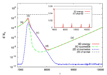
Figure 1: Evolution of the perturbation energy $E^{\prime}$ during one intermittency cycle. The total (3D) energy and the energy of 2D spanwise-independent and streamwise-independent perturbations are depicted. For comparison, the perturbation energy of 2D channel flow Jimenez (1990) is shown. Letters a to d indicate the flow stages illustrated in Fig. 2. Time is nondimensional in convective units $L/U$. Inset - evolution of perturbation energy during the entire run.

The flow transformation during one LSI cycle is presented in Figs. 1–3. Four stages can be identified. During the growth stage marked by (a), the perturbation energy is almost exclusively in the spanwise-uniform modes with wavenumber $k_{y}=0$. It can be seen in Fig. 1 that the energy of such modes shown by the short-dashed curve constitutes nearly the entire energy of perturbations. This conclusion is confirmed by 2D energy power spectra $E(k_{x},k_{y})$ (not shown) and by the fact that the Joule dissipation rate shown by long-dashed line in Fig. 3 remains at the level corresponding to dissipation of added noise. Flow fields, visualized by the streamwise velocity component in Fig. 2a, indicate that the growth phase is dominated by the classical TS mode, i.e. the exponentially growing solution of the linear stability problem of the basic flow. The growth rate $0.010752$ measured from the DNS results (branch (a) in Fig.1) agrees with $0.010976$ obtained using the linear stability code Krasnov et al. (2008a).

(a)

(b)

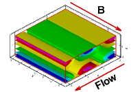
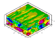
(c)

(d)

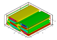
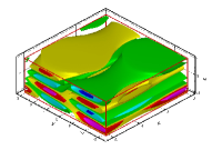
Figure 2: Flow evolution during one cycle of the intermittent process. Four stages indicated in Fig. 1 are shown using isosurfaces of streamwise velocity perturbations normalized by corresponding rms-values. (a) growing $2D$-spanwise TS mode, (b) $3D$ turbulent state at the maximum of perturbation energy, (c) decaying flow dominated by streamwise streaks, (d) disappearance of the streamwise streaks and return of the growing TS waves.

After reaching finite amplitudes, the TS mode undergoes secondary instability to 3D perturbations and disintegrates to form a turbulent state illustrated in Fig. 2b. The identification of the state as turbulent is supported by quick population of the available $k_{x}$ and $k_{y}$ wavenumbers in the energy power spectrum. The Joule dissipation rate increases sharply starting at the moment of the first 3D instability of the TS mode and eventually becomes comparable with the rate of viscous dissipation. This leads to strong suppression of the energy of perturbations and initiates the stage of decay.

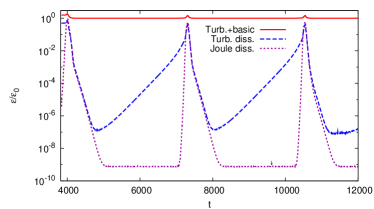
Figure 3: Evolution of viscous and magnetic dissipation rates. Total viscous dissipation (of perturbations and basic flow), viscous dissipation of perturbations only, and Joule dissipation of perturbations are shown (normalized to the dissipation $\epsilon_{0}$ of the basic flow.

The decay stage marked by (c) in Figs. 1–2 is characterized by counterintuitive and somewhat surprising behavior. Considering the nature of Joule dissipation, one could expect that the spanwise TS modes unaffected by the magnetic field would survive the suppression. This does not happen. A pattern of streamwise streaks illustrated in Fig. 2c develops as a dominant feature of the velocity perturbation field during the decay stage. The nearly streamwise-independent character of the flow is illustrated in Fig. 1, where the short-dashed curve corresponding to the energy of purely streamwise (with $k_{x}=0$) perturbations practically coincides with the curve of the total perturbation energy. The conclusion is also supported by the 2D energy spectra. The flow organization as a system of streaks, i.e. zones of enhanced or reduced streamwise velocity is visible in Fig. 2c and confirmed by the fact that during this stage the energy of the streamwise velocity component $\langle u^{\prime 2}\rangle$ is at least two orders of magnitude larger than the energy of the spanwise and wall-normal components.

We only have a simplistic explanation of the dominance of streamwise streaks during the decay stage. It is based on the presence of coherent and relatively strong streamwise streaks as a universal feature of turbulent channel flow and, in general, of turbulence with mean shear. It was shown in our recent simulations Krasnov et al. (2008b) that this feature persists in the presence of a moderate spanwise magnetic field (e.g., at $Re=10000$ and $Ha=30$). Moreover, the magnetic field renders the streaks more coherent and somewhat larger in size in all three directions by suppressing small-scale 3D perturbations. Visual indication of existence of streaks in the turbulent phase of the intermittent flow can be seen in Fig. 2b. We can assume that spanwise TS modes are completely destroyed in the turbulent flow, their energy being drained by instabilities into 3D perturbations, while the streaks form. As the 3D fluctuations are suppressed by the magnetic field, the streaks of largest spanwise wavelength (see Fig. 2c) survive as least susceptible to Joule dissipation.

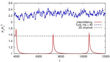
Figure 4: Mean pressure gradient (normalized to the basic flow) at $Re=8000$ for the intermittent state at $Ha=80$, for purely $2D$ channel flow Jimenez (1990), and for fully developed turbulence at $Ha=40$.

While the streamwise streaks dominate the decaying perturbation field, new spanwise modes form from the background noise. They prepare the last stage of the intermittency cycle marked by (d) in Figs. 1 and 2. It separates the decay and growth phases and is characterized by comparable energies of the growing TS mode and the decaying streaks. The total perturbation energy and the rate of viscous dissipation assume the lowest values during this stage. A change in noise level affects the initial amplitude of the TS modes, whereby the decay phase of the streaks and the growth phase of the TS mode will be correspondingly shortened or lenghtened. The typical duration of the LSI cycle was longer when round-off errors were the only noise source in our simulations.

For a long fraction of the LSI cycle the flow remains close to the Poiseuille flow, which provides the lowest friction drag for hydrodynamic channel flow. The drag experienced by 3D turbulent flow and purely 2D flow realized at lower and at higher Ha, respectively, are both on average substantially higher than for the LSI. This non-monotonous drag reduction can be seen in Fig. 4, which shows the mean pressure gradient $P_{X}$ needed to drive the flow.

The spanwise domain size $L_{y}$ could have a potentially significant effect on the LSI. Flow structures with longer spanwise wavelength experience weaker Joule disspiation, and should therefore persist up to larger values of $Ha$. The threshold for LSI could therefore be shifted to higher $Ha$ when $L_{y}$ is increased. This question and the asymptotic behavior in the limit of very large $L_{y}$ could be partly addressed by a theoretical study of secondary instabilities of growing TS modes and of decaying streamwise streaks. Our present DNS approach alone cannot provide a satisfactory answer. An experimental verification of the LSI could be attempted with the low-melting eutectic alloy In-Ga-Sn, where $Re=8000$ and $Ha=80$ would correspond to $U\sim 1\textrm{m/s}$ and $B\sim 0.3\textrm{T}$ for a channel with $L=1\textrm{cm}$. However, the rigid lateral walls in a real channel flow present an important and yet undetermined factor.

We are grateful to A. Tsinober for drawing our attention to the problem of channel flow under spanwise magnetic field, and to M. Rossi and J. Schumacher for useful comments. OZ is thankful to the Deutsche Forschungsgemeinschaft (DFG) for support of his sabbatical stay at TU Ilmenau in the framework of the Gerhard-Mercator visiting professorship program. TB, DK and AT acknowledge financial support from the DFG in the framework of the Emmy–Noether Program (grant Bo 1668/2-3). OZ’s work is supported by the grant DE FG02 03 ER46062 from the U.S. Department of Energy. Computer resources were provided by the computing centers of TU Ilmenau and of the Forschungszentrum Jülich (NIC).

References

- Davidson (1999) P. A. Davidson, Annu. Rev. Fluid Mech. 31, 273 (1999).
- Shercliff (1962) J. A. Shercliff, The Theory of Electromagnetic Flow-measurement (Cambridge University Press, 1962).
- Thess et al. (2006) A. Thess, E. Votyakov, and Y. Kolesnikov, Phys. Rev. Lett. 96, 164501 (2006).
- Moffatt (1978) H. K. Moffatt, Magnetic Field Generation in Electrically Conducting Fluids (Cambridge University Press, 1978).
- Stefani et al. (2006) F. Stefani, T. Gundrum, G. Gerbeth, G. Rüdiger, M. Schultz, J. Szklarski, and R. Hollerbach, Phys. Rev. Lett. 97, 184502 (2006).
- Zikanov and Thess (1998) O. Zikanov and A. Thess, J. Fluid Mech. 358, 299 (1998).
- Thess and Zikanov (2007) A. Thess and O. Zikanov, J. Fluid Mech. 579, 383 (2007).
- Moffatt (1967) H. K. Moffatt, J. Fluid Mech. 28, 571 (1967).
- Montgomery and Turner (1981) D. Montgomery and L. Turner, Phys. Fluids 24, 825 (1981).
- Bigot et al. (2008) B. Bigot, S. Galtier, and H. Politano, Phys. Rev. Lett. 100, 074502 (2008).
- Alemany et al. (1979) A. Alemany, R. Moreau, P. L. Sulem, and U. Frisch, J. de Mecanique 280, 18 (1979).
- Schmid and Henningson (2001) P. J. Schmid and D. S. Henningson, Stability and Transition in Shear Flows (Springer Verlag, 2001).
- Krasnov et al. (2008a) D. Krasnov, M. Rossi, O. Zikanov, and T. Boeck, J. Fluid Mech. 596, 73 (2008a).
- Jimenez (1990) J. Jimenez, J. Fluid Mech. 218, 265 (1990).
- Lee and Choi (2001) D. Lee and H. Choi, J. Fluid Mech. 429, 367 (2001).
- Krasnov et al. (2008b) D. Krasnov, O. Zikanov, J. Schumacher, and T. Boeck, Phys. Fluids 20, 095105 (2008b).