Change in Order of Phase Transitions on Fractal Lattices

Abstract

We re-examine a population model which exhibits a continuous absorbing phase transition which belongs to directed percolation in 1+1 dimensions and a first order transition in 2+1 dimensions and above. Studying the model on fractal lattices, we examine at what fractal dimension $1<d_{\rm f}<2$, the change in order occurs. As well as commenting on the order of the transitions, we produce estimates for the critical points and, for continuous transitions, some critical exponents.

Continuous nonequilibrium phase transitions continue to be an area of great interest (see Hinrichsen (2000); Lübeck (2004) for recent reviews). Perhaps the main reason for this is due to the observed universality that many such models display. As in equilibrium phase transitions, models belonging to the same universality class have identical critical exponents and the scaling functions become identical close to the critical point. By far the largest universality class of nonequilibrium phase transitions is directed percolation (DP). Indeed, it has been conjectured by Janssen and Grassberger that all models with a scalar order-parameter that exhibit a continuous phase transition from an active state to a single absorbing state belong to the class Grassberger (1982); Janssen (1981).

Most of the research on phase transitions has been conducted on lattices of integer dimension. Motivated by the apparent dependence of critical exponents on dimension, as well as topological features such as ramification and connectivity, work has also been carried out on lattices of fractal dimension $d_{\rm f}$ Jensen (1991a); Mandelbrot (1983); Pruessner et al. (2001). In this paper, we examine a model where the order of the phase transition changes from continuous to first-order for $1<d_{\rm f}<2$. We investigate the model on fractal lattices to examine at what dimension the change in order occurs $d_{{\rm f}_{\rm c}}$.

The model: In a recent paper Windus and Jensen (2007), we introduced a general population model with the reactions

$$2A+\phi\longrightarrow 3A,\quad A\longrightarrow\phi\quad\mbox{and}\quad A\phi\longleftrightarrow\phi A,$$ (1)

for an individual $A$. The model is simulated on $d$-dimensional square lattices of linear length $L$ where each site is either occupied by a single particle (1) or is empty (0). A site is chosen at random. With probability $p_{d}$ the particle on an occupied site dies, leaving the site empty. If the particle does not die, a nearest neighbour site is randomly chosen. If the neighbouring site is empty the particle moves there, otherwise, the particle reproduces with probability $p_{b}$ producing a new particle on another randomly selected neighbouring site, conditional on that site being empty. A time-step is defined as the number of lattice sites $N=L^{d}$ and periodic boundary conditions are used. Assuming spatial homogeneity, the mean field (MF) equation is easily found to be

$$\frac{\partial\rho(t)}{\partial t}=p_{\rm b}(1-p_{\rm d})\rho(t)^{2}(1-\rho(t))-p_{\rm d}\rho(t).$$ (2)

This has three stationary states,

$$\bar{\rho}_{0}=0,\quad\bar{\rho}_{\pm}=\frac{1}{2}\left(1\pm\sqrt{1-\frac{4p_{\rm d}}{p_{\rm b}(1-p_{\rm d})}}\right).$$ (3)

For $p_{\rm d}>p_{\rm b}/(4+p_{\rm b})$, $\bar{\rho}_{\pm}$ are imaginary resulting in $\bar{\rho}_{0}$ being the only real stationary state. We therefore define the critical point $p_{\rm d}=p_{\rm{d_{c}}}=p_{\rm b}/(4+p_{\rm b})$, marking the first-order phase transition between survival and extinction of the population. As we showed in our paper Windus and Jensen (2007), from monte carlo (MC) simulations, the model displays a continuous phase transition in 1+1 dimensions and belongs to DP. In higher integer dimensions, consistent with the MF prediction, the model displays a first-order phase transition. The difference in order of the phase transition between the MF and MC simulation results in 1+1 dimensions only is likely due to the larger correlations present in lower dimensions. Here, an individual is very likely to be able to find a mate on a neighbouring site. In 1+1 dimensions then, the reproduction rate is more accurately proportional to $\rho(1-\rho)$ rather than $\rho^{2}(1-\rho)$.

For the continuous phase transitions, we examined the population size $n(t)$ and survival probability $P(t)$ after beginning the simulations from a single seed - two adjacent particles. We expect the asymptotic power law behaviour Grassberger (1989)

$$n(t)\;\bar{\propto}\;t^{\eta}\quad\mbox{and}\quad P(t)\;\bar{\propto}\;t^{-\delta},$$ (4)

at the critical point. Such time-dependent simulations are known to be more efficient than steady state simulations which are also more prone to finite-size effects Jensen (1991b); Grassberger (1989). Fig. 1 a) shows the results for the (1+1)-dimensional case

a)

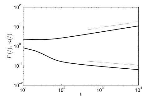
b)

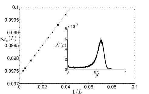
Figure 1: a) Power law behaviour at the continuous phase transition in 1+1 dimensions. The hashed lines show the DP values $\eta=0.313686$ and $\delta=0.159464$ Jensen (1999). b) The values of $p_{\rm{d_{c}}}(L)$ with the hashed line of best fit which extrapolates the data as $L\rightarrow\infty$. The inset shows the double-peaked structure at the critical point for a finite $L$.

where the gradient in the log-log plots gives the DP exponents $\eta$ and $\delta$. For the first-order phase transitions, we began our simulations from a fully-occupied lattice and observed a double-peaked structure in the histogram of population density $\mathcal{N}(\rho)$. Finding the value of $p_{\rm d}$ which equated the size of the two peaks at $\bar{\rho}_{0}$ and $\bar{\rho}_{+}$ gave the value of $p_{\rm{d_{c}}}(L)$ due to the phase coexistence that occurs at first-order transitions. Extrapolating the data as $L\rightarrow\infty$ gave a value for the critical point as shown in Fig. 1 b).

Having described how we examined our model in integer dimensions, we turn now to describing our methodology for the fractal lattices.

Methodology and results: Sierpinski carpets have been used widely to provide a generic model of fractals to study physical phenomena in fractal dimensions (see for example Gefen et al. (1980, 1983, 1984a, 1984b); Jensen (1991a); Monceau and Hsiao (2004)). They are formed by dividing a square into $l^{2}$ sub-squares and removing ($l^{2}-N_{oc})$ of these sub-squares from the centre Mandelbrot (1977). This procedure is then iterated on the remaining subsquares and repeated $\kappa$ times. As $\kappa\rightarrow\infty$ a fractal structure, denoted by $SC(l^{2},N_{oc})$, is formed. For finite $\kappa$, however, we denote the structure $SC(l^{2},N_{oc},\kappa)$ which has $N=N^{\kappa}_{oc}$ sites. The Hausdorff fractal dimension of the structure as $\kappa\rightarrow\infty$ is then $d_{\rm f}=\ln(N_{oc})/\ln(l)$. Using different values of $l$ and $N_{oc}$ enables us to use lattices of different fractal dimension $d_{\rm f}$ where $1<d_{\rm f}<2$.

Using these fractal-dimensional lattice structures, we carried out our simulations as before to determine the values for $p_{\rm{d_{c}}}$ and, where a continuous phase transition occurred, the critical exponents. For continuous phase transitions, we used time-dependent simulations, beginning from a single-seed. Here, however, the position of our initial seed may well affect the results. Two adjacent particles next to a large hole would clearly be less likely to survive than two particles surrounded by empty sites. We therefore randomly picked two adjacent sites for each run and, as before, made an average over all runs. It is also clear that, unlike before, we are unable to begin the simulations with a single-seed at the centre of the lattice due to the way in which the lattices are constructed. Due to the random position of this single-seed, we are not able to make the lattice sufficiently large so that the particles never reach the boundary. As a compromise, we use very large lattices and periodic boundary conditions. For the first-order phase transitions, we examined the histograms of population density having started from a fully-occupied lattice as described earlier. Example snapshots of both of these approaches are shown in Fig. 2.

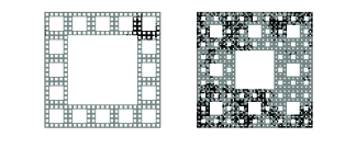
Figure 2: Snapshots of the population on the fractal lattices $SC(5^{2},16,3)$ (left) and $SC(3^{2},8,4)$. The left fractal with $d_{\rm f}=\log(16)/\log(5)\simeq 17227$ was initiated with a single seed, whereas the right lattice with $d_{\rm f}=\log(8)/\log(3)\simeq 1.8928$ began from a fully-occupied lattice.

There are many problems associated with examining critical behaviour on fractal lattices. Issues of boundary conditions and the initial location of the single seed have already been mentioned. Further, there is the obvious difficulty in the fact that finite lattices are not truly fractal. Indeed, for the histogram approach, we are required to find $p_{\rm{d_{c}}}(N)$ for different lattice sizes which we achieve by increasing $\kappa$. Such an approach, however, changes the structure of the lattice and can therefore affect the results. The effects of these difficulties and inaccuracies are minimised here since we are primarily interested in the order of the phase transition at the different dimensions.

For $d_{\rm f}\simeq 1.5573$ and $d_{\rm f}\simeq 1.7227$, we find continuous phase transitions shown by observing power law behaviour at the critical point. Plots of both $n(t)$ and $P(t)$ are shown in Fig. 3 a).

a)
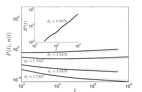
b)

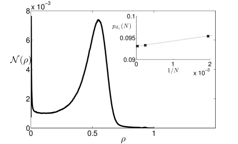
Figure 3: a) Plots of $n(t)$ and $P(t)$ at the critical point for fractal dimensions 1.5573 and 1.7227. The hashed lines give the estimated values for the exponents outlined in Tab. 1. The inset shows $R^{2}(t)$ for $d_{\rm f}\simeq 1.5573$ only. The hashed line has gradient $2/z$ where $z$ is obtained using the scaling relation (6) and the obtained values for $\eta$ and $\delta$. b) The double peaked histogram of population density indicating a first-order phase transition for $d_{\rm f}\simeq 1.8928$. The inset shows the predicted values of $p_{\rm{d_{c}}}(N)$ and an extrapolation of these results for $N\rightarrow\infty$.

For $d_{\rm f}\simeq 1.5573$, we used $SC(9^{2},32,4)$ which has just over $10^{6}$ sites. The data was obtained from over $1.6\times 10^{7}$ independent runs. Comparing the plots for this dimension with those for $d=1$, we observe significantly larger corrections to scaling. Whereas power law behaviour was obtained after $\sim 10^{2}$ time steps for the $d=1$ case, for $d_{\rm f}\simeq 1.5573$, we have to wait $\sim 10^{4}$ time steps and $\sim 10^{5}$ time steps for $d_{\rm f}\simeq 1.7227$. For this latter case, we therefore had to increase the number of time steps as well as the number of independent runs to $2.25\times 10^{8}$. The simulations took over three months of computer time on Imperial College London’s HPC HPC for each parameter value. As the crossover in the order of transition is approached, these corrections to scaling are likely to increase further in size. This, then, represents a further challenge in obtaining accurate values for the critical points and exponents as $d_{\rm f}\rightarrow d_{{\rm f}_{\rm c}}$.

From the other end of the interval $1<d_{\rm f}<2$, for $d_{\rm f}\simeq 1.8928$, no power law behaviour was observed, rather, the double-peaked structure of the histogram of population density. To increase the size of our lattice, we increased the value of $\kappa$ and found the value of $p_{\rm{d_{c}}}(N)$ for each case. Extrapolating the results for infinite system size, we obtained an approximation for the critical point as shown in Fig. 3 b).

For $d_{\rm f}\simeq 1.7925$,

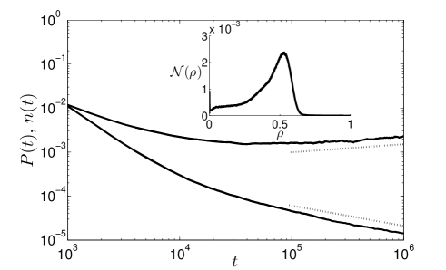
Figure 4: Possible power law behaviour for $d_{\rm f}\simeq 1.7927$. The inset shows the lack of the double-peaked structure.

the histogram plots do not show the double-peaked structure close to the critical point. Plots of $n(t)$ and $P(t)$ appear to show power law behaviour, but with very large corrections to scaling. The plots shown in Fig. 4 required over $5\times 10^{8}$ runs, taking over six months of computer time. On closer inspection, the values of $\eta=0.19$ and $\delta=0.46$ that we obtained at this dimension appear to be unlikely. Both vales are the wrong side of the DP values for $d=2$, indicating that the plots actually show supercritical behaviour. Due to the large amounts of time required to produce such plots, we predict that the phase transition is continuous for $d_{\rm f}\simeq 1.7925$ but are, now at least, unable to provide strong evidence for this.

A summary of our results at the different dimensions are outlined in Tab. 1.

$d_{\rm f}$	$SC(l^{2},N_{oc},\kappa)$	Order of	$p_{\rm{d_{c}}}$	$\delta$	$\eta$
		phase transition		(if applicable)	(if applicable)
1		continuous	0.071754	0.160	0.313
$\log(32)/\log(9)\simeq 1.5573$	$SC(9^{2},32,4)$	continuous	0.08553	0.30	0.29
$\log(16)/\log(5)\simeq 1.7227$	$SC(5^{2},16,6)$	continuous	0.08819	0.39	0.24
$\log(12)/\log(4)\simeq 1.7925$	$SC(4^{2},12,6)$	?	?	?	?
$\log(8)/\log(3)\simeq 1.8928$	$SC(3^{2},8,3/4/5)$	first-order	0.093	n/a	n/a
2		first-order	0.0973	n/a	n/a

Table 1: Summary of the results. The data for $d=1,2$ was obtained in Windus and Jensen (2007). Due to the large corrections to scaling, we were unable to provide strong evidence for the order of the phase transition for $d_{\rm f}\simeq 1.7925$. While we predict it to be continuous, we leave this row with question marks due to our uncertainty.

For the continuous phase transitions, a generally accepted approach of obtaining more accurate values for the critical exponents is by examining the local slopes (see for example Grassberger (1989)). For such an approach we plot, for example, $\delta(t)$ against $1/t$ where

$$-\delta(t)=\frac{\ln\left[P(t)/P(t/m)\right]}{\ln(m)},$$ (5)

and $m$ is the local range over which the slope is measured. Due to the previously mentioned large corrections to scaling we observed, such an approach did not yield accurate results. For the method to work properly, the number of time steps over which the data was collected would have to be raised significantly, increasing the required computer time further. The values for the exponents that we obtained then were estimated only by measurement of the gradient of the above plots and are therefore accurate to only $\pm 0.005$.

A check for the consistency of the exponents can be obtained by the scaling relations. From the scaling relation Grassberger (1989)

$$\eta+2\delta=d/z,$$ (6)

we can check our values of $\eta$ and $\delta$ using the fractal dimension for $d$ and obtaining the dynamical exponent $z=\nu_{\parallel}/\nu_{\perp}$. This exponent can be obtained by examining the mean square distance of spread from the initial seed of the population $R^{2}(t)$ averaged over surviving runs only. At the critical point, we expect the asymptotic power law behavior $R^{2}(t)\;\bar{\propto}\;t^{2/z}$ Grassberger (1989). For $d_{\rm f}=1.5573$ we show the results in the inset of Fig. 3 a) where we plot $R^{2}(t)$ along with $t^{2/z}$ using the value of $z$ obtained from the scaling relation (6) given by the obtained values for $\eta$ and $\delta$. We see very good agreement between the exponents. For larger dimensions, however, the crossover effects render, in particular $R^{2}(t)$, inaccurate. Oscillations in $R^{2}(t)$, perhaps due to the fractal structure, delay the power-law behaviour to large values of $t$ that are impractical to simulate.

Remarks: Having examined our model in different fractal dimensions, we found that the dimension at which the order of the phase transition changes is in the range $1.7227<d_{{\rm f}_{\rm c}}<1.8928$. We predict the lower bound of this range to be more accurately given by $1.7927$ but offer no firm proof. We predict that below $d_{{\rm f}_{\rm c}}$ the larger correlations between the particles ensure that a continuous phase transition is observed.

This present study was limited by the available computer power (over two years of processing time was required in total). Due to the large corrections to scaling, it was difficult to obtain truly accurate results for the critical points and exponents in the continuous regime. Given more computer time, we would be able to run the simulations over a greater number of time steps to increase the accuracy. Further, it would also be interesting to examine if the values of the critical points and exponents depend on the type of fractal lattices used.

References

- Hinrichsen (2000) H. Hinrichsen, Adv. Phys. 49, 815 (2000).
- Lübeck (2004) S. Lübeck, Int. J. Mod. Phys. B 18, 3977 (2004).
- Grassberger (1982) P. Grassberger, Z. Phys. B 47, 365 (1982).
- Janssen (1981) H. K. Janssen, Z. Phys. B 42, 151 (1981).
- Jensen (1991a) I. Jensen, J. Phys. A: Math. Gen. 24, L1111 (1991a).
- Mandelbrot (1983) B. Mandelbrot, The Fractal Geometry of Nature (W.H. Freeman and Company, New York, 1983).
- Pruessner et al. (2001) G. Pruessner, D. Loison, and K.D. Schotte, Phys. Rev. B 64, 134414 (2001).
- Windus and Jensen (2007) A. Windus and H. Jensen, J. Phys. A: Math. Theor. 40, 2287 (2007).
- Grassberger (1989) P. Grassberger, J. Phys. A: Math. Gen. 22, 3673 (1989).
- Jensen (1991b) I. Jensen, Phys. Rev. A 43, 3187 (1991b).
- Jensen (1999) I. Jensen, J. Phys. A: Math. Gen. 32, 5233 (1999).
- Gefen et al. (1980) Y. Gefen, B.B. Mandelbrot, and A. Aharony, Phys. Rev. Lett. 45, 855 (1980).
- Gefen et al. (1983) Y. Gefen, A. Aharony, and B. Mandelbrot, J. Phys. A: Math. Gen. 16, 1267 (1983).
- Gefen et al. (1984a) Y. Gefen, A. Aharony, Y. Shapir, and B. Mandelbrot, J. Phys. A: Math. Gen. 17, 435 (1984a).
- Gefen et al. (1984b) Y. Gefen, A. Aharony, and B. Mandelbrot, J. Phys. A: Math Gen. 17, 1277 (1984b).
- Monceau and Hsiao (2004) P. Monceau and P.Y. Hsiao, Phys. Lett. A 332, 310 (2004).
- Mandelbrot (1977) B. Mandelbrot, Fractals: Form, Chance and Dimension (Freeman, New York, 1977).
- (18) www.imperial.ac.uk/ict/services/teachingandresearchservices/highperformancecomputing.