Stochastic modeling of chaotic masonry via mesostructural characterization

Abstract.

The purpose of this study is to explore three numerical approaches to the elastic homogenization of disordered masonry structures with moderate meso/macro-lengthscale ratio. The methods investigated include a representative of perturbation methods, the Karhunen-Loève expansion technique coupled with Monte-Carlo simulations and a solver based on the Hashin-Shtrikman variational principles. In all cases, parameters of the underlying random field of material properties are directly derived from image analysis of a real-world structure. Added value as well as limitations of individual schemes are illustrated by a case study of an irregular masonry panel.

Keywords

irregular masonry structures; stochastic homogenization; two-point statistics; improved perturbation methods; Karhunen-Loève expansion; Hashin-Shtrikman variational principles

1. Introduction

The last decade has witnessed rapid advances in modelling and simulation of masonry structures, mainly in connection with reconstruction and rehabilitation of historical monuments. The major impetus for these developments came from a seminal contribution by Anthoine [1], which clearly demonstrated that the complex overall behavior of elastic regular masonry can be systematically addressed in the framework of homogenization theory for periodic heterogeneous media. These results were subsequently extended towards tools capable of predicting non-linear response of masonry structures with deterministic geometry and sufficiently small ratio between the characteristic size of masonry bond (mesoscale) and the structural level (macroscale), see [25, 28] for an extensive overview of the field. Both these assumptions, however, may show to be inadequate for historical structures, where the spatial distribution of individual constituents is random rather then deterministic and the typical size of a block may well become comparable to the macroscopic lengthscale.

When adopting certain simplifying assumptions, a vast body of approaches is currently available for the treatment of irregular masonry as a random heterogeneous material. Under the hypothesis of widely separated lengthscales, the well-established tools of stochastic continuum micromechanics can be adopted, in which the inhomogeneous body in question is replaced with a homogeneous equivalent with properties determined from analysis of a representative volume element, locally replacing the mesoscale level, see monographs [5, 41] for up-to-date reviews. To the authors’ best knowledge, the only masonry-related study available in this field was presented by Šejnoha et al. [43] in the framework of stochastic re-formulation of Hashin-Shtrikman variational principles due to Willis [44]. Additionally, the notion of a stochastic representative element can be adopted, based either on matching spatial statistics as originally proposed by Povirk in [32] and subsequently applied to masonry structures in [43, 48], or deduced from the convergence of apparent macroscopic properties. The latter concept was proposed by Huet [17] in the deterministic setting, extended by Sab [34] to random media and implemented for historical masonry structures by Cluni and Gusella [7, 14].

Complementary, systems with random material properties quantified by random variables and deterministic (or slightly perturbed) geometry of the representative volume can be treated employing numerical techniques of stochastic mechanics such as Monte-Carlo simulations [20], perturbation-based methods [22, 35] or approaches based on an empirical probability distribution function [36]; see also [21] for a systematic overview. Most generally, uncertainties in spatial distribution and material properties of individual phases can be jointly characterized when resorting to random field description [42]. Under suitable assumptions on the underlying random field, a rigorous homogenization theory available in [3, 19] was used to construct efficient stochastic homogenization solvers, based on spectral collocation methods [18] or Fourier-Galerkin approaches [46, 47]. Recently, these methods were extended by Xu [45] to treat heterogeneous media with small but finite lengthscale contrast.

Finally, as the macro/meso scale ratio further increases, the rapidly developing tools of Stochastic Finite Element (SFE) methods [2, 13, 30, 40] become applicable for the assessment of overall response. It should be emphasized that even though the random field description definitely offers a more general framework than the alternative schemes, its major weakness is that the random field is often introduced without a clear link with the heterogeneous mesostructure, see [6] for a lucid discussion on the topic. Moreover, the application of the random field/variable paradigms to the simulation of masonry structure seems to be currently missing; the only related works the authors are aware of is a recent contribution of Spence et al. [39] dealing with mesostructure generation of irregular masonry walls.

In this contribution, three numerical approaches to the determination of the overall response of elastic masonry with comparable macro- and meso-lengthscales are presented. A unifying feature is the description of mechanical properties in the form of a random field with the second-order statistics consistently derived from image analysis of the investigated structure. In Section 2, this procedure is briefly summarized following the exposition of Falsone and Lombardo [10]. The second level of representation involves the determination of basic statistics related to the response of a finite size heterogeneous masonry structure. In particular, the improved perturbation method is introduced first in Section 3, followed in Section 4 by the Monte-Carlo approach with individual realizations of the random field generated using the Karhunen-Loève expansion. Section 5 is concerned with the application of the Hashin-Shtrikman variational principles, coupled with the Finite Element discretization to allow for the treatment of finite-size bodies. In Section 6, the results obtained with the selected methods are mutually compared on the basis of elastic analysis of an irregular masonry panel. Finally, Section 7 introduces possible extensions and refinements of the studied approaches.

In the following text, the Voigt representation of symmetric tensorial quantities is systematically employed, see e.g. [4]. In particular, $a$, ${\boldsymbol{a}}$ and ${\boldsymbol{A}}$ denote a scalar value, a vector or a matrix representation of a second-order tensor and a matrix representation of a fourth-order tensor, respectively.

2. Probabilistic characterization of material property via mesostructural statistics

Before getting to the heart of the matter, we begin by summarizing essential terminology related to the theory of random fields [42]. Given a complete probability space $\{\Theta,\mathcal{F},\mathcal{P}\}$ with sample space $\Theta$, $\sigma$-algebra $\mathcal{F}$ on $\Theta$ and probability measure $\mathcal{P}$ on $\mathcal{F}$, a scalar random field $H$ defined on an open set $\Omega\subset{\mathbb{R}}^{d}$ is a mapping

$$H:\Theta\times\Omega\rightarrow{\mathbb{R}},$$ (1)

such that, for every ${\boldsymbol{x}}\in\Omega$, $H({\boldsymbol{x}};\theta)$ is a random variable with respect to the triple $\{\Theta,\mathcal{F},\mathcal{P}\}$. The mean of a random field is then given as

$$\mu_{H}({\boldsymbol{x}})={\mathbb{E}}\left[H({\boldsymbol{x}};\theta)\right]=\int_{\Theta}H({\boldsymbol{x}};\theta)\,{\mathrm{d}}\mathcal{P}(\theta),$$ (2)

for any ${\boldsymbol{x}}\in\Omega$, whereas the covariance of two random fields $H$ and $G$ is defined by

$$R_{HG}({\boldsymbol{x}},{\boldsymbol{x}}^{\prime})={\mathbb{E}}\left[\left(H({\boldsymbol{x}};\theta)-\mu_{H}({\boldsymbol{x}})\right)\left(G({\boldsymbol{x}}^{\prime};\theta)-\mu_{G}({\boldsymbol{x}}^{\prime})\right)\right],$$ (3)

with the symbol $R_{H}({\boldsymbol{x}},{\boldsymbol{x}}^{\prime})=R_{HH}({\boldsymbol{x}},{\boldsymbol{x}}^{\prime})$ reserved for the autocovariance, reducing to a variance for ${\boldsymbol{x}}={\boldsymbol{x}}^{\prime}$:

$$\sigma_{H}^{2}({\boldsymbol{x}})={\mathbb{E}}\left[\left(H({\boldsymbol{x}};\theta)-\mu_{H}({\boldsymbol{x}})\right)^{2}\right].$$ (4)

A random field $H({\boldsymbol{x}};\theta)$ is said to be homogeneous if all its joint probability distribution functions (PDFs) remain invariant under the translation of the coordinate system, leading to substantial simplification of the considered statistics:

$$\mu_{H}({\boldsymbol{x}})=\mu_{H}=\mbox{const}, \sigma_{H}^{2}({\boldsymbol{x}})=\sigma_{H}^{2}=\mbox{const}, R_{H}({\boldsymbol{x}},{\boldsymbol{x}}^{\prime})=R_{H}({\boldsymbol{x}}-{\boldsymbol{x}}^{\prime}).$$ (5)

Assuming that the autocovariance function can be well-approximated by an exponential function, the correlation length $\lambda_{H}$ is defined by means of inequality:

$$\forall\|{\boldsymbol{x}}-{\boldsymbol{x}}^{\prime}\|\geq\lambda_{H}:R_{H}({\boldsymbol{x}}-{\boldsymbol{x}}^{\prime})\leq\frac{\sigma_{H}^{2}}{\exp(1)},$$ (6)

hence quantifying the characteristic dimension of the spatial fluctuations. Finally, a random field is ergodic if all information on joint PDFs are available from a single realization of the field.

With reference to the quantification of morphology of random heterogeneous materials, variable $\theta$ simply denotes a realization of random mesostructure drawn from the ensemble space $\Theta$ of all admissible configurations. Of particular importance is the characteristic function related to the spatial distribution of the $i$-th phase:

$$\chi^{(i)}({\boldsymbol{x}};\theta)=\left\{\begin{array}[]{cl}1&\mbox{if }{\boldsymbol{x}}\in\Omega^{(i)}(\theta),\\ 0&\mbox{otherwise},\end{array}\right.$$ (7)

where $\Omega^{(i)}(\theta)$ is the domain occupied by the $i$-th phase for realization $\theta$ and $i$ can take values $\{s,m\}$, where $s$ denotes the stone phase and $m$ refers to the mortar phase. The characteristic functions of individual phases are not independent, once e.g. the “stone” characteristic function is provided, the complementary descriptor follows from

$$\chi^{(m)}({\boldsymbol{x}};\theta)+\chi^{(s)}({\boldsymbol{x}};\theta)=1.$$ (8)

Therefore, we concentrate on the stone phase in the sequel.

When assuming the statistically uniform and ergodic media, the basic spatial statistics is provided by

$$\mu_{\chi^{(s)}}=c^{(s)}, R_{\chi^{(s)}}({\boldsymbol{x}}-{\boldsymbol{x}}^{\prime})=S^{(s)}_{2}({\boldsymbol{x}}-{\boldsymbol{x}}^{\prime})-\left(c^{(s)}\right)^{2},$$ (9)

where $c^{(s)}$ is the volume fraction of the relevant phase and $S^{(s)}_{2}$ coincides with the two-point probability function, defined for generic phases $i,j\in\{s,m\}$ as [41]

$$S^{(ij)}_{2}({\boldsymbol{x}},{\boldsymbol{x}}^{\prime})={\mathbb{E}}\left[\chi^{(i)}({\boldsymbol{x}};\theta)\chi^{(j)}({\boldsymbol{x}}^{\prime};\theta)\right],$$ (10)

hence quantifying the probability of two points ${\boldsymbol{x}}$ and ${\boldsymbol{x}}^{\prime}$ being located in phases $i$ and $j$ (with $S^{(i)}_{2}$ abbreviating $S^{(ii)}_{2}$).

The statistical descriptors of real mesostructures can be evaluated on the basis of a digitized images of the sample, leading to the discretization of the characteristic function in terms of an $N_{x}\times{N_{y}}$ bitmap. Replacing the point coordinate $(x,y)$ by the pixel $(i,j)$ located in the $i$-th row and the $j$-th column, the characteristic function is defined by the discrete value $\chi_{s}(i,j)$. The estimates of one-point and two-point correlation functions, under the periodic boundary condition, follow from relations (see, e.g., [11])

$$c^{(s)} \approx \frac{1}{N_{x}N_{y}}\sum_{i=1}^{N_{x}}\sum_{j=1}^{N_{y}}\chi^{(s)}(i,j),$$ (11)

$$S^{(s)}_{2}(m,n) \approx \frac{1}{N_{x}N_{y}}\sum_{i=1}^{N_{x}}\sum_{j=1}^{N_{y}}\chi^{(s)}(i,j)\chi^{(s)}(1+(i+m)\%N_{x},1+(j+n)\%N_{y}),$$ (12)

where $m$ and $n$ are distances between two generic points measured in pixels and $a\%b$ denotes $a$ modulo $b$. Note that the sums (11) and (12) can be efficiently evaluated using the Fast Fourier transform techniques; see e.g. [41]. To automate the acquisition of these functions, a software working in MATLAB was implemented [10], covering all the basic steps of mesostructure quantification with the data provided in the form of a color image, see Figure 1 for an illustration of the procedure.

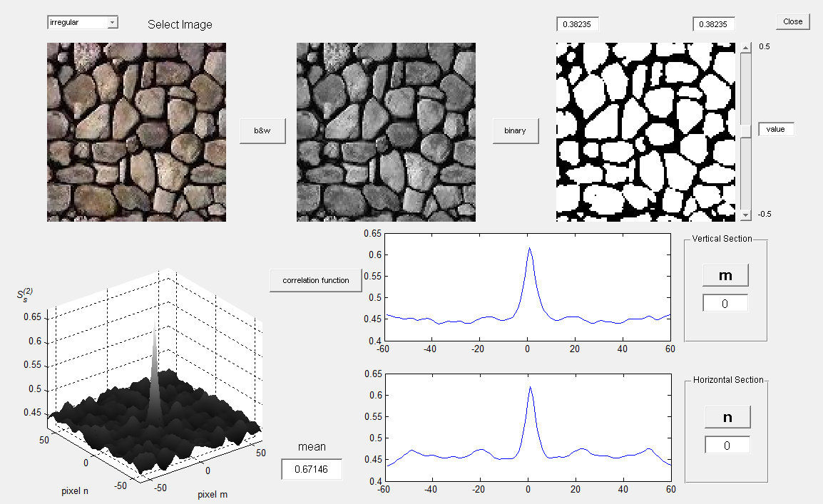
Figure 1. Example of the program used to obtain correlation function for a chaotic masonry panel (San Marco d’Alunzio, Italy).

Apart from providing basic spatial statistics of random mesostructure, the phase characteristic functions allow us to directly express the matrix-valued field of material properties in the form

$${\boldsymbol{C}}({\boldsymbol{x}};\theta)=\chi^{(s)}({\boldsymbol{x}};\theta){\boldsymbol{C}}^{(s)}+\chi^{(m)}({\boldsymbol{x}};\theta){\boldsymbol{C}}^{(m)}={\boldsymbol{C}}^{(m)}+\chi^{(s)}({\boldsymbol{x}};\theta)({\boldsymbol{C}}^{(s)}-{\boldsymbol{C}}^{(m)}),$$ (13)

where ${\boldsymbol{C}}^{(s)}$ and ${\boldsymbol{C}}^{(m)}$ are the deterministic material stiffness matrices of the two constituents. The mean and the covariance functions then follow from Equations (2) and (3):

$$\mu_{C_{ij}}({\boldsymbol{x}}) = C_{ij}^{(m)}+c^{(s)}(C_{ij}^{(s)}-C_{ij}^{(m)}),$$ (14)

$$R_{C_{ij}C_{kl}}({\boldsymbol{x}}-{\boldsymbol{x}}^{\prime}) = R_{\chi^{(s)}}({\boldsymbol{x}}-{\boldsymbol{x}}^{\prime})\left(C_{ij}^{(s)}-C_{ij}^{(m)}\right)\left(C_{kl}^{(s)}-C_{kl}^{(m)}\right).$$ (15)

A similar representation is available when phase properties become random variables, see [10] for additional discussion.

3. Improved perturbation method

Consider a mechanical system with the randomness in material properties specified in terms of the random field $\chi^{(s)}({\boldsymbol{x}};\theta)$. In the context of finite element analysis of static problems, the discretized form of equilibrium equations reads [4]

$${\boldsymbol{K}}_{h}(\chi^{(s)}({\boldsymbol{x}};\theta)){\boldsymbol{u}}_{h}(\theta)={\boldsymbol{F}}_{h},$$ (16)

where $h$ is a characteristic element size, the force vector ${\boldsymbol{F}}_{h}$ is assumed to be deterministic and the global stiffness matrix ${\boldsymbol{K}}_{h}$ is stochastic due to uncertainty in the material properties, which makes the nodal displacement vector ${\boldsymbol{u}}_{h}$ non-deterministic as well.

To handle the random field in Eq. (16) computationally, an appropriate discretization technique in the stochastic variable has to be used. In this work, the widely used mid-point method is employed to represent the random field consistently with the underlying finite element mesh. Therefore, two different considerations control the size of an element $h$, cf. [2]. The first one comprises the usual “deterministic” criteria, where the mesh size is governed by expected stress gradients and geometry. The additional requirement is linked with the correlation length $\lambda_{\chi^{(s)}}$; the distance between two adjacent random variables has to be short enough to capture the essential features of the random field. The general recommendation is to choose $2h\approx\lambda_{\chi^{(s)}}$ to describe the stochastic field with sufficient accuracy [29].

In the current implementation, the value at the element center is used to characterize the stochastic field, thus yielding a representation in the form of a vector of random variables

$${\boldsymbol{\chi}}^{(s)}_{h}(\theta)=\left[\begin{array}[]{cccc}\chi^{(s)}_{h,1}(\theta)&\chi^{(s)}_{h,2}(\theta)&\ldots&\chi^{(s)}_{h,N_{e}}(\theta)\end{array}\right]{\sf{}^{T}},$$ (17)

with $\chi^{(s)}_{h,e}(\theta)$ being the value of $\chi^{(s)}({\boldsymbol{x}};\theta)$ at the $e$-th element centroid and $N_{e}$ denoting the number of elements. The element stiffness matrix is calculated from the standard finite element methodology and is expressed as [4]

$${\boldsymbol{K}}_{h,e}\left(\chi^{(s)}_{h,e}(\theta)\right)=\int_{\Omega_{e}}{\boldsymbol{B}}_{h,e}{\sf{}^{T}}({\boldsymbol{x}}){\boldsymbol{C}}_{e}\left(\chi^{(s)}_{h,e}(\theta)\right){\boldsymbol{B}}_{h,e}({\boldsymbol{x}})\,{\mathrm{d}}{\boldsymbol{x}},$$ (18)

where ${\boldsymbol{B}}_{h,e}$ is the deterministic displacement-to-strain matrix related to the $e$-th element and the material stiffness matrix ${\boldsymbol{C}}_{e}$ follows from Eq. (13). After the assembly procedure, the global form of equilibrium equations becomes

$${\boldsymbol{K}}_{h}({\boldsymbol{\chi}}^{(s)}_{h}(\theta)){\boldsymbol{u}}_{h}(\theta)={\boldsymbol{F}}_{h}.$$ (19)

Among the various perturbative SFE approaches proposed in literature, an improved perturbation technique proposed by Elishakoff et al. [9] is employed in this work. When compared to the traditional first-order expansion schemes, the added value of the adopted method is that the mean value of the response variables depends on the covariance information on uncertain input parameters, thereby optimally utilizing the available second-order statistics, see also [24, Chapter 5] for further discussion. Following this approach, the mean of the response vector ${\boldsymbol{u}}_{h}$ is given by

$${\boldsymbol{\mu}}_{{\boldsymbol{u}}_{h}}={\boldsymbol{A}}_{h}^{-1}{\boldsymbol{F}}_{h},$$ (20)

where

$${\boldsymbol{A}}_{h}={\boldsymbol{K}}_{h,0}-\sum_{i=1}^{N_{e}}\sum_{j=1}^{N_{e}}R_{\chi^{(s)}_{i}\chi^{(s)}_{j}}{\boldsymbol{K}}_{h,i}^{\prime}\left({\boldsymbol{K}_{h,0}}^{-1}\right){\boldsymbol{K}}_{h,j}^{\prime},$$ (21)

with the stiffness matrix sensitivities provided by

$${\boldsymbol{K}}_{h,0}={\boldsymbol{K}}_{h}({\boldsymbol{\chi}}^{(s)}_{h})\Bigr{|}_{{\boldsymbol{\chi}}^{(s)}_{h}={\mathbb{E}}\left[{\boldsymbol{\chi}}^{(s)}_{h}\right]}, {\boldsymbol{K}}^{\prime}_{h,i}=\frac{\partial{\boldsymbol{K}}_{h}({\boldsymbol{\chi}}^{(s)}_{h})}{\partial\chi^{(s)}_{h,i}}\Bigr{|}_{{\boldsymbol{\chi}}^{(s)}_{h}={\mathbb{E}}\left[{\boldsymbol{\chi}}^{(s)}_{h}\right]}.$$ (22)

In addition, the autocovariance matrix of displacements follows from

$${\boldsymbol{R}}_{{\boldsymbol{u}}_{h}}={\boldsymbol{K}}_{0,h}^{-1}{\boldsymbol{C}}_{h}{\boldsymbol{K}_{0,h}}^{-1},$$ (23)

where

$${\boldsymbol{C}}_{h}=\sum_{i=1}^{N_{e}}\sum_{j=1}^{N_{e}}R_{\chi^{(s)}_{i}\chi^{(s)}_{j}}{\boldsymbol{K}}_{h,i}^{\prime}{\boldsymbol{\mu}}_{{\boldsymbol{u}}_{h}}\left({\boldsymbol{\mu}}_{{\boldsymbol{u}}_{h}}\right){\sf{}^{T}}{\boldsymbol{K}}_{j}^{\prime},$$ (24)

see [9] for additional details.

4. Karhunen-Loève expansion

The application of Karhunen-Loève expansion (KLE) to stochastic boundary value problems has been pioneered by Ghanem and his co-workers [12, 13] and provides an alternative way to random field generation. The KLE can be seen as a special case of the orthogonal series expansion where the orthogonal functions are chosen as the eigenfunctions of a Fredholm integral equation of the second kind with autocovariance as kernel [49].

With reference to the mesostructure-based random fields considered in the current work, we start from the KLE of the characteristic function $\chi^{(s)}({\boldsymbol{x}};\theta)$ in the form

$$\chi^{(s)}({\boldsymbol{x}};\theta)=\mu_{\chi^{(s)}}({\boldsymbol{x}})+\sum_{i=1}^{\infty}\sqrt{\lambda_{i}}\xi_{i}(\theta)f_{i}({\boldsymbol{x}}),$$ (25)

where $\lambda_{i}$ and $f_{i}({\boldsymbol{x}})$ are the eigenvalues (decreasing in magnitude) and eigenfunctions of the autocovariance $R_{\chi^{(s)}}({\boldsymbol{x}},{\boldsymbol{x}}^{\prime})$, $\{\xi_{i}(\theta)\}$ is a set of random variables [40]. Note that the use of KLE is limited to the representation of input random fields as the covariance structure needs to be specified a priori. Since the kernel $R_{\chi^{(s)}}({\boldsymbol{x}},{\boldsymbol{x}}^{\prime})$ is bounded, symmetric and non-negative, it has all eigenfunctions mutually orthogonal and forming a complete set spanning the function space to which $\chi^{(s)}({\boldsymbol{x}};\theta)$ belongs. Therefore, the autocovariance function can be decomposed into

$$R_{\chi^{(s)}}({\boldsymbol{x}},{\boldsymbol{x}}^{\prime})=\sum_{i=1}^{\infty}\lambda_{i}f_{i}({\boldsymbol{x}})f_{i}({\boldsymbol{x}}^{\prime}),$$ (26)

with eigenfunctions $f_{i}({\boldsymbol{x}})$ and eigenvalues $\lambda_{i}$ found as the solutions of the homogeneous Fredholm integral equation of the second kind

$$\int_{\Omega}R_{\chi^{(s)}}({\boldsymbol{x}},{\boldsymbol{x}}^{\prime})f_{i}({\boldsymbol{x}}^{\prime})\,{\mathrm{d}}{\boldsymbol{x}}^{\prime}=\lambda_{i}f_{i}({\boldsymbol{x}}).$$ (27)

The parameter $\xi_{i}(\theta)$ in Eq. (25) corresponds to an uncorrelated standardized random variable expressed as

$$\xi_{i}(\theta)=\frac{1}{\sqrt{\lambda_{i}}}\int_{\Omega}\big{[}\chi^{(s)}({\boldsymbol{x}};\theta)-\mu_{\chi^{(s)}}({\boldsymbol{x}})\big{]}f_{i}({\boldsymbol{x}})\,{\mathrm{d}}{\boldsymbol{x}}.$$ (28)

The most important aspect of the representation (25) is that the fluctuations are decomposed into a set of deterministic functions in the spatial variables separately multiplying purely random coefficients.

In practical implementations, the series (25) and (26) are truncated after $M$ terms, yielding the approximations

$$\chi^{(s)}({\boldsymbol{x}};\theta) \approx \mu_{\chi^{(s)}}({\boldsymbol{x}})+\sum_{i=1}^{M}\sqrt{\lambda_{i}}\xi_{i}(\theta)f_{i}({\boldsymbol{x}}),$$ (29)

$$R_{\chi^{(s)}}({\boldsymbol{x}},{\boldsymbol{x}}^{\prime}) \approx \sum_{i=1}^{M}\lambda_{i}f_{i}({\boldsymbol{x}})f_{i}({\boldsymbol{x}}^{\prime}).$$ (30)

Such spatial semi-discretization is optimal in the sense that the mean square error resulting from a truncation after the $M$-th term is minimized [13].

The efficiency of KLE for simulating random fields crucially hinges on accurate eigenvalues and eigenfunctions of the covariance kernel. In this paper, the Galerkin method with orthogonal polynomial basis functions is employed to solve the Fredholm equation (27) for general domains and autocovariance functions, see [24, Chapter 7] for implementation details. In addition, a careful convergence study of truncated KLE presented in [16] has demonstrated, for specific classes of stochastic fields, the dependence of the optimal value of $M$ on the ratio of the characteristic domain length $L$ to the correlation parameter $\lambda_{\chi^{(s)}}$. For weakly correlated processes ($\lambda_{\chi^{(s)}}/L\ll 1$), the higher order eigenvalues cannot be neglected without having a serious impact on the accuracy of the simulation.

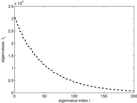
Figure 2. Distribution of eigenvalues for KLE related to chaotic masonry sample.

Such behavior is illustrated by means of Figure 2, showing the decay of eigenvalues of KLE with the covariance kernel determined for the masonry sample presented in Section 2. In addition, several associated eigenfunctions are collected in Figure 3. Clearly, the random field under consideration is weakly correlated as $\lambda_{\chi^{(s)}}/L\approx 10/120$, see Figure 1, and a large number of terms ($M\approx 200$) is needed to capture fine features of the covariance, cf. Figure 3(d).

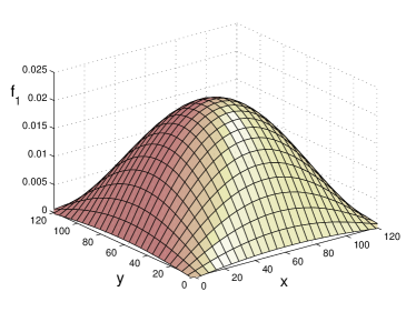
(a)

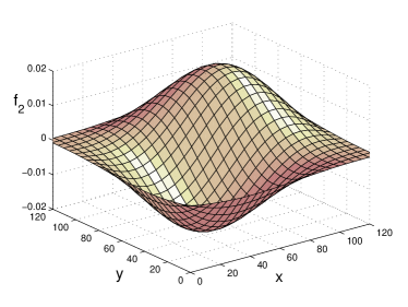
(b)

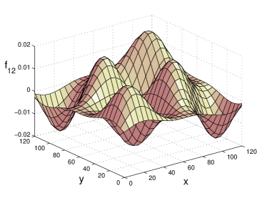
(c)

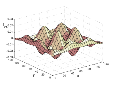
(d)

Figure 3. Examples of eigenfunctions $f_{i}$; (a) $i=1$, (b) $i=2$, (c) $i=12$, (d) $i=24$.

With a KLE of the spatial autocovariance function at hand, the individual realizations of the heterogeneous body can be efficiently generated once an appropriate model for the random field $\chi^{(s)}({\boldsymbol{x}};\theta)$ is adopted. In the current study, we assume that the random field is Gaussian, for which the coefficients $\xi_{i}(\theta)$ in Eq. (28) become independent standard Gaussian variables of zero mean and unit variance. It should be emphasized that the assumption of Gaussian form of characteristic function is somehow questionable for binary heterogeneous media, where the log-normal or beta probability densities appear to be more appropriate to reflect the intrinsic discreteness of the random field. The Gaussian assumption is adopted here mainly due to simplicity of the resulting simulation algorithm based on well-established routines, see also related works [6, 45, 46] for further discussion.

The final step of the KLE-based solver involves the determination of the response statistics for a structure with material stiffness determined from Eq. (13):

$${\boldsymbol{C}}({\boldsymbol{x}};\theta)\approx{\boldsymbol{C}}^{(m)}+\left(c^{(s)}+\sum_{i=1}^{M}\sqrt{\lambda_{i}}\xi_{i}(\theta)f_{i}({\boldsymbol{x}})\right)({\boldsymbol{C}}^{(s)}-{\boldsymbol{C}}^{(m)}).$$ (31)

The frequently adopted framework of spectral SFE [13, 30], where the response variable is discretized using the polynomial chaos expansion in the stochastic coordinate, is not applicable in the current case as the high number of KLE terms results in unmanageable number of polynomial chaos components. Therefore, similarly to e.g. [23, 37], a direct Monte-Carlo approach is adopted in the present study, leading to a simulation procedure summarized in Figure 4. Note that in the FE analysis, the characteristic element size $h$ has to verify $2h\leq\lambda_{{}^{(s)}}$ again to correctly reproduce the autocovariance function.

Figure 4. Overview of the Monte-Carlo simulation coupled with KLE.

Once the sampling phase is completed, the unbiased mean and covariance of displacement vectors are provided by

$${\boldsymbol{\mu}}_{{\boldsymbol{u}}_{h}} = \frac{1}{n}\sum_{j=1}^{n}{\boldsymbol{u}}_{h}(\theta_{j}),$$ (32)

$${\boldsymbol{R}}_{{\boldsymbol{u}}_{h}} = \frac{1}{n-1}\sum_{j=1}^{n}\left[{\boldsymbol{u}}_{h}(\theta_{j})\left({\boldsymbol{u}}_{h}(\theta_{j})\right){\sf{}^{T}}-n{\boldsymbol{\mu}}_{{\boldsymbol{u}}_{h}}\left({\boldsymbol{\mu}}_{{\boldsymbol{u}}_{h}}\right){\sf{}^{T}}\right],$$ (33)

where, in accord with Figure 4, $n$ denotes the number of simulations and $\theta_{j}$ is used to denote the $j$-th deterministic realization.

5. Hashin-Shtrikman variational approach

The last approach investigated here builds on the classical Hashin-Shtrikman variational principles for the heterogeneous media [15], extended to the stochastic setting by Willis [44]. The basic idea of the method is the introduction of a reference homogeneous body with stiffness tensor ${\boldsymbol{C}}_{0}$, employed in the analysis instead of an inhomogeneous realization ${\boldsymbol{C}}({\boldsymbol{x}};\theta)$, recall Eq. (13). The heterogeneity of the material is compensated using the polarization stress ${\boldsymbol{\tau}}({\boldsymbol{x}};\theta)$, resulting from the stress equivalence condition:

$${\boldsymbol{\sigma}}({\boldsymbol{x}};\theta)={\boldsymbol{C}}({\boldsymbol{x}};\theta){\boldsymbol{\varepsilon}}({\boldsymbol{x}};\theta)={\boldsymbol{C}}_{0}{\boldsymbol{\varepsilon}}({\boldsymbol{x}};\theta)+{\boldsymbol{\tau}}({\boldsymbol{x}};\theta),$$ (34)

with ${\boldsymbol{\sigma}}$ and ${\boldsymbol{\varepsilon}}$ denoting the configuration-dependent stress and strain fields. The additional unknown follows from stationarity conditions

$$\big{(}{\boldsymbol{u}}({\boldsymbol{x}};\theta),{\boldsymbol{\tau}}({\boldsymbol{x}};\theta)\big{)}=\arg\min_{{\boldsymbol{v}}({\boldsymbol{x}})}\operatorname*{\mathrm{stat}}_{{\boldsymbol{\omega}}({\boldsymbol{x}})}\Pi_{\rm{HS}}\left({\boldsymbol{v}}({\boldsymbol{x}}),{\boldsymbol{\omega}}({\boldsymbol{x}});\theta\right)$$ (35)

where “$\arg\min F$” denotes the minimizer and “$\arg\operatorname*{\mathrm{stat}}F$” the stationary point of a functional $F$, respectively, and $\Pi_{\rm{HS}}$ stands for the Hashin-Shtrikman (HS) energy functional provided by

$$\Pi_{\rm{HS}}\left({\boldsymbol{v}}({\boldsymbol{x}}),{\boldsymbol{\omega}}({\boldsymbol{x}});\theta\right) = \mbox{$\frac{1}{2}$}\int_{\Omega}{\boldsymbol{\varepsilon}}{\sf{}^{T}}({\boldsymbol{v}}({\boldsymbol{x}})){\boldsymbol{C}}_{0}{\boldsymbol{\varepsilon}}({\boldsymbol{v}}({\boldsymbol{x}}))\,{\mathrm{d}}{\boldsymbol{x}}-\int_{\Omega}{\boldsymbol{v}}{\sf{}^{T}}({\boldsymbol{x}}){\boldsymbol{f}}({\boldsymbol{x}})\,{\mathrm{d}}{\boldsymbol{x}}$$ (36)

$$- \int_{\Gamma_{t}}{\boldsymbol{v}}{\sf{}^{T}}({\boldsymbol{x}}){\boldsymbol{t}}({\boldsymbol{x}})\,{\mathrm{d}}{\boldsymbol{x}}+\int_{\Omega}{\boldsymbol{\varepsilon}}{\sf{}^{T}}({\boldsymbol{v}}({\boldsymbol{x}})){\boldsymbol{\omega}}({\boldsymbol{x}})\,{\mathrm{d}}{\boldsymbol{x}}$$

$$- \mbox{$\frac{1}{2}$}\int_{\Omega}{\boldsymbol{\omega}}{\sf{}^{T}}({\boldsymbol{x}})\big{[}{\boldsymbol{C}}({\boldsymbol{x}};\theta)-{\boldsymbol{C}}_{0}\big{]}^{-1}{\boldsymbol{\omega}}({\boldsymbol{x}})\,{\mathrm{d}}{\boldsymbol{x}}.$$

In Eq. (35), ${\boldsymbol{v}}$ and are ${\boldsymbol{\omega}}$ denote trial values of displacement field and polarization stresses, while ${\boldsymbol{f}}({\boldsymbol{x}})$ are deterministic body forces and ${\boldsymbol{t}}({\boldsymbol{x}})$ boundary tractions acting on $\Gamma_{t}$, respectively, cf. [26]. It can be shown that when the optimization in (35) is performed exactly, the stationary value of functional $\Pi_{\rm{HS}}$ coincides with the actual energy stored in the system for realization $\theta$. Moreover, it holds [15, 33]

$$\Pi_{\rm{HS}}\left({\boldsymbol{u}}({\boldsymbol{x}};\theta),{\boldsymbol{\omega}}({\boldsymbol{x}});\theta\right)\leq\Pi_{\rm{HS}}\left({\boldsymbol{u}}({\boldsymbol{x}};\theta),{\boldsymbol{\tau}}({\boldsymbol{x}};\theta);\theta\right)$$ (37)

whenever $({\boldsymbol{C}}({\boldsymbol{x}};\theta)-{\boldsymbol{C}}_{0})$ is positive-definite; when ${\boldsymbol{C}}_{0}$ is chosen such that the difference becomes negative-definite, the inequality is reversed.

The elementary statistics of displacements and polarizations associated with probability density $\mathcal{P}(\theta)$ follow directly from a stochastic variant of Eq. (35):

$$\big{(}{\boldsymbol{\mu}}_{{\boldsymbol{u}}},{\boldsymbol{\mu}}_{{\boldsymbol{\tau}}}\big{)}=\int_{\Theta}\left(\arg\min_{{\boldsymbol{v}}({\boldsymbol{x}};\theta)}\operatorname*{\mathrm{stat}}_{{\boldsymbol{\omega}}({\boldsymbol{x}};\theta)}\Pi_{\rm{HS}}\left({\boldsymbol{v}}({\boldsymbol{x}};\theta),{\boldsymbol{\omega}}({\boldsymbol{x}};\theta);\theta\right)\right)\,{\mathrm{d}}\mathcal{P}(\theta).$$ (38)

Following the approach of Willis [44], the previous problem is solved approximately by considering the following ansatz for displacements and polarizations:

$${\boldsymbol{u}}({\boldsymbol{x}},\theta)={\boldsymbol{u}}_{0}({\boldsymbol{x}})+{\boldsymbol{u}}_{1}({\boldsymbol{x}};\theta), {\boldsymbol{\tau}}({\boldsymbol{x}};\theta)\approx\chi^{(s)}({\boldsymbol{x}};\theta){\boldsymbol{\tau}}^{(s)}({\boldsymbol{x}})+\chi^{(m)}({\boldsymbol{x}};\theta){\boldsymbol{\tau}}^{(m)}({\boldsymbol{x}}),$$ (39)

where ${\boldsymbol{u}}_{0}$ is the deterministic displacement of the reference body subject to distributed body forces and tractions, ${\boldsymbol{u}}_{1}$ stores the configuration-dependent displacement due to the polarization stress expressed using a non-local operator ${\boldsymbol{\Gamma}}_{0}$, cf. Eq. (42) bellow,

$${\boldsymbol{u}}_{1}({\boldsymbol{x}};\theta)=-\int_{\Omega}{\boldsymbol{\Gamma}}_{0}({\boldsymbol{x}},{\boldsymbol{x}^{\prime}}){\boldsymbol{\tau}}({\boldsymbol{x}}^{\prime};\theta)\,{\mathrm{d}}{\boldsymbol{x}}^{\prime},$$ (40)

and ${\boldsymbol{\tau}}^{(i)}$ denotes the deterministic value of the polarization stress related to the $i$-th phase.

In accord with the standard Galerkin procedure, an identical form is adopted for the trial values of displacements and polarizations. Upon exchanging the order of optimization, the optimality conditions of problem (38) reduce to identity [26, 27]

$$\int_{\Omega}{\boldsymbol{\omega}}^{(i)}{\sf{}^{T}}({\boldsymbol{x}})c^{(i)}\big{[}{\boldsymbol{C}}^{(i)}-{\boldsymbol{C}}_{0}\big{]}^{-1}{\boldsymbol{\tau}}^{(i)}({\boldsymbol{x}})\,{\mathrm{d}}{\boldsymbol{x}} +$$ (41)

$$\sum_{j}\int_{\Omega}{\boldsymbol{\omega}}^{(i)}{\sf{}^{T}}({\boldsymbol{x}})\int_{\Omega}S^{(ij)}_{2}({\boldsymbol{x}}-{\boldsymbol{x}}^{\prime}){\boldsymbol{\Gamma}}_{0}({\boldsymbol{x}},{\boldsymbol{x}^{\prime}}){\boldsymbol{\tau}}^{(j)}({\boldsymbol{x}}^{\prime})\,{\mathrm{d}}{\boldsymbol{x}}^{\prime} = \int_{\Omega}{\boldsymbol{\omega}}^{(i)}({\boldsymbol{x}}){\sf{}^{T}}c^{(i)}{\boldsymbol{\varepsilon}}({\boldsymbol{u}}_{0}({\boldsymbol{x}}))\,{\mathrm{d}}{\boldsymbol{x}},$$

to be satisfied for an arbitrary ${\boldsymbol{\omega}}^{(i)}$ and $i,j\in\{s,m\}$.

Two levels of approximation are generally needed to fully discretize the system (41). The first step involves discretizing the ${\boldsymbol{\Gamma}}_{0}$ operator together with the “reference” strain distribution, which in the context of the adopted Finite Element approximation become [26, 27]

$${\boldsymbol{\Gamma}}_{0}({\boldsymbol{x}},{\boldsymbol{x}}^{\prime})\approx{\boldsymbol{B}}_{h}^{u}({\boldsymbol{x}}){\boldsymbol{K}}_{h,0}^{-1}{\boldsymbol{B}}_{h}^{u}{\sf{}^{T}}({\boldsymbol{x}^{\prime}}), {\boldsymbol{\varepsilon}}({\boldsymbol{u}}_{0}({\boldsymbol{x}}))\approx{\boldsymbol{B}}_{h}^{u}({\boldsymbol{x}}){\boldsymbol{u}}_{0,h}, {\boldsymbol{u}}_{0}({\boldsymbol{x}})\approx{\boldsymbol{N}}_{h}^{u}({\boldsymbol{x}}){\boldsymbol{u}}_{0,h},$$ (42)

where, in analogy with Section 3, ${\boldsymbol{K}}_{h,0}$ denotes the stiffness matrix of the reference structure, ${\boldsymbol{N}}_{h}^{u}$ is the matrix of shape functions and ${\boldsymbol{B}}_{h}={\boldsymbol{\partial}}{\boldsymbol{N}}_{h}^{u}$ is the displacement-to-strain matrix and ${\boldsymbol{u}}_{0,h}$ stands for nodal displacement vector determined for the reference problem [4]. In the second step, phase polarization fields are parameterized in the form, cf. [26]

$${\boldsymbol{\tau}}^{(i)}({\boldsymbol{x}})\approx{\boldsymbol{N}}_{h}^{\tau}({\boldsymbol{x}}){\boldsymbol{d}}_{h}^{(i)},$$ (43)

where ${\boldsymbol{N}}^{\tau}_{h}$ is the matrix of shape functions to approximate the polarization stresses. It is worth mentioning that a detailed one-dimensional study presented in [38] demonstrated that, similarly to the remaining approaches, the characteristic element size $2h\approx\lambda_{\chi^{(s)}}$ is again necessary to achieve a sufficient accuracy of the obtained statistics.

Employing the approximations (42) and (43), the stationary conditions (41) yield the system of linear equations

$${\boldsymbol{K}}_{h}^{(i)}{\boldsymbol{d}}^{(i)}_{h}+\sum_{j}{\boldsymbol{K}}_{h}^{(ij)}{\boldsymbol{d}}_{h}^{(j)}={\boldsymbol{R}}_{h}^{(i)},$$ (44)

with the individual terms provided by

$${\boldsymbol{K}}_{h}^{(i)} = \int_{\Omega}{\boldsymbol{N}}^{\tau}_{h}{\sf{}^{T}}({\boldsymbol{x}})c^{(i)}\big{[}{\boldsymbol{C}}^{(i)}-{\boldsymbol{C}}_{0}\big{]}^{-1}{\boldsymbol{N}}^{\tau}_{h}({\boldsymbol{x}})\,{\mathrm{d}}{\boldsymbol{x}},$$ (45)

$${\boldsymbol{K}}_{h}^{(ij)} = \int_{\Omega}\int_{\Omega}{\boldsymbol{N}}^{\tau}_{h}{\sf{}^{T}}({\boldsymbol{x}})S^{(ij)}_{2}({\boldsymbol{x}}-{\boldsymbol{x}^{\prime}}){\boldsymbol{\Gamma}}_{0,h}({\boldsymbol{x}},{\boldsymbol{x}^{\prime}}){\boldsymbol{N}}^{\tau}_{h}({\boldsymbol{x}}^{\prime})\,{\mathrm{d}}{\boldsymbol{x}}\,{\mathrm{d}}{\boldsymbol{x}}^{\prime},$$ (46)

$${\boldsymbol{R}}^{(i)}_{h} = \int_{\Omega}{\boldsymbol{N}}^{\tau}_{h}{\sf{}^{T}}({\boldsymbol{x}})c^{(i)}{\boldsymbol{B}}_{h}^{u}({\boldsymbol{x}}){\boldsymbol{u}}_{0,h}\,{\mathrm{d}}{\boldsymbol{x}}.$$ (47)

Once the degrees of freedom related to the phase polarization stresses are determined from system (44), the mean of displacement value becomes [26]

$${\boldsymbol{\mu}}_{{\boldsymbol{u}}_{h}}({\boldsymbol{x}})={\boldsymbol{N}}^{u}_{h}({\boldsymbol{x}})\left({\boldsymbol{u}}_{0,h}-{\boldsymbol{K}}_{0,h}^{-1}\int_{\Omega}{\boldsymbol{B}}^{u}_{h}{\sf{}^{T}}({\boldsymbol{x}}^{\prime}){\boldsymbol{\mu}}_{{\boldsymbol{\tau}}_{h}}({\boldsymbol{x}}^{\prime})\,{\mathrm{d}}{\boldsymbol{x}}^{\prime}\right),$$ (48)

with

$${\boldsymbol{\mu}}_{{\boldsymbol{\tau}}_{h}}({\boldsymbol{x}}^{\prime})={\boldsymbol{N}}^{\tau}_{h}({\boldsymbol{x}}^{\prime})\left(c^{(m)}{\boldsymbol{d}}_{h}^{(m)}+c^{(s)}{\boldsymbol{d}}_{h}^{(s)}\right).$$ (49)

In addition to the mean response, the HS approach offers an alternative way to establishing confidence-like bounds on the expected displacements by varying the auxiliary stiffness ${\boldsymbol{C}}_{0}$. In particular, it follows from Eq. (37) that selecting the reference medium such that ${\boldsymbol{C}}_{0}=\min_{i}({\boldsymbol{C}}^{(i)})$ yields an upper bound of the stored energy (and therefore the upper “energetic” bounds of the displacements), whereas the choice ${\boldsymbol{C}}_{0}=\max_{i}({\boldsymbol{C}}^{(i)})$ results in a lower bound on displacements. Finally, selecting ${\boldsymbol{C}}_{0}$ such that the difference $({\boldsymbol{C}}-{\boldsymbol{C}}_{0})$ becomes indefinite provides general variational estimates of the basic statistics, cf. [8].

6. Numerical example

In this Section, the essential features of the proposed numerical methods are illustrated by studying elastic response of an irregular masonry structure with dimensions shown in Figure 5 and constant thickness of $0.12$ m. The plane stress assumptions were adopted in the analysis; the structure was subject to a uniform pressure applied at the top edge and to the self-weight (a deterministic specific gravity equal to $20$ kNm^-3 was assumed for simplicity). Material constants of individual constituents were considered to be deterministic, the concrete values of the Young moduli $E^{(m)}=1,200$ MPa, $E^{(s)}=12,500$ MPa and of the Poisson ratios $\nu^{(m)}=0.3$ and $\nu^{(s)}=0.2$ were selected following [7]. The geometrical uncertainty due to irregular configuration of individual phases was quantified on the basis of image analysis data presented in Figure 1.

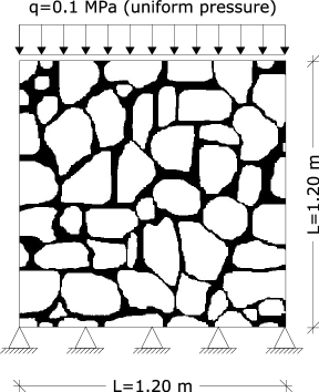
Figure 5. Scheme of an illustrative example

The finite element model of the example problem was based on a regular discretization of the domain using $24\times 24$ square bilinear elements with four integration points. Note that such a resolution corresponds to the element edge approximately equal to a half of the geometrical correlation length, which is fully consistent with general rules discussed in Sections 3–5.

The results presented for the KLE-based solver were derived from $n=1,000$ simulations. For simplicity, only the Young modulus $E$ considered in the form of a random field (see Figure 6 for an illustration), whereas the Poisson ratio was set to a deterministic value determined from the Voigt estimate of the homogenized stiffness matrix

$${\boldsymbol{\mu}}_{{\boldsymbol{C}}}=c^{(m)}{\boldsymbol{C}}^{(m)}+c^{(s)}{\boldsymbol{C}}^{(s)}.$$ (50)

Finally, based on a systematic one-dimensional study of the HS approach presented in [38], the element-wise constant discretization of the phase polarization stresses with four-point integration scheme was adopted to ensure sufficient resolution of the spatial statistics. Additional implementation-related details can be found in [24].

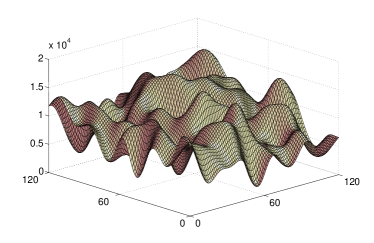
(a)

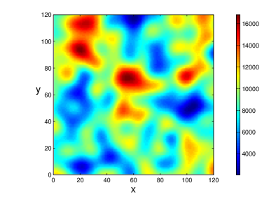
(b)

Figure 6. Realization of Gaussian random field of Young’s modulus

Before presenting the comparison of individual approaches, we concentrate first on the effect of reference media on the HS-based predictions. To this end, the expected values of nodal displacements are plotted in Figure 7 for several representative choices of ${\boldsymbol{C}}_{0}$. In particular, owing to the dominant fraction of the stiffer phase ($c^{(s)}\doteq 67\%$) in the considered structure, the lower energetic bound can be expected to be substantially closer to the “true” statistics than the corresponding upper bound, which in the current case seems to be too inaccurate for practical use. Additional estimates can be generated by the Voigt-type choice (50) or by setting the reference medium to the arithmetic average of properties of individual constituents, the value commonly adopted in the polarization-based numerical method due to Moulinec and Suquet [31]. As expected, the response corresponding to such choices is comparable to the lower bound and will be used in the sequel for the comparison with the candidate approaches.

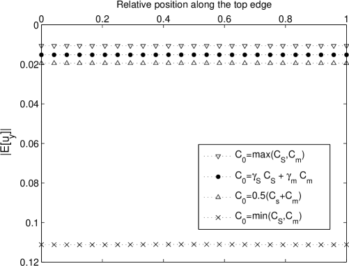
Figure 7. Expected value of nodal displacements via HS-based FE analysis

The basic statistics of nodal displacements, as predicted by different methods, are mutually compared in Figure 8. In addition, we present the confidence bounds in the form ${\boldsymbol{\mu}}_{{\boldsymbol{u}}_{h}}({\boldsymbol{x}})\pm{\boldsymbol{\sigma}}_{{\boldsymbol{u}}_{h}}({\boldsymbol{x}})$, determined on the basis of the second-order statistics for the improved perturbation method (24) or KLE (33). In general, it can be seen that the perturbative method leads to a substantially wider confidence interval when compared to the Monte-Carlo simulation approach, in spite of a moderate number of simulations used by KLE solver to estimate the overall statistics. For both methods, the confidence intervals remain bounded from above by the corresponding HS value. Moreover, for appropriate choices of the reference stiffness matrix, the HS method recovers the predictions provided by the alternative approaches. For the current setting, selecting ${\boldsymbol{C}}_{0}$ according to the rule of mixtures yields the displacement values almost identical to that of the KLE solver, whereas the response related to the arithmetic average well approximates the improved perturbation result. These results provide just another highlight of the importance of a proper choice of the reference media in the HS-based schemes, see e.g. [8, 38] for further discussion.

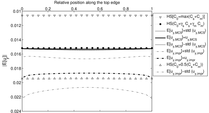
Figure 8. Basic statistics of nodal displacements on the top of the panel

The final comment concerns the computational complexity of individual approaches. It can be stated that the cost of the improved perturbation method and the HS-based solver is roughly comparable, whereas the KLE approach leads to an approximately three-fold increase in the simulation time. Higher cost of the latter method can be attributed to a large number of terms appearing in the expansion (29); the computational cost, however, is compensated by generality of the Monte-Carlo framework and can be further reduced by parallelization of the problem.

7. Conclusions and future work

In this contribution, the applicability of three distinct approaches to mesostructure-based random field simulation of irregular historic masonry was investigated. The numerical results obtained for a finite-size elastic panel allow us to reach the following conclusions:

• The elements of quantification of random spatial statistics can be efficiently used to construct realistic first- and second-order statistics of stationary random fields.

• The improved perturbation method utilizes the second-order statistics when determining the mean response of the system, which generally leads to narrower estimates when compared with the basic method, e.g. [24, Chapter 5]. In the current case, however, the uncertainty in the obtained statistics is higher than for the KLE algorithm, mainly due to a relatively high contrast of phase stiffnesses.

• The Karhunen-Loève series representation coupled with the Monte Carlo approach provides an interesting alternative to the perturbation-based method, even at increased computational cost. When applied to realistic structures, however, a large number of terms seems to be necessary to capture the available covariance information. Moreover, the validity of the Gaussian assumption needs to be critically assessed.

• The Hashin-Shtrikman approach takes advantage of the specific form of the random field and therefore optimally utilizes the available information. The overall response is in this case, however, highly dependent on the choice of the reference medium, for which there is no general rule.

Even though the results of this pilot study have provided valuable insights into the pros and cons of individual methods, they do not allow for directly quantifying the accuracy of individual methods as the reference solution is not available. Similarly to a recent study [38], such a comparison can be based on a synthetic mesostructural model such the one proposed by Spence at al. [39]. This particular topic enjoys our current interest and will be reported separately.

References

- [1] A. Anthoine. Derivation of the in-plane elastic characteristics of masonry through homogenization theory. International Journal of Solids and Structures, 32(2):137–163, 1995.
- [2] I. Babuška, R. Tempone, and G. E. Zouraris. Solving elliptic boundary value problems with uncertain coefficients by the finite element method: the stochastic formulation. Computer Methods in Applied Mechanics and Engineering, 194(12–16):1251–1294, 2005.
- [3] A. Bensoussan, J.L. Lions, and G. Papanicolaou. Asymptotic analysis for periodic structures. Studies in Mathematics and its Applications. North-Holland, Amsterdam, 1978.
- [4] Z. Bittnar and J. Šejnoha. Numerical methods in structural mechanics. ASCE Press and Thomas Telford, Ltd., New York and London, 1996.
- [5] V. Buryachenko. Micromechanics of heterogeneous materials. Springer Verlag, New York, NY, USA, 2007.
- [6] D. C. Charmpis, G. I. Schueller, and M. F. Pellissetti. The need for linking micromechanics of materials with stochastic finite elements: A challenge for materials science. Computational Materials Science, 41(1):27–37, 2007.
- [7] F. Cluni and V. Gusella. Homogenization of non-periodic masonry structures. International Journal of Solids and Structures, 41(7):1911–1923, 2004.
- [8] G. J. Dvorak and M. V. Srinivas. New estimates of overall properties of heterogeneous solids. Journal of the Mechanics and Physics of Solids, 47(4):899–920, 1999.
- [9] I. Elishakoff, Y. J. Ren, and M. Shinozuka. Improved finite element method for stochastic problems. Chaos, Solitons & Fractals, 5(5):833–846, 1995.
- [10] G. Falsone and M. Lombardo. Stochastic representation of the mechanical properties of irregular masonry structures. International Journal of Solids and Structures, 44(25–26):8600–8612, 2007.
- [11] J. Gajdošík, J. Zeman, and M. Šejnoha. Qualitative analysis of fiber composite microstructure: Influence of boundary conditions. Probabilistic Engineering Mechanics, 21(4):317–329, 2006.
- [12] R. Ghanem and P. D. Spanos. Spectral stochaststic finite element formulation for reability analysis. Journal of Engineering Mechanics ASCE, 117(10):2351–2372, 1991.
- [13] R. Ghanem and P. D. Spanos. Stochastic finite elements: A spectral approach. Dover Publications, Mineola, New York, second revised edition, 2003.
- [14] V. Gusella and F. Cluni. Random field and homogenization for masonry with nonperiodic microstructure. Journal of Mechanics of Materials and Structures, 1(2):357–386, 2006.
- [15] Z. Hashin and S. Shtrikman. On some variational principles in anisotropic and nonhomogeneous elasticity. Journal of the Mechanics and Physics of Solids, 10:335–342, 1962.
- [16] S. P. Huang, S. T. Quek, and K. K. Phoon. Convergence study of truncated Karhunen-Loève expansion for simulation of stochastic process. International Journal for Numerical Methods in Engineering, 52(9):1029–1043, 2001.
- [17] C. Huet. Application of variational concepts to size effects in elastic heterogeneous bodies. Journal of the Mechanics and Physics of Solids, 38(6):813–841, 1990.
- [18] M. Jardak and R. G. Ghanem. Spectral stochastic homogenization of divergence-type PDEs. Computer Methods in Applied Mechanics and Engineering, 193(6-8):429–447, 2004.
- [19] V. V. Jikov, S. M. Kozlov, and O. A. Oleinik. Homogenization of Differential Operators and Integral Functionals. Springer-Verlag, 1994.
- [20] M. Kamiński. Homogenization in elastic random media. Computer Assisted Mechanics and Engineering Sciences, 3(1):9–21, 1996.
- [21] M. Kamiński. Computational Mechanics of Composite Materials: Sensitivity, Randomness and Multiscale Behaviour. Springer Verlag, London, 2004.
- [22] M. Kamiński and M. Kleiber. Perturbation based stochastic finite element method for homogenization of two-phase elastic composites. Computers & Structures, 78(6):811–826, 2000.
- [23] U. Kowalsky, T. Zumendorf, and D. Dinkler. Random fluctuations of material behaviour in FE-damage analysis. Computational Materials Science, 39(1):8–16, 2007.
- [24] M. Lombardo. Random field models and stochastic analysis of irregular masonry structures. PhD thesis, Univesità degli Studi di Messina, Facoltà di Ingegneira, Dipartmento di Ingegneira Civile, Messina, Italy, 2008.
- [25] P.B. Lourenco, G. Milan, A. Tralli, and Zucchini A. Analysis of masonry structures: Review of and recent trends in homogenization techniques. Canadian Journal of Civil Engineering, 34(11):1443–1457, 2007.
- [26] R. Luciano and J. R. Willis. FE analysis of stress and strain fields in finite random composite bodies. Journal of the Mechanics and Physics of Solids, 53(7):1505–1522, 2005.
- [27] R. Luciano and J.R. Willis. Hashin-Shtrikman based FE analysis of the elastic behaviour of finite random composite bodies. International Journal of Fracture, 137(1–4):261–273, 2006.
- [28] T.J. Massart, R.H.J. Peerlings, and M.G.D. Geers. An enhanced multi-scale approach for masonry wall computations with localization of damage. International Journal for Numerical Methods in Engineering, 69(5):1022–1059, 2007.
- [29] H.G. Matthies, C.E. Brenner, C. G. Bucher, and C. G. Soares. Uncertainties in probabilistic numerical analysis of structures and solids: Stochastic finite elements. Structural Safety, 19(3):283–336, 1997.
- [30] H.G. Matthies and A. Keese. Galerkin methods for linear and nonlinear elliptic stochastic partial differential equations. Computer Methods in Applied Mechanics and Engineering, 194(12–16):1295–1331, 2005.
- [31] H. Moulinec and P. Suquet. A numerical method for computing the overall response of nonlinear composites with complex microstructure. Computer Methods in Applied Mechanics and Engineering, 157(1–2):69–94, 1998.
- [32] G. L. Povirk. Incorporation of microstructural information into models of two-phase materials. Acta Metallurgica et Materialia, 43(8):3199–3206, 1995.
- [33] P. Procházka and J. Šejnoha. Extended Hashin-Shtrikman variational principles. Applications of Mathematics, 49(4):357–372, 2004.
- [34] K. Sab. On the homogenization and the simulation of random materials. European Journal of Mechanics A-Solids, 11(5):585–607, 1992.
- [35] S. Sakata, F. Ashida, T. Kojima, and M. Zako. Three-dimensional stochastic analysis using a perturbation-based homogenization method for elastic properties of composite material considering microscopic uncertainty. International Journal of Solids and Structures, 45(3–4):894–907, 2008.
- [36] S. Sakata, F. Ashida, and M. Zako. Kriging-based approximate stochastic homogenization analysis for composite materials. Computer Methods in Applied Mechanics and Engineering, 197(21–24):1953–1964, 2008.
- [37] C.A. Schenk and G.I. Schuëller. Buckling analysis of cylindrical shells with random geometric imperfections. International Journal of Non-Linear Mechanics, 38(7):1119–1132, 2003.
- [38] Z. Sharif-Khodaei and J. Zeman. Microstructure-based modeling of elastic functionally graded materials: One dimensional case. Journal of Mechanics of Materials and Structures, 2008. accepted for publication, e-print: arXiv/0802.0511.
- [39] S. M. Spence, M. Gioffré, and M. D. Grigoriu. Probabilistic models and simulation of irregular masonry walls. Journal of Engineering Mechanics ASCE, 134(9):750–762, 2008.
-
[40]
B. Sudret and A. Der Kiureghian.
Stochastic finite element methods and reliability: A state of the
art report.
Technical Report UCB/SEMM-2000/08, Univesity of California, Berkley,
2000.
Available at
http://nisee.berkeley.edu/documents/SEMM/SEMM-2000-08.pdf []. - [41] S. Torquato. Random heterogeneous materials: Microstructure and macroscopic properties. Springer-Verlag, 2002.
- [42] E. Vanmarke. Random fields: Analysis and Synthesis. MIT Press, 1998.
-
[43]
M. Šejnoha, J. Zeman, and J. Novák.
Homogenization of random masonry structures - Comparison of
numerical methods.
In EM 2004 - 17th ASCE Engineering Mechanics Division
Conference, page 8 pp., Newark, US, 2004. University of Delaware.
http://chinacat.coastal.udel.edu/~kirby/EM2004/paperfinal/48.pdf []. - [44] J. R. Willis. Bounds and self-consistent estimates for the overall properties of anisotropic composites. Journal of the Mechanics and Physics of Solids, 25:185–202, 1977.
- [45] F. X. Xu. A multiscale stochastic finite element method on elliptic problems involving uncertainties. Computer Methods in Applied Mechanics and Engineering, 196(25–28):2723–2736, 2007.
- [46] F. X. Xu and L. Graham-Brady. A stochastic computational method for evaluation of global and local behavior of random elastic media. Computer Methods in Applied Mechanics and Engineering, 194(42–44):4362–4385, 2005.
- [47] F. X. Xu and L. Graham-Brady. Computational stochastic homogenization of random media elliptic problems using Fourier Galerkin method. Finite Elements in Analysis and Design, 42(7):613–622, 2006.
- [48] J. Zeman and M. Šejnoha. From random microstructures to representative volume elements. Modelling and Simulation in Materials Science and Engineering, 15(4):S325–S335, 2007.
- [49] J. Zhang and B. Hellingwood. Orthogonal series expansion of random fields in reliability analysis. Journal of Engineering Mechanics ASCE, 120(12):2660–2677, 1994.