The infinite partition of a line segment and multifractal objects

Abstract

We report an algorithm for the partition of a line segment according to a given ratio $\nu$. At each step the length distribution among sets of the partition follows a binomial distribution. We call $k$-set to the set of elements with the same length at the step $n$. The total number of elements is $2^{n}$ and the number of elements in a same $k$-set is $C_{n}^{k}$. In the limit of an infinite partion this object become a multifractal where each $k$-set originate a fractal. We find the fractal spectrum $D_{k}$ and calculate where is its maximum. Finally we find the values of $D_{k}$ for the limits $k/n\rightarrow 0$ and $1$.

keywords: multifractal, binomial distribution, partition of a segment, spectrum of fractal dimensions.

1 Introduction

Multifractals have been largely employed in the characterization of time series. This tool have been successfully applied in many different areas as economics [1], meteorology [2], geology [3], or biomedical [4]. Several algorithms have been used to find the multifractal spectrum of the time-series, for instance, wavelet analysis [5] and DFA (Detrended fluctuation analysis) [6]. However, despite the large use of multifractals as a time-series analysis technique there is no simple geometrical examples of multifractal sets.

Some years ago it was introduced a multifractal partition of the unit square [7]. This mathematical object was originally developed to model multifractal heterogeneity in oil reservoirs and to study percolation on complex lattices. Afterwards, a generalization of this object to random partitions was performed to improve the model [8, 9]. In this work we explore the unidimensional version of this model. Indeed, the multifractal partition of the square, cube or hypercube are, in essence, derived from a multifractal partition of a line segment.

Cantor sets, Peano curves or Sierpinski models are very useful subjects to grasp the fundamentals of fractals. On the other side, the study of multifractal sets lack simple geometrical examples. This paper intend to fulfill this vacancy in the literature. The work is organized as follows. In section $2$ we introduce the partition of a line segment that produces a multifractal set. We focus our attention on the case of a constant cutting ratio $\nu$. The binomial distribution naturally arises in the construction of the partition algorithm. In section $3$ we analytically derive the multifractal spectrum $D_{k}$ of the partition and find its limit cases $k/n\rightarrow 0$ and $1$. We use a method similar to the boxcounting algorithm. Finally in section $4$ we give our final remarks.

2 The partition of a line segment according to a ratio

In this section we introduce a partition of a line segment. We expose the method of construction of the partition as a recursive algorithm. We call the sets at step $n$ as father sets respect to son-sets at step $n+1$. Each father set always give origin to two son sets. The sum of lengths of the son sets is equal to the length of the father set, that means, the dynamic rule of the algorithm is length preserving. At each step of the algorithm we use a ratio $\nu$ to perform the partition of the father sets. In the next paragraphs we will detail the initial steps of the algorithm, but the multifractal, that shall be shown in the next section, is properly defined in the limit of $n$ going to infinity.

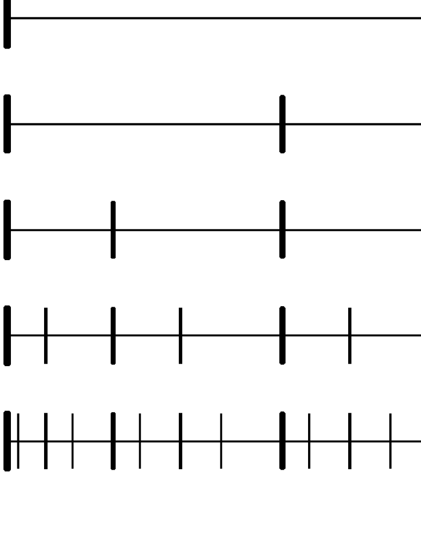
Figure 1: A pictorial representation of the five initial steps of the partition of a line segment for a constant ratio. The partitions are indicated by vertical thick marks. For sake of clarity, the thick marks of the father-sets are always thicker than the son-sets. At step $n$ the number of sets is $N_{n}=2^{n}$. The elements with the same length form a $k$-set, there are $C_{n}^{k}$ elements in a $k$-set. The length distribution among sets obeys a binomial rule.

In figure 1 we show a representation of the five initial steps in the construction of our partition. The step $n=0$ corresponds to the segment of length $L$ itself. At step $n=1$ the segment is partitioned into two pieces of length $\nu L$ and $(1-\nu)L$. At step $n=2$ the two pieces are each one partitioned into two new sets giving origin to $4$ sets and so on. In table 1 we show the iteration step $n$, the number of sets for each step $N_{n}=2^{n}$ and the partition length (as a fraction of $L$) inside each step. We notice that the length distribution is trivially done by a binomial rule, that means, the partition gives raise, at step $n$, to a binomial length distribution:

$$L=\sum_{k=0}^{n}C_{n}^{k}\nu^{k}(1-\nu)^{(1-k)}L$$ (1)

Table 1: The main quantities of the algorithm of the partition of a segment line according to a ratio $\nu$. The iteration step $n$, the total number of sets at each step $N_{n}$, the full length partition as a fraction of $L$.

$n$	$N_{n}$	Partition length (in unities of $L$)
$0$	1	1
$1$	2	$\nu$ + $(1-\nu)$
$2$	4	$\nu^{2}+2\nu(1-\nu)+(1-\nu)^{2}$
$3$	8	$\nu^{3}+3\nu^{2}(1-\nu)+3\nu(1-\nu)^{2}+(1-\nu)^{3}$
		…
$n$	$2^{n}$	$\sum_{k=0}^{n}C_{n}^{k}\nu^{k}(1-\nu)^{(1-k)}$

We remark some differences between the exposed process and the algorithm construction of Cantor set and Koch curve [11]. Initially the cited fractals do not conserve length along the dynamic formation, the measure divergence in these sets is originated in the algorithm process itself, the Cantor set subtracts subsets and the Koch adds subsets at each step. In addition, in these fractal models all sets, at the same step of their generating algorithm, have the same length. By that reason these models produce monofractal sets.

We call $k$-sets the set of all elements, at the step $n$, that has the same length $\nu^{k}(1-\nu)^{(1-k)}L$. By construction there are $C_{n}^{k}$ elements in a $k$-set. In the next section, for the limit of $n\rightarrow\infty$ we will determine the fractal dimension of each $k$-set and characterize the set of all $k$-set as a multifractal object.

To find the length partition of a line segment in the case of variable $\nu$ we proceed as follows. Consider that $\nu_{i}$ is present $n_{i}$ times at the partition and that at step $n$ we have $n=n_{1}+n_{2}+...+n_{l}$. In this case the length distribution is done by:

$$L=\frac{n!}{n_{1}!n_{2}!...n_{l}!}\nu_{1}^{n_{1}}\nu_{2}^{n_{2}}...\nu_{l}^{n_{l}}L$$ (2)

In figure 1 we assume a fixed rule in the partition. Each time a father set is cut into two new pieces the largest son set is always situated at the right position. We notice that this is an arbitrary choice that will not change the length distribution of the object. On the other side, the topology of the partition (a subject that we do not consider in this paper) will change since the neighborhood properties will change. We cite that the bidimensional version of the multifractal has a topological treatment [10] that can not be easily extended to the unidimensional object. In fact, the topology of a line segment is sort of trivial since each open set in the segment has always two neighbours. In the cited work [10] we report that the bidimensional multifractal version of the object we work in this paper has a power-law distribution of neighbours.

3 The multifractal spectrum

In this section we estimate the fractal dimension for each $k$-set that results from the partition of a segment. We calculate the fractal dimension of each $k$-set, $D_{k}$, with help of the definition:

$$D_{k}=lim_{\epsilon\rightarrow 0}\frac{log(N(k))}{log(1/\epsilon)}$$ (3)

In this definition $N(k)$ is the number of open balls, of size $\epsilon$, necessary to cover a given $k$-set.

In order to use (3) we generate a proper coverage of the segment $L$. To create an adequate coverage of the partition we take at step one $L=s+r$ for $r,s$ integers. Therefore $\nu$ is a rational number $\nu=r/(s+r)$ (we take $r<s$). In addition, at each step $n$ the size of the segment is $L=(s+r)^{n}$ and the size of the open balls used to cover the $k$-sets is:

$$\epsilon_{n}=\frac{1}{L}=\frac{1}{(s+r)^{n}}$$

In this way, $N(k)$, the total length of each $k$-set is $C_{n}^{k}r^{k}s^{(n-k)}$ and as a result $D_{k}$ is done by:

$$D_{k}=lim_{n\rightarrow\infty}\frac{log(C_{n}^{k}\>r^{k}\>s^{(n-k)})}{log((r+s)^{n})}$$ (4)

In figure 2 we computationally test the finite size effect over the multifractal spectrum (4). We use as a case study $r=1$ and $s=2$ and as a consequence $\nu=\frac{1}{2+1}=\frac{1}{3}$. In the simulations we take $n=10,20,40$, $80$ and $160$ to follow the convergence of the spectrum. In this figure we plot $k/n$ in the horizontal axis to compare the results of several $n$. We observe in the data that in the limit of large $n$ the spectrum seems to touch the line $D=1$ which suggests that the $k$-set of largest dimension is dense in the line.

It is interesting to estimate $D_{k}$ in the limits of $k$ going to $0$ and $n$. Using equation (4) we calculate $D_{k}$ for $k\rightarrow 0$:

$$D_{k}=\frac{log(C_{n}^{0}\>r^{0}\>s^{(n-0)})}{log((r+s)^{n})}=\frac{n\>log(1s)}{n\>log(r+s)}=\frac{log(s)}{log(s+r)}.$$

Summarizing, we have:

$$k\rightarrow 0\hskip 28.45274ptD_{0}=\frac{log(s)}{log(r+s)}.$$ (5)

In a similar way we estimate:

$$k\rightarrow n\hskip 28.45274ptD_{n}=\frac{log(r)}{log(r+s)}.$$ (6)

We use the notation $k\rightarrow 0$ instead of $k=0$ because he multifractal is only defined in the limit of $n\rightarrow\infty$, and therefore $k=0$ is in fact an accumulation point. It is worth to note that in the limit of $k\rightarrow 0$ or $k\rightarrow\infty$ the fractal dimension is not necessarily $0$. One could think that $D_{k}=0$ for $k=0$ because the multifractal of the corresponding $k$-set for $k=0$ is composed by just one point and the dimension of a single point is zero. This argument is not valid because the multifractal is only properly defined in the limit of $n\rightarrow\infty$, where the variable $k$ is not discrete, but continuous.

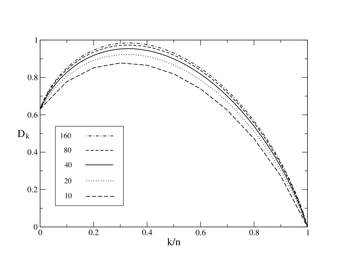
Figure 2: The multifractal spectrum $D_{k}$ versus $k/n$. The number of steps in the algorithm is $n=10,20,40,80$ and $160$ as indicated in the figure. We use $r=1$ and $s=2$ as a case study.

We show the spectrum of fractal dimension for several ratios $\nu$ in figure 3. We display in this plot the spectrum $D_{k}$ versus $k/n$ for some $s$ and $r$ as indicated in the figure. In this estimation we use $n=100$. The relations (5) (6) are verified in the curves of the figure.

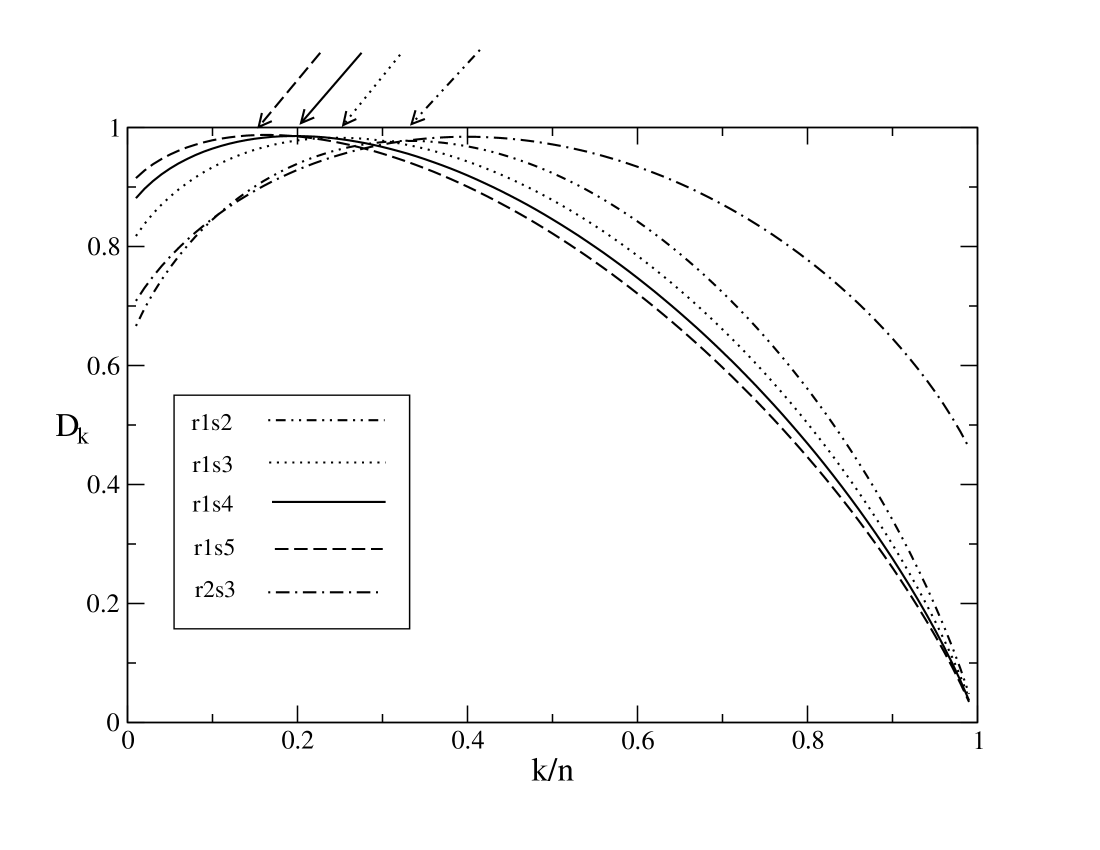
Figure 3: The multifractal spectrum $D_{k}$ for several ratio partitions as indicated in the figure. The maximum of each curve is evaluated in the text and indicated in the figure by arrows at the top of the figure. The limits of $k/n\rightarrow 0$ and $1$ are analytically determined in the text.

We find the maximum of $D_{k}$ for any $\nu$ using the property of the maximum of the binomial distribution [12]. In this way the maximum of $D_{k}$ is at $\nu n$ or $\frac{r}{s+r}n$. To compare this result with the maximum of curves in figure 3 we use the normalization $k/n$ and the maximum is at $\nu$. We check in the figure, for instance, that the maxima for the cases $r=1$ and $s=2,3,4$ and $5$ are at positions $\nu=\frac{1}{3},\frac{1}{4},\frac{1}{5}$ and $\frac{1}{6}$ respectively. These values are indicated by successive arrows in the plot.

The degenerate case $r=s=1$ corresponds to the standard partition of a segment which generates the unidimensional lattice. In this limit all elements of the partition have the same size. Following this rule we cover the line segment with $2^{n}$ equal elements of length $\epsilon=1/2^{n}$ and the dimension of the object is not a fractal, indeed $\frac{log2^{n}}{log2^{n}}=1$ In this case there is just one $k$-set that trivially have the same dimension of the line segment itself.

4 Final remarks

In this work we introduce an object that arises from an infinite partition of a line segment. We present the construction algorithm of the object as a recursive sequence. In the case of a constant partition ratio $\nu$ the length distribution of its elements, at step $n$ of the algorithm, follows a binomial distribution. At step $n$, the partition is formed by $2^{n}$ sets grouped in $(n+1)$ $k$-sets, that means, sets whose elements share the same length $\nu^{k}(1-\nu)^{(1-k)}$. In the limit of $n\rightarrow\infty$ each $k$-set is a monofractal set. The multifractal set is composed by the totality of infinite monofractal sets. In addition we find the fractal spectrum $D_{k}$ and estimate where is its maximum. Finally we find the values of $D_{k}$ for the limits $k/n\rightarrow 0$ and $1$.

In this work we adapted to a line segment an algorithm of generation of multifractal objects that was initially defined on a square. The route from two dimensions to one dimension is a challenge. At one side we loose the attractive idea of modeling bidimensional geological formations. Otherwise, once we go to an unidimensional version of the problem some points became more clear: the generalization of this object to any dimension, its formation algorithm and the spectrum of fractal dimensions.

We think we have also attained our aims by showing to a general reader an illustrative ans simple geometrical multifractal set. However, some questions about this multifractal set remain open. Is the largest set of the multifractal dense in the line? The simulations indicate a positive answer, but we lack a rigorous proof of that. Following equation (2), is there a simple spectrum of dimensions for the case of non constant partition? The answer seems positive if we could define appropriate $k$-sets. A more general question would be: if the set of ratios $\nu_{i}$ in equation (2) follows a normal distribution, what will be the resulting multifractal? We conjecture that this new object would be usefull as a benchmark to compare with empirical multifractals.

Acknowledgments

We thank the financial support from CNPq (Conselho Nacional de Pesquisa).

References

- [1] Z. Eisler and J. Kertésza, Physica A, 343 603 (2004).
- [2] G. Calenda, E. Gorgucci, F. Napolitano, A. Novella, and E. Volpi, Adv. Geosci., 2 293 (2005).
- [3] L. Telesca, G. Colangelo, V. Lapenna, and M. Macchiato, Chaos, Solitons and Fractals, 18 385 (2003).
- [4] A. N. Pavlov, A. R. Ziganshin, O. A. Klimova, Chaos, Solitons and Fractals, 24 57 (2005).
- [5] A. Arneodo, G. Grasseau and M. Holschneider, Physical Review Letters 61 2281 (1988).
- [6] J. W. Kantelhardt, S. A. Zschiegner, E. Koscielny-Bunde, S. Havlin, A. Bunde, and H. E. Stanley, Physica A, 316 87 (2002).
- [7] G. Corso, J. E. Freitas, L. S. Lucena, and R. F. Soares, Physical Review E, 69 066135 (2004).
- [8] M. G. Pereira, G. Corso, L. S. Lucena, J. E. Freitas, International Journal of Modern Physics C, 16 317 (2005).
- [9] M. G. Pereira, G. Corso, L. S. Lucena, J. E. Freitas, Chaos Solitons and Fractals, 23 1105 (2005).
- [10] G. Corso, J. E. Freitas, L. S. Lucena, Physica A 342, 214 (2004).
- [11] Michael Barsnley, Fractals Everywhere, Academic Press, Boston, (1988).
- [12] Paul L. Meyer, Introductory Probability and Statistical Applications, Addison-Wesley, New York, (1965).