Quasiparticle excitations and dynamic susceptibilities in the BCS-BEC crossover

Abstract

We study dynamic ground state properties in the crossover from weak (BCS) to strong coupling (BEC) superfluidity. Our approach is based on the attractive Hubbard model which is analyzed by the dynamical mean field theory (DMFT) combined with the numerical renormalization group (NRG). We present an extension of the NRG method for effective impurity models to self-consistent calculations with superconducting symmetry breaking. In the one particle spectra we show quantitatively how the Bogoliubov quasiparticles at weak coupling become suppressed at intermediate coupling. We also present results for the spin and charge gap. The extension of the NRG method to self-consistent superconducting solutions opens the possibility to study a range of other important applications.

Introduction -

There has been a resurgence of interest into the nature of the crossover from the weak coupling Bardeen, Cooper, and Schrieffer (1957) (BCS) superfluidity to the Bose Einstein condensation (BEC) of preformed pairs, due to its recent experimental realization for ultracold atoms in an optical trapGreiner et al. (2003); Zwierlein et al. (2004, 2005); Bloch et al. (2008). In the ultracold atom experiments, the interactions between the fermionic atoms in the trap can be tuned by a Feshbach resonance permitting an unprecedented control of the parameters, so that theoretical predictions may now be put to an experimental test. Above the transition temperature the two limiting cases, BCS superconductivity and BEC, correspond to quite different physical situations. The weak coupling BCS theory describes a fermionic system with Cooper instability, whereas the strong coupling BEC limit is a system of strongly bound fermion pairs, which obey Bose statistics. The theoretical understanding which has been developed over the years is that the properties, such as the order parameter $\Delta_{\rm sc}$ and the transition temperature $T_{c}$ to the superfluid state, are connected by a smooth crossover, and approximate interpolation schemes between these limits have been devised Eagles (1969); Leggett (1980); Nozières and Schmitt-Rink (1985); Randeria (1995).

There is experimental evidence that the BCS-BEC crossover has also relevance for strong coupling and high temperature superconductors. These superconductors display properties, it has been claimed Micnas et al. (1990); Toschi et al. (2005a); Chen et al. (2006), that can be understood in terms of local pairs, preformed above the transition temperature $T_{c}$, in contrast to the BCS picture, where the pairs no longer exist above $T_{c}$.

As more experimental techniques, such as pairing gap spectroscopy Chin et al. (2004); Greiner et al. (2005), are being developed to probe this crossover, more detailed theoretical predictions are required. In particular the dynamic response functions have received little theoretical attention, and it is the predictions for these quantities through the crossover that will be the focus of the present paper.

Here, we use the attractive Hubbard model Micnas et al. (1990) to study the crossover. In order to investigate the full crossover regime from weak to strong coupling a reliable non-perturbative method is needed. We employ the dynamical mean field theory (DMFT), together with the numerical renormalization group (NRG) to treat the effective impurity problem. DMFT studies, which are appropriate for the three and higher dimensional case, for the attractive Hubbard model with other methods for the effective impurity problem have been carried out in the normal phaseKeller et al. (2001); Capone et al. (2002), and more recently in the symmetry-broken phaseGarg et al. (2005); Toschi et al. (2005b, a). But spectral properties have not been calculated and analyzed in detail there. There have been calculations of the dynamic response functions for the two dimensional model, for example with quantum Monte Carlo Singer et al. (1996) or recent work using the cellular DMFT Kyung et al. (2006). Our results based on the DMFT are not expected to be directly applicable to this low dimensional case, but a comparison can be of interest to see if there are common trends.

Our method to study the effective impurity problem, the NRG, is a non-perturbative method originally devised by WilsonWilson (1975) to analyze the many body problem in the Kondo model and Anderson impurity model (AIM). In this approach the high energy degrees of freedom are eliminated numerically to find a an effective low energy theory, and its early application contributed vitally to the quantitative understanding of the Kondo problem Hewson (1993). The method was developed further in the 1990s, when it was extended to the calculation of spectral functions Sakai et al. (1989); Costi et al. (1994). After the advent of the DMFTGeorges et al. (1996) it was realized then that it could be used for self-consistent solutions of the effective impurity problem Bulla et al. (1997). The calculation of spectral functions was improved further by approaches based on the density matrix Hofstetter (2000) and the complete basis set proposed by Anders and Schiller Anders and Schiller (2005); Peters et al. (2006); Weichselbaum and von Delft (2007). Our approach uses this latest full density matrix scheme to calculate reliable spectral functions. The NRG method and its applications are comprehensively reviewed by Bulla et al. Bulla et al. (2008).

In the original theory and in many of the applications one deals with a metallic system, where the NRG inherent logarithmic discretization and the descent to low energies gives the accurate low energy properties. However, the method has also given reliable results in situations with a gap in the spectrum. Examples include the Mott transition Bulla (1999) or antiferromagnetic solutions Zitzler et al. (2002); Bauer and Hewson (2007) in the repulsive Hubbard model in the DMFT-NRG framework. There is also an extensive amount of work for situations where the bath of the impurity model is a mean field BCS superconductor with given energy gap Satori et al. (1992); Sakai et al. (1993); Yoshioka and Ohashi (2000); Choi et al. (2004); Oguri et al. (2004); Bauer et al. (2007); Hecht et al. (2008). The NRG parameters for the bath in this case are fixed and can be determined by a straightforward generalization of the original NRG approach. Here, we present the extension of the method to calculations where the parameters describing the superconducting bath have to be determined self-consistently, which is a requirement of the DMFT approach, where the impurity is an effective one and plays an auxiliary role. This opens the possibility to study a number of interesting non-perturbative problems involving superconductivity in a well controlled framework.

Formalism -

Our study is based on the attractive Hubbard model Micnas et al. (1990),

$$H=-\sum_{i,j,\sigma}(t_{ij}c^{\dagger}_{i,\sigma}c_{j,\sigma}+\mathrm{h.c.})-\mu\sum_{i\sigma}n_{i\sigma}-U\sum_{i}n_{i,\uparrow}n_{i,\downarrow},$$ (1)

with the chemical potential $\mu$, the interaction strength $U>0$ and the hopping parameters $t_{ij}$. $c^{\dagger}_{i,\sigma}$ creates a fermion at site $i$ with spin $\sigma$, and $n_{i,\sigma}=c^{\dagger}_{i,\sigma}c_{i,\sigma}$. For the DMFT calculation we employ the Anderson impurity model in a superconducting medium as the effective impurity model,

$$H_{\mathrm{And}} = H_{\rm imp}+\sum_{{\bm{k}},{\sigma}}\varepsilon_{{\bm{k}}}c^{\dagger}_{{\bm{k}},\sigma}c_{{\bm{k}},\sigma}+\sum_{{\bm{k}},{\sigma}}V_{{\bm{k}}}(c^{\dagger}_{{\bm{k}},\sigma}{d}_{\sigma}+\mathrm{h.c.})$$ (2)

$$-\sum_{{\bm{k}}}\Delta_{{\bm{k}}}[c^{\dagger}_{{\bm{k}},\uparrow}c^{\dagger}_{-{\bm{k}},\downarrow}+c_{-{\bm{k}},\downarrow}c_{{\bm{k}},\uparrow}],$$

where $H_{\rm imp}=\sum_{\sigma}\varepsilon_{d}n_{d,\sigma}-Un_{d,\uparrow}n_{d,\downarrow}$ and $d_{\sigma}$ is the fermionic operator at the impurity site. $\varepsilon_{{\bm{k}}}$, $V_{{\bm{k}}}$ and $\Delta_{{\bm{k}}}$ are parameters of the medium. The non-interacting Green’s function matrix at $T=0$ has the form,

$$\underline{G}_{0}(\omega)^{-1}=\omega\mathbbm{1}_{2}-\varepsilon_{d}\tau_{3}-\underline{K}(\omega).$$ (3)

$\underline{K}(\omega)$ is the generalized matrix hybridization for the medium, with diagonal part

$$K_{11}(\omega)=\frac{1}{N}\sum_{{\bm{k}}}V_{{\bm{k}}}^{2}\frac{\omega+\varepsilon_{{\bm{k}}}}{\omega^{2}-(\varepsilon_{{\bm{k}}}^{2}+\Delta_{{\bm{k}}}^{2})}$$ (4)

and offdiagonal part,

$$K_{21}(\omega)=\frac{1}{N}\sum_{{\bm{k}}}V_{{\bm{k}}}^{2}\frac{\Delta_{{\bm{k}}}}{\omega^{2}-(\varepsilon_{{\bm{k}}}^{2}+\Delta_{{\bm{k}}}^{2})}.$$ (5)

In the DMFT with superconducting symmetry breaking the effective Weiss field is a $2\times 2$ matrix $\underline{{\cal G}}_{0}^{-1}(t)$Georges et al. (1996). The DMFT self-consistency equation in this case also is a matrix equation,

$$\underline{{\cal G}}_{0}^{-1}(\omega)=\underline{G}(\omega)^{-1}+\underline{\Sigma}(\omega),$$ (6)

with the ${\bm{k}}$-independent self-energy $\underline{\Sigma}(\omega)$ and the local lattice Green’s function $\underline{G}(\omega)$. We identify as usual $\underline{G}_{0}(\omega)=\underline{{\cal G}}_{0}(\omega)$. Having calculated the local Green’s function $\underline{G}$ and the self-energy $\underline{\Sigma}(\omega)$, the self-consistency equation (6) determines the new Weiss field and medium as input for the effective impurity problem. Once $K_{11}(\omega)$ and $K_{21}(\omega)$ are given by (6), the problem is to calculate the effective impurity model parameters and map (2) to the linear chain Hamiltonian,

$$H_{\mathrm{And}} = H_{\rm imp}+\sum_{{\sigma},n}\beta_{n}(f^{\dagger}_{n,\sigma}f_{n+1,\sigma}+\mathrm{h.c.})$$

$$+\sum_{\sigma,n}\varepsilon_{n}f^{\dagger}_{n,\sigma}f_{n,\sigma}-\sum_{n}\Delta_{n}(f^{\dagger}_{n,\uparrow}f^{\dagger}_{n,\downarrow}+\mathrm{h.c.}),$$

to which the iterative diagonalization of the NRG can be applied. $\beta_{n}$, $\varepsilon_{n}$, and $\Delta_{n}$ are the parameters of the linear chain model and $f^{\dagger}_{n,\sigma}$ the operators for the sites. The details of how this can be achieved will be published elsewhere Bauer et al. (2009).

Results -

Static and integrated quantities like the order parameter, the average pair density $\langle n_{\uparrow}n_{\downarrow}\ \!\!\rangle$ or superfluid density $D_{s}$ have been discussed in other works Garg et al. (2005); Toschi et al. (2005a). We will present our DMFT-NRG results for these quantities in a separate publication Bauer et al. (2009). Here we focus on dynamic response functions, which have received little attention so far.

For numerical calculations within the DMFT-NRG approach we take the semi-elliptical form of the Bethe lattice for the non-interacting density of states $\rho_{0}(\varepsilon)={2}\sqrt{D^{2}-\varepsilon^{2}}/{\pi D^{2}}$, where $2D$ is the band width with $D=2t$ for the Hubbard model. $t=1$ sets the energy scale in the following. All the results presented here are for $T=0$ and the generic case of quarter filling, $n=1/2$.

The spectral gap and the quasiparticle excitations can be analyzed from the one particle Green’s function $G_{{\bm{k}}}(\omega)$, which is the diagonal element of the inverse of $\underline{G}_{{\bm{k}}}(\omega)^{-1}$

$$\underline{G}_{{\bm{k}}}(\omega)^{-1}=\underline{G}_{{\bm{k}}}^{0}(\omega)^{-1}-\underline{\Sigma}(\omega).$$ (8)

In the BCS limit the excitations can be described by

$$G^{\rm BCS}_{{\bm{k}}}(\omega)=\frac{u_{{\bm{k}}}^{2}}{\omega-E^{0}_{{\bm{k}}}}+\frac{v_{{\bm{k}}}^{2}}{\omega+E^{0}_{{\bm{k}}}},$$

where $u_{{\bm{k}}}^{2}=(1+(\xi_{{\bm{k}}}+Un/2)/{E^{0}_{{\bm{k}}}})/2$, $v_{{\bm{k}}}^{2}=1-u_{{\bm{k}}}^{2}$ with $\xi_{{\bm{k}}}=\varepsilon_{{\bm{k}}}-\mu$. The mean field order parameter $\Delta_{\rm sc,MF}=U\langle c_{0,\uparrow}c_{0,\downarrow}\ \!\!\rangle_{\rm MF}$ and the chemical potential $\mu$ are determined from the gap and number equation, respectively. In this approximation the two bands of quasiparticle excitations are given by $\pm E_{{\bm{k}}}^{0}=\pm\sqrt{(\xi_{{\bm{k}}}+Un/2)^{2}+\Delta_{\rm sc,MF}^{2}}$, with weights $u_{{\bm{k}}}^{2}$ for the positive and $v_{{\bm{k}}}^{2}$ for the negative excitations with infinite lifetime. In the real interacting system this is obviously not the case and our calculation of the dynamic quantities allows one to study this.

The standard way to analyze the real quasiparticle excitations $E_{{\bm{k}}}$ is to use the many-body definition, $\mathrm{Re}\,G_{{\bm{k}}}(\omega=E_{{\bm{k}}})^{-1}=0$. When the self-energy functions are calculated from DMFT this can be solved for a given $\varepsilon_{{\bm{k}}}$ as an implicit equation. Due to the symmetries of the self-energy for a solution $\omega=E_{{\bm{k}}}$ also $\omega=-E_{{\bm{k}}}$ is a solution of this equation. In order to extract quasiparticle parameters in a simplified form, we expand around these solutions.exp We define

$$z(E_{{\bm{k}}})^{-1}=\frac{1}{2E_{{\bm{k}}}}\frac{\partial\mathrm{Re}G_{{\bm{k}}}(\omega=E_{{\bm{k}}})^{-1}}{\partial\omega}.$$ (9)

In the vicinity of $\omega=E_{{\bm{k}}}$ the Green’s function then reads

$$G_{{\bm{k}}}(\omega)=\frac{u^{2}(E_{{\bm{k}}})}{z(E_{{\bm{k}}})^{-1}(\omega-E_{{\bm{k}}})+i\bar{W}(E_{{\bm{k}}})},$$ (10)

where we have set $\omega=E_{{\bm{k}}}$ in the numerator, $u^{2}(E_{{\bm{k}}})=(E_{{\bm{k}}}+\xi_{{\bm{k}}}-\Sigma_{22}(E_{{\bm{k}}}))/2E_{{\bm{k}}}$, and approximated the imaginary part by

$$\bar{W}(E_{{\bm{k}}})=\frac{\mathrm{Im}G_{{\bm{k}}}(\omega=E_{{\bm{k}}})^{-1}}{2E_{{\bm{k}}}}$$ (11)

independent of $\omega$. The main contribution for the spectral density near $\omega=E_{{\bm{k}}}$ is then

$$\rho_{{\bm{k}}}(\omega)=u^{2}(E_{{\bm{k}}})z(E_{{\bm{k}}})\frac{W(E_{{\bm{k}}})/\pi}{(\omega-E_{{\bm{k}}})^{2}+W(E_{{\bm{k}}})^{2}},$$ (12)

where $W(E_{{\bm{k}}})=z(E_{{\bm{k}}})\bar{W}(E_{{\bm{k}}})$. If $W(E_{{\bm{k}}})$ is small then this is a well-defined Lorentz quasiparticle peak with width $W(E_{{\bm{k}}})$ and spectral weight $w_{+}(E_{{\bm{k}}})=z(E_{{\bm{k}}})u^{2}(E_{{\bm{k}}})$. The same analysis can be done near $\omega=-E_{{\bm{k}}}$. With these quantities we can analyze the question up to which interaction strength there are well-defined fermionic (gapped) quasiparticles, i.e. which are not too broad.

In Fig. 1 we give a typical example of $\varepsilon_{{\bm{k}}}$-resolved spectra $\rho_{{\bm{k}}}(\omega)$ for $U=2$, which is the critical interaction $U_{c}$ for bound state formation in the two-body problem for the Bethe lattice Garg et al. (2005).

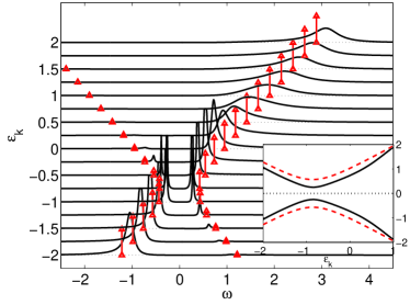
Figure 1: (Color online) The $\varepsilon_{{\bm{k}}}$-resolved spectral functions $\rho_{{\bm{k}}}(\omega)$ for $U=2$. The arrows show the delta-function peaks of the mean field result $\rho^{\rm BCS}_{{\bm{k}}}(\omega)$, where the height of the arrow indicates the weight of the peak. Inset: Mean field bands $E_{{\bm{k}}}^{0}$ (dashed) and real quasiparticle band $E_{{\bm{k}}}$ (full line).

We can see the two bands of quasiparticle excitations with the sharpest peaks in the region of minimal spectral gap. These spectra can be compared with the ones which were calculated by Garg et al.Garg et al. (2005) by iterated perturbation theory. There the quasiparticle excitation delta peaks are disconnected from the continuum, which is however an artifact of the approximation for the self-energy, whose imaginary part vanishes over too large a region in $\omega$. The mean field results (red arrows) describe the form of the quasiparticle bands qualitatively well. Also the weight of the peaks in the full spectrum $\rho_{{\bm{k}}}(\omega)$ is comparable with the height of the arrows of the mean field theory. Notice that the sharpest peaks of $\rho_{{\bm{k}}}(\omega)$ have the Lorentzian shape as in (12). For different $\varepsilon_{{\bm{k}}}$ and also at larger $U$ the peak form can be asymmetric and (12) not such a good fit.

The effect of the dynamic fluctuations on the excitation spectrum can be seen clearer in the inset of Fig. 1, where we compare the mean-field bands $E_{{\bm{k}}}^{0}$ with the real quasiparticle band $E_{{\bm{k}}}$. We can see a substantial reduction of the excitations energy for a certain bare energy $\varepsilon_{{\bm{k}}}$. For instance, the minimal spectral gap $\Delta_{\rm ex}=\min(E_{{\bm{k}}})$ is reduced by a factor of about $2.3$ in this case. For different values of the interaction in the whole crossover regime this reduction effect can be seen in Fig. 2, where we plot the value of the order parameter computed by mean field (MF) theory, $\Delta_{\rm sc,MF}$, and DMFT, $\Delta_{\rm sc,DMFT}$, and the spectral excitation gap $\Delta_{\rm ex}$. Note that only at weak coupling the minimal spectral gap is strictly given by $\Delta_{\rm ex}$, since at intermediate to stronger coupling there are broader peaks and one finds finite weight for $|\omega|<\Delta_{\rm ex}$ implying a smaller excitation gap.Bauer et al. (2009)

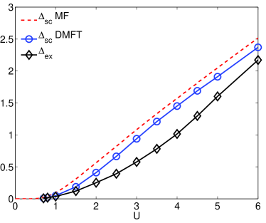
Figure 2: (Color online) Comparison of the order parameter $\Delta_{\rm sc}$ (mean field theory and DMFT) with spectral gap $\Delta_{\rm ex}$ for a range of interactions $U$.

The order parameter $\Delta_{\rm sc,DMFT}$ is reduced from its mean field value $\Delta_{\rm sc,MF}$ upon including fluctuations for all coupling strengths.Martin-Rodero and Flores (1992) Furthermore, we can see that the gap in the single particle spectrum $\Delta_{\rm ex}$, as deduced from the one particle Green’s function, is in turn smaller than $\Delta_{\rm sc,DMFT}$ for intermediate to strong coupling. At weak coupling these quantities tend to the same value suggesting an excitation spectrum of a renormalized mean field form.

In the weak coupling mean field theory the elementary excitations are gapped fermions. However, for strong coupling we deal with a bosonic system, and due to the large gap of order $U$ fermionic excitations are suppressed. We now analyze at which point in the intermediate coupling regime one tends to lose the sharp quasiparticle excitations. In order to study this question we look at the width of the excitations defined at the smallest spectral excitations $W=W(E_{{\bm{k}}}=\Delta_{\rm ex})$. If this is small we have a strongly peaked well-defined quasiparticle excitation as observed in Fig. 1, whereas for larger width the excitation decays more rapidly. For different local interaction strengths this is illustrated in Fig. 3.

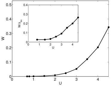
Figure 3: The quasiparticle width $W$ at the excitation gap energy for a range of interactions $U$. Inset: The ratio $W/\Delta_{\rm ex}$.

We find that whilst $W$ is very small for weak coupling it increases rapidly in the intermediate coupling regime, $U=2-4$. The ratio $W/\Delta_{\rm ex}$, which is plotted in the inset of Fig. 3, also increases from a small value at weak coupling to larger values at intermediate coupling. This shows that sharp (long-lived) quasiparticles excitations are suppressed then.

We now turn to spin and charge response functions. Within our framework we can calculate the local dynamic spin susceptibility $\chi_{s}(\omega)=(1/N)\sum_{{\bm{q}}}\chi_{s}(\omega,{\bm{q}})$ and charge susceptibility $\chi_{c}(\omega)$. The temperature dependence of $\chi_{s}$ in the static limit has been discussed by Keller et al.Keller et al. (2001) and the existence of a spin gap was demonstrated. In the following Fig. 4 we show the imaginary part of $\chi_{s}(\omega)$ (top) and $\chi_{c}(\omega)$ (bottom) for a number of values of $U$.

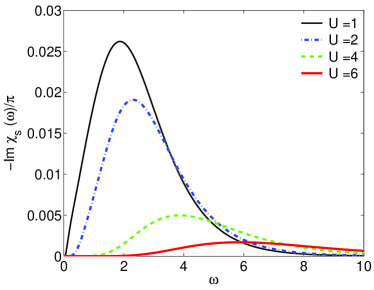
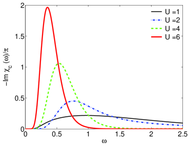
Figure 4: (Color online) The imaginary part of the local dynamic spin susceptibility $\chi_{s}(\omega)$ (top) and of the charge susceptibility $\chi_{c}(\omega)$ (bottom) for different $U$.

The spin response is suppressed when the local attraction $U$ is increased. The spin gapext $\Delta_{\rm sp}$ grows with $U$ as can be seen in the inset of Fig. 5, and it is directly related to the gap in the one particle excitation spectrum. This is expected since spin excitations are accompanied by breaking of a fermionic pair with opposite spin. For large $U$ the binding energy is proportional to $U$. The charge susceptibility shows a different behavior. The broad peak for weak coupling becomes sharper in the strong coupling limit and moves to lower energy. A similar trend is seen in the results for the charge susceptibility for ${\bm{q}}=0$ in the two dimensional model Kyung et al. (2006). A peak related to the massless Goldstone mode $\omega^{2}\sim{\bm{q}}^{2}$ is not present in our DMFT calculation for the local charge susceptibility. The visible charge gapext $\Delta_{\rm c}$, which is always smaller than the spin gap, first increases with $U$ but at strong coupling decreases again (see Fig. 5). The maximum occurs at a value, which is a bit larger than $U_{c}=2$ for the two-body bound state problem.

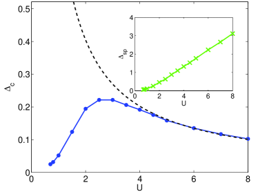
Figure 5: (Color online) The charge gap $\Delta_{\rm c}$ for a range of interactions $U$. The dashed line behaves $\sim 4t^{2}/U$. Inset: The spin gap as a function of $U$.

One way of understanding this behavior is to consider the mapping of the attractive Hubbard model to the half filled repulsive model in a magnetic field. At strong coupling this can be mapped to a Heisenberg model with spin coupling $J=4t^{2}/U$. Charge excitations in the attractive model correspond to spin excitations in the repulsive model, and the characteristic scale for the latter is $J$. The dashed line in Fig. 5 proportional to $4t^{2}/U$ with an adjusted prefactor reflects this dependence.

Perspective -

Let us comment on the range of applications of the extended DMFT-NRG method. Within this approach low temperature static and dynamic response functions can be calculated. In the experimental situation for the BCS-BEC crossover, the trapped fermionic gases constitute an inhomogeneous system. With a larger numerical effort these situations can be studied with real space DMFT extensions as done for the Mott transition Helmes et al. (2008). In the experiments it is difficult to cool the fermions down to very low temperatures compared to the Fermi energy. At finite temperature, but still in the symmetry-broken phase, the excitation gap is expected to be smaller compared to our $T=0$ case and the width of the quasiparticle excitation larger Singer et al. (1996). A calculation at finite temperature would be desirable to see how well the general features described here are still visible in the whole crossover regime.

Moreover, with the given method other models accessible by DMFT can be investigated. This includes, for instance, systems with a local electron phonon coupling, which are relevant to understand the fulleride superconductors. Also periodic Anderson type models and occurring superconducting phases are accessible.

Apart from these approximation to lattice models with a local self-energy, our method could also be used to study open problems for magnetic impurities in superconductors Balatsky et al. (2006). According to Anderson’s theorem and the work of Abrikosov and Gor’kov Abrikosov et al. (1963); Tinkham (1996) a finite concentration of non-magnetic impurities does not alter an s-wave superconducting state, but magnetic impurities suppress the order substantially. So far there are, however, few reliable quantitative microscopic studies of the local effect of a single impurity (magnetic or non-magnetic) on a superconductor. Since this is a non-perturbative problem our self-consistent NRG calculation could be an excellent method to tackle this problem. An attempt to investigate this based on the NRG method without self-consistency was made by Sakai et al. Sakai et al. (1993).

Conclusions -

We have applied an extended DMFT-NRG method to calculate self-consistent solutions with superconducting symmetry breaking in the attractive Hubbard model. This method can access static and dynamic quantities for any coupling strength and doping. We have focused on the zero temperature one particle spectrum and the local dynamic spin and charge susceptibilities for quarter filling. It was shown that the excitation energies are reduced substantially from their mean field results due to fluctuations. At weak coupling there are well-defined fermionic quasiparticle excitations, but as displayed in Fig. 3 the width of these excitation increases at intermediate coupling, such that sharp quasiparticle excitations are suppressed. In addition, the different behavior of the excitation gaps in the dynamic charge and spin susceptibilities has been analyzed quantitatively. We also pointed out that this work is not only relevant for the attractive Hubbard model, but the approach can be used to study superconductivity in other models, as well as for a microscopic description of the effect of impurities on superconductors.

Acknowledgment

We wish to thank N. Dupuis, P. Jakubczyk, W. Metzner, P. Strack and A. Toschi for helpful discussions, W. Koller and D. Meyer for their earlier contributions to the development of the NRG programs, and P. Strack for critically reading the manuscript.

References

- Bardeen et al. (1957) J. Bardeen, L. Cooper, and J. Schrieffer, Phys. Rev. 108, 1175 (1957).
- Greiner et al. (2003) M. Greiner, C. Regal, and D. Jin, Nature 426, 537 (2003).
- Zwierlein et al. (2004) M. Zwierlein, C. A. Stan, C. H. Schunck, S. M. F. Raupach, A. J. Kerman, and W. Ketterle, Phys. Rev. Lett. 92, 120403 (2004).
- Zwierlein et al. (2005) M. Zwierlein, J. Abo-Shaeer, A. Shirotzek, C. H. Schunck, and W. Ketterle, Nature 435, 1047 (2005).
- Bloch et al. (2008) I. Bloch, J. Dalibard, and W. Zwerger, Rev. Mod. Phys. 80, 885 (2008).
- Eagles (1969) D. M. Eagles, Phys. Rev. 186, 456 (1969).
- Leggett (1980) A. J. Leggett, in Modern Trends in the Theory of Condensed Matter, edited by A. Pekalski and R. Przystawa (Springer, Berlin, 1980).
- Nozières and Schmitt-Rink (1985) P. Nozières and S. Schmitt-Rink, J. Low Temp. Phys. 59, 195 (1985).
- Randeria (1995) M. Randeria, in Bose-Einstein Condensation, edited by A. Griffin, D. Snoke, and S. Strinagari (Cambridge University Press, Cambridge, 1995).
- Micnas et al. (1990) R. Micnas, J. Ranninger, and S.Robaszkiewicz, Rev. Mod. Phys. 62, 113 (1990).
- Toschi et al. (2005a) A. Toschi, M. Capone, and C. Castellani, Phys. Rev. B 72, 235118 (2005a).
- Chen et al. (2006) Q. Chen, K. Levin, and J. Stajic, J. Low Temp. Phys. 32, 406 (2006).
- Chin et al. (2004) C. Chin, M. Bartenstein, A. Altmeyer, S. Riedl, S. Jochim, J. Hecker Denschlag, and R. Grimm, Science 305, 1128 (2004).
- Greiner et al. (2005) M. Greiner, C. A. Regal, and D. S. Jin, Phys. Rev. Lett. 94, 070403 (2005).
- Keller et al. (2001) M. Keller, W. Metzner, and U. Schollwöck, Phys. Rev. Lett. 86, 4612 (2001).
- Capone et al. (2002) M. Capone, C. Castellani, and M. Grilli, Phys. Rev. Lett. 88, 126403 (2002).
- Garg et al. (2005) A. Garg, H. R. Krishnamurthy, and M. Randeria, Phys. Rev. B 72, 024517 (2005).
- Toschi et al. (2005b) A. Toschi, P. Barone, M. Capone, and C. Castellani, New J. Phys. 7, 7 (2005b).
- Singer et al. (1996) J. M. Singer, M. H. Pedersen, T. Schneider, H. Beck, and H.-G. Matuttis, Phys. Rev. B 54, 1286 (1996).
- Kyung et al. (2006) B. Kyung, A. Georges, and A.-M. S. Tremblay, Phys. Rev. B 74, 024501 (2006).
- Wilson (1975) K. Wilson, Rev. Mod. Phys. 47, 773 (1975).
- Hewson (1993) A. C. Hewson, The Kondo Problem to Heavy Fermions (Cambridge University Press, Cambridge, 1993).
- Sakai et al. (1989) O. Sakai, Y. Shimizu, and T. Kasuya, J. Phys. Soc. Japan 58, 3666 (1989).
- Costi et al. (1994) T. A. Costi, A. C. Hewson, and V. Zlatić, J. Phys.: Cond. Mat. 6, 2519 (1994).
- Georges et al. (1996) A. Georges, G. Kotliar, W. Krauth, and M. Rozenberg, Rev. Mod. Phys. 68, 13 (1996).
- Bulla et al. (1997) R. Bulla, T. Pruschke, and A. C. Hewson, J. Phys.: Cond. Mat. 9, 10463 (1997).
- Hofstetter (2000) W. Hofstetter, Phys. Rev. Lett. 85, 1508 (2000).
- Anders and Schiller (2005) F. B. Anders and A. Schiller, Phys. Rev. Lett. 95, 196801 (2005).
- Peters et al. (2006) R. Peters, T. Pruschke, and F. B. Anders, Phys. Rev. B 74, 245114 (2006).
- Weichselbaum and von Delft (2007) A. Weichselbaum and J. von Delft, Phys. Rev. Lett. 99, 076402 (2007).
- Bulla et al. (2008) R. Bulla, T. Costi, and T. Pruschke, Rev. Mod. Phys. 80, 395 (2008).
- Bulla (1999) R. Bulla, Phys. Rev. Lett. 83, 136 (1999).
- Zitzler et al. (2002) R. Zitzler, T. Pruschke, and R. Bulla, Eur. Phys. J. B 27, 473 (2002).
- Bauer and Hewson (2007) J. Bauer and A. C. Hewson, Eur. Phys. J. B 57, 235 (2007).
- Satori et al. (1992) K. Satori, H. Shiba, O. Sakai, and Y. Shimizu, J. Phys. Soc. Japan 61, 3239 (1992).
- Sakai et al. (1993) O. Sakai, Y. Shimizu, H. Shiba, and K. Satori, J. Phys. Soc. Japan 62, 3181 (1993).
- Bauer et al. (2007) J. Bauer, A. Oguri, and A. Hewson, J. Phys.: Cond. Mat. 19, 486211 (2007).
- Hecht et al. (2008) T. Hecht, A. Weichselbaum, J. von Delft, and R. Bulla, J. Phys.: Cond. Mat. 20, 275213 (2008).
- Yoshioka and Ohashi (2000) T. Yoshioka and Y. Ohashi, J. Phys. Soc. Japan 69, 1812 (2000).
- Choi et al. (2004) M.-S. Choi, M. Lee, K. Kang, and W. Belzig, Phys. Rev. B 70, 020502 (2004).
- Oguri et al. (2004) A. Oguri, Y. Tanaka, and A. C. Hewson, J. Phys. Soc. Japan 73, 2496 (2004).
- Bauer et al. (2009) J. Bauer, A. C. Hewson, and N. Dupuis (2009), cond-mat/0901.1760.
- (43) The following expansion is justified, when the imaginary parts of the self-energies are small and do not vary much near , which is satisfied in the weak coupling limit. However, as seen in Fig. 3 and Ref. BHD, such an analysis breaks down in the intermediate coupling regime. It would therefore be misleading to use the results for strong coupling.
- Martin-Rodero and Flores (1992) A. Martin-Rodero and F. Flores, Phys. Rev. B 45, 13008 (1992).
- (45) The gap in the dynamic response functions was extracted by taking the value of where the imaginary part of has increased from zero to of its maximal value.
- Helmes et al. (2008) R. W. Helmes, T. A. Costi, and A. Rosch, Phys. Rev. Lett. 100, 056403 (2008).
- Balatsky et al. (2006) A. V. Balatsky, I. Vekhter, and J.-X. Zhu, Rev. Mod. Phys. 78, 373 (2006).
- Abrikosov et al. (1963) A. A. Abrikosov, L. P. Gorkov, and I. E. Dzyaloshinski, Methods of quantum field theory in statistical physics (Dover, New York, 1963).
- Tinkham (1996) M. Tinkham, Introduction to Superconductivity (2nd edition) (Mc Grawth-Hill Inc., 1996).
- (50) J. Bauer, A.C. Hewson, and N. Dupuis, preprint in preparation (2008).