Physics results from dynamical overlap fermion simulations

Abstract:

I summarize the physics results obtained from large-scale dynamical overlap fermion simulations by the JLQCD and TWQCD collaborations. The numerical simulations are performed at a fixed global topological sector; the physics results in the $\theta$-vacuum is reconstructed by correcting the finite volume effect, for which the measurement of the topological susceptibility is crucial. Physics applications we studied so far include a calculation of chiral condensate, pion mass, decay constant, form factors, as well as (vector and axial-vector) vacuum polarization functions and nucleon sigma term.

1 Introduction

Many important aspects of the low energy dynamics of QCD are related to the chiral symmetry and its spontaneous breaking in the QCD vacuum. Lattice QCD is a promising tool to actually simulate the low energy regime of QCD and to reproduce the spontaneous symmetry breaking and related phenomena, provided that the chiral symmetry is preserved on the lattice. This was the prime motivation for the JLQCD and TWQCD collaborations to embark on the QCD simulations with exact chiral symmetry, i.e. dynamical overlap fermion simulations, despite the enormous computational costs they require.

Theoretically, with the dynamical overlap fermions, one may investigate the relation between chiral symmetry breaking and low-lying modes of the Dirac operator, as suggested by the Bank-Casher relation and the chiral random matrix theory. Also, the quantities related to the topology of the SU(3) gauge field, such as the topological susceptibility, may be studied using fermionic proves using the singlet axial-Ward-Takahashi identity.

Phenomenologically, the chiral symmetry plays an important role in the chiral extrapolation of lattice data for many physical quantities. Since the use of the continuum chiral perturbation theory is justified, the chiral extrapolation is largely simplified when the chiral symmetry is exactly preserved on the lattice. In this talk, I will discuss a few examples that demonstrate the chiral extrapolation performed using the next-to-next-to-leading order chiral perturbation theory formulae. We have other new applications for which the exact chiral symmetry plays a crucial role. They include a calculation of the $VV-AA$ vacuum polarization functions and an extraction of the strange quark content from the (partially quenched) nucleon masses.

This project was started in 2006 when the present supercomputer system, that comprises Hitachi SR11000 and IBM Blue Gene/L, was installed at KEK. A report of the project at an earlier stage was presented by Hideo Matsufuru at Lattice 2007 [1], which mainly described the simulation itself. The present talk discusses about the physics applications from the project in some detail. For individual contributions, see their own write-ups [2, 3, 4, 5, 6, 7, 8].

2 Simulation strategy and status

The overlap-Dirac operator $D(0)\equiv\rho/a[1+X/\sqrt{X^{\dagger}X}]$ (with the Wilson kernel $X\equiv aD_{W}-\rho$) [9, 10] provides a theoretically ideal fermion formulation on the lattice, as it has an exact chiral symmetry at finite lattice spacings [11] while satisfying the index theorem. Implementation of the overlap operator is however non-trivial, since the definition contains a discontinuity at the zero of the denominator $X^{\dagger}X$ (or the zero of the hermitian Wilson-Dirac operator $H_{W}\equiv\gamma_{5}X$). One usually approximates the sign function $\mathrm{sgn}(H_{W})$ using polynomial or rational functions, but the near-zero eigenmodes must be specially treated. At finite lattice spacings, it is known that there are finite density of near-zero modes of $H_{W}$ [12], that means that the computational cost to identify the near-zero modes grows as quickly as $O(V^{2})$ and prevents one from performing large scale simulations using the overlap fermion.

The near-zero modes are associated with a dislocation of the background gauge field and thus are unphysical (an explicit example is found in [13]). We suppress them by introducing extra heavy Wilson fermions (and associated ghosts) [14, 15]. They produce a factor $\det[H_{W}^{2}/(H_{W}^{2}+\mu^{2})]$ to the Boltzmann factor ($\mu$ is a mass of the associated ghosts) and naturally suppress the near-zero modes. The numerical cost for the overlap fermion simulation is then dramatically reduced especially when the lattice volume is large.

Since the topology change (or the change of the number of zero-modes of the overlap-Dirac operator) may occur only when a small eigenvalue of $H_{W}$ changes its sign, the suppression factor strictly prohibits the tunneling among different topological sectors, as far as the Monte Carlo algorithm is based on a continuous change of the gauge field configuration. This is in fact a property of the continuum QCD, i.e. topology change cannot occur through continuous deformation of the gauge field.

Dynamical overlap fermions have been attempted by several authors [16, 17, 18], in which the treatment of the topology tunneling is one of the main issues. Among them, our simulations have reached the level to produce broad physics results for the first time. On a lattice of size $\sim(\mbox{2~{}fm})^{3}$ we simulate dynamical fermions with several quark masses between $m_{s}/6$ and $m_{s}$ with $m_{s}$ the physical strange quark mass. In addition to the runs for two-flavor QCD, which is already published [19], we have completed a series of runs for 2+1-flavor QCD. The main reason that made this possible is the topology-fixing, as well as the computational power provided by the BlueGene/L.

The two-flavor runs were done at $\beta=2.30$ using the Iwasaki gauge action on a $16^{3}\times 32$ lattice. The lattice spacing determined through the Sommer scale $r_{0}$ = 0.49 fm is 0.118(2) fm. For each of six sea quark masses covering the region $m_{s}/6\sim m_{s}$, we accumulated 10,000 HMC trajectories in the trivial topological sector $Q=0$. (For a check of the fixed topology effect, we also produced configurations of $Q=-2$ and $-4$ at one sea quark mass. For details, see below.)

The 2+1-flavor runs were carried out at the same $\beta$ value on a $16^{3}\times 48$ lattice. This corresponds to the lattice spacing $a$ = 0.108(2) fm. We took two strange quark masses. For each of them, five up and down quark masses are taken covering the similar quark mass region. In total, ten runs of each length 2,500 HMC trajectories have been accumulated at $Q=0$.

3 Topology issues

If the topological charge is frozen in the QCD simulation, is there any problem? The answer to this question is obviously “yes”. The QCD vacuum is required to be the $\theta$-vacuum, a superposition of different topological sectors, in order to satisfy the cluster decomposition property. Therefore, we cannot sample the correct QCD vacuum unless the topological charge fluctuates sufficiently. This is a serious problem for everyone doing dynamical QCD simulation aiming at approaching the continuum limit, since the topological charge would not change near the continuum limit irrespective of which fermion formulation one employs.

We believe that the solution (one of the solutions, at least) to this problem is to reconstruct the $\theta$-vacuum physics from the fixed topology simulations [20]. This is based on the observation that the effect of fixed topological charge is a finite volume effect of $O(1/V)$, which can be derived from a simple Fourier transform between the $\theta$ vacuum and the fixed $Q$ “vacuum”. For instance, the partition function at a given topological charge $Q$ is obtained using a saddle point expansion as

$$Z_{Q}=\frac{1}{2\pi\chi_{t}V}\exp\left[-\frac{Q^{2}}{2\chi_{t}V}\right]\left[1-\frac{c_{4}}{8V\chi_{t}}+O\left(\frac{1}{(\chi_{t}V)^{2}},\frac{Q^{2}}{(\chi_{t}V)^{2}}\right)\right],$$ (1)

where $\chi_{t}$ is the topological susceptibility and $c_{4}$ characterizes a deviation from the Gaussian distribution at a finite volume. Therefore, if one can calculate $\chi_{t}$ and $c_{4}$ (and higher order terms if necessary), the $\theta$-vacuum can be reconstructed by simply adding the different topological sectors as $Z(\theta)=\sum_{Q}Z_{Q}e^{-i\theta Q}$. The method to calculate these key parameters is discussed shortly.

The relation between the $\theta$ and $Q$ vacuums can be extended to any physical quantities. For example, for a (CP-even) two-point function, one can express it in a given topological charge $Q$ in terms of its counterpart in the $\theta$(=0) vacuum $G(0)$ and its second and fourth derivatives $G^{(2)}(0)$ and $G^{(4)}(0)$ as [20, 21]

$$G_{Q}=G(0)+G^{(2)}(0)\frac{1}{2\chi_{t}V}\left[1-\frac{Q^{2}}{\chi_{t}V}-\frac{c_{4}}{2\chi_{t}^{2}V}\right]+G^{(4)}(0)\frac{1}{8\chi_{t}^{2}V^{2}}+\cdots$$ (2)

up to higher order corrections in $1/V$. Therefore, provided that the $\theta$-dependence of the quantity of interest is known, the $\theta$-vacuum physics can be reconstructed. The $\theta$-dependence can be obtained for the quantities that can be analysed using chiral perturbation theory; if it is not applicable one needs the data at several $Q$ to extract $G^{(2)}(0)$ for instance.

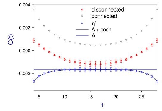
Figure 1: Pseudo-scalar density correlator (3) summed over spatial separation and plotted as a function of $t$. The data for $N_{f}=2$ QCD at $am=0.025$. Solid line shows a fit with a constant giving the topological susceptibility.

By applying the formula (2) for a topological charge density correlator, or equivalently a correlator of flavor-singlet pseudo-scalar densities $mP(x)$, one obtains a relation

$$\lim_{x\to\infty}\langle mP(x)mP(0)\rangle_{Q}=-\frac{1}{V}\left(\chi_{t}-\frac{Q^{2}}{V}+\cdots\right)+O(e^{-m_{\eta^{\prime}}x}),$$ (3)

where $\langle\cdots\rangle_{Q}$ stands for an expectation value in the given $Q$. The topological susceptibility $\chi_{t}$ can be extracted from the asymptotic value of the correlator in (3). One expects a negative constant when $Q=0$, which is intuitively understood as follows. When one finds a positive topological charge density at the origin, it is more likely that a negative value is observed at a far distant point $x$, if the net topology is fixed to $Q=0$. The value will be suppressed when the volume is increased.

An example obtained in two-flavor QCD is shown in Figure 1 [22]. We observe a clear plateau for all six different ensembles with different sea quark masses. At $am=0.050$, we obtain a consistent results from the configurations with different topological charges $Q=0$, $-2$, and $-4$.

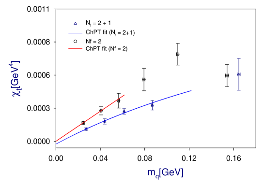
Figure 2: Topological susceptibility as a function of sea quark mass. The data for $N_{f}=2$ (circles) and $N_{f}=2+1$ (triangles) are shown. The solid curves represent a fit with the form of chiral effective theory.

Sea quark mass dependence of $\chi_{t}$ is expected to behave as $\chi_{t}=\Sigma/(1/m_{u}+1/m_{d}+1/m_{s})$ at the leading order of chiral perturbation theory [23]. In two-flavor QCD with degenerate sea quark mass $m$, it becomes $\chi_{t}=m\Sigma/2$. Figure 2 shows the results for 2- and 2+1-flavor QCD [2]. The data show a clear linear dependence on the sea quark mass. The fits to two- or 2+1-flavor formula yield the value of chiral condensate $\Sigma$. After a renormalization, we obtain $\Sigma(\mathrm{2~{}GeV})$ = [242(5)(10) MeV]³ ($N_{f}$=2) and $\Sigma(\mathrm{2~{}GeV})$ = [240(5)(2) MeV]³ ($N_{f}$=2+1).

4 Physics applications

4.1 Chiral condensate

For the lattice calculation of the chiral condensate, the exact chiral symmetry plays a crucial role. Without the exact symmetry the scalar density operator on the lattice $(\bar{\psi}\psi)^{lat}$ may mix with the identity operator under radiative corrections. This leads to a power (cubic) divergence in the matching onto the corresponding continuum operator $(\bar{\psi}\psi)^{cont}$, which prevents one from calculating this quantity on the lattice with any useful precision.

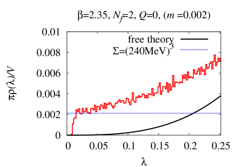
Figure 3: Spectral density $\rho(\lambda)$ as a function of $\lambda$, calculated from lattice data in the $\epsilon$-regime. Banks-Casher relation infers a constant at $\lambda=0$, which is not of course satisfied at a finite volume, but the remnant is clearly seen. The horizontal dashed line is an expectation for a nominal value of $\Sigma$.

Thanks to the exact chiral symmetry, we are able to precisely calculate this quantity from several different sources. They contain the use of the Banks-Casher relation (as demonstrated in Figure 3), the spectrum of low-lying eigenvalues (with a help of the chiral random matrix theory), the meson correlators in the $\epsilon$-regime, the topological susceptibility, and the Gell-Mann-Oaks-Renner (GMOR) relation.

In the $\epsilon$-regime, where pion Compton wavelength is longer than the spatial extent of the lattice, the dynamical degrees of freedom is dominated by the zero-momentum modes of pions. In this circumstance, the low-lying eigenmode spectrum can be obtained using the Chiral Random Matrix Theory (ChRMT). The chiral condensate can be extracted by matching the spectrum calculated on the lattice with the ChRMT prediction. We obtain $\Sigma^{\overline{\mathrm{MS}}}(\mathrm{2~{}GeV})$ = [251(7)(11) MeV]³ [24, 25]. The meson correlator calculated in the $\epsilon$-regime can also be used to determine the chiral condensate $\Sigma$ as well as the pion decay constant $F$. We obtain $\Sigma^{\overline{\mathrm{MS}}}(\mathrm{2~{}GeV})$ = [240(4)(7) MeV]³ and $F$ = 87(6)(8) MeV [26].

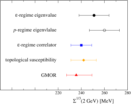
Figure 4: Chiral condensate calculated in two-flavor QCD with several different methods: $\epsilon$-regime eigenvalue spectrum [24, 25], $p$-regime eigenvalue spectrum [25], $\epsilon$-regime meson correlator [26], topological susceptibility [2], GMOR relation [27].

Figure 4 compares the chiral condensate extracted with various observables in two-flavor QCD. They are in good agreement. This strongly indicates that the low-energy dynamics of QCD is indeed determined by the pion degrees of freedom and therefore that the chiral symmetry is spontaneously broken, which is usually assumed when constructing the chiral effective theory.

4.2 $m_{\pi}$ and $f_{\pi}$

Near the massless limit of quarks the chiral effective theory is expected to provide a good description of the low-energy QCD. For larger pion masses, one must calculate loop corrections and also introduce irrelevant operators to subtract associated divergences. This leads to the chiral perturbation theory (ChPT), which is organized as an expansion in terms of small $m_{\pi}^{2}$ and $p^{2}$. The region of the convergence of this chiral expansion is not known a priori. Using lattice QCD, one can test the expansion and identify the region of convergence. With the exact chiral symmetry, the test is conceptually cleaner, since no additional term to describe the violation of chiral symmetry has to be introduced. (With other fermion formulations, this is not the case. The unknown correction terms are often simply ignored.)

For the pion mass $m_{\pi}$ and decay constant $f_{\pi}$ the expansion is given as

$$\frac{m_{\pi}^{2}}{m_{q}} = 2B\left[1+\frac{1}{2}x\ln x+c_{3}x+O(x^{2})\right],$$ (4)

$$f_{\pi} = f\left[1-x\ln x+c_{4}x+O(x^{2})\right],$$ (5)

where $m_{\pi}$ and $f_{\pi}$ denote the quantities after the corrections while $m$ and $f$ are them at the leading order. The expansions (4) and (5) may be written in terms of either $x\equiv 2m^{2}/(4\pi f)^{2}$, $\hat{x}\equiv 2m_{\pi}^{2}/(4\pi f)^{2}$, or $\xi\equiv 2m_{\pi}^{2}/(4\pi f_{\pi})^{2}$ (we use a notation of $f_{\pi}$ = 131 MeV). Theoretically, they all give an equivalent description at this order, while the convergence behavior may depend on the expansion parameter.

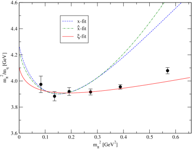
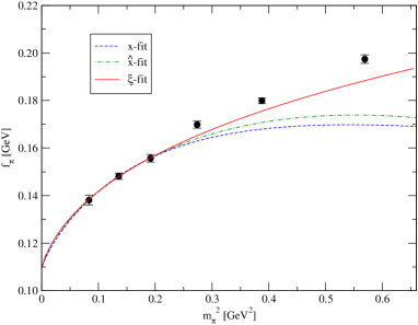
Figure 5: Comparison of chiral expansion in terms of $x$, $\hat{x}$ and $\xi$. The plots represent $m_{\pi}^{2}/m_{q}$ (left) and $f_{\pi}$ (right). Fits of the three lightest data points with the NLO ChPT formulae (4) and (5) are shown.

Figure 5 shows the comparison of different expansion parameters [27]. The fit curves are obtained by fitting the three lightest data points with the three different fit parameters. They all provide equally precise description of the data in the region of the fit. If we look at the heavier quark mass region, however, it is clear that only the $\xi$-expansion gives a reasonable function and others miss the data points largely. This clearly demonstrates that at least for these quantities the convergence of the chiral expansion is much improved by the use of the $\xi$-parameter than the conventional choice, i.e. the $x$-expansion.

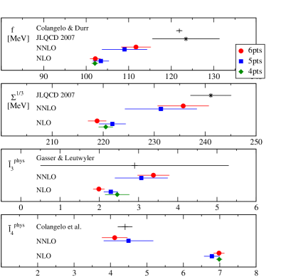
Figure 6: Low energy constants of two-flavor QCD as determined from the (N)NLO analysis of our lattice data. The results are obtained using 4, 5, or 6 lightest sea quark mass data. Phenomenological numbers are taken from Colangelo-Durr [29], Colangelo et al. [30]; the previous JLQCD results were obtained from the meson correlators in the $\epsilon$-regime [26].

Therefore, we consider only the $\xi$-expansion when we extend the analysis to the next-to-next-to-leading order (NNLO). I do not write down the NNLO terms here, but an important point is that the coefficient of the leading log terms of the form $(\xi\ln\xi)^{2}$ is determined solely from ChPT and thus is not a fit parameter. The terms of the form $\xi^{2}\ln\xi$ and $\xi^{2}$ have to be determined by the fit. It is indeed possible by a combined fit of $m_{\pi}^{2}/m_{q}$ and $f_{\pi}$; we obtain the low energy constants as shown in Figure 6.

It is clear from Figure 6 that the results depend on the order of the chiral expansion, i.e. NLO or NNLO, especially for the NLO low energy constants $\bar{\ell}_{3}$ and $\bar{\ell}_{4}$. This is because the NNLO term appears with a relatively large numerical coefficient, such as $\bar{\ell}_{3}\xi(1-9/2\xi\ln\xi)$, for instance. A large effect is then expected for the determination of $\bar{\ell}_{i}$ unless $\xi$ is much less than 0.1. The NNLO terms are mandatory in the analysis of lattice data.

We are currently extending the NNLO analysis to the partially quenched data in two-flavor QCD and to the 2+1-flavor QCD data [4].

4.3 Pion form factor

Pion vector and scalar form factors provide another simple testing ground for the chiral dynamics of pion. They are defined as

$$\langle\pi(p^{\prime})|V_{\mu}|\pi(p)\rangle = (p_{\mu}+p^{\prime}_{\mu})F_{V}(q^{2}),$$ (6)

$$\langle\pi(p^{\prime})|S|\pi(p)\rangle = F_{S}(q^{2}),\quad q_{\mu}\equiv p^{\prime}_{\mu}-p_{\mu},$$ (7)

for the vector current $V_{\mu}$ and the scalar density $S$. At small momentum transfer $q^{2}$, the form factors are characterized by the charge and scalar radii, $\langle r^{2}\rangle_{V}^{\pi}$, and $\langle r^{2}\rangle_{S}^{\pi}$, as

$$F_{V}(q^{2}) = 1+\frac{1}{6}\langle r^{2}\rangle_{V}^{\pi}q^{2}+O(q^{4}),$$ (8)

$$F_{S}(q^{2}) = F_{S}(0)\left[1+\frac{1}{6}\langle r^{2}\rangle_{S}^{\pi}q^{2}+O(q^{4})\right].$$ (9)

Note that the vector form factor $F_{V}(q^{2})$ is normalized at $q^{2}=0$ due to the current conservation.

We use the all-to-all quark propagator technique [31] to calculate the form factors [32, 7]. The main advantage of this technique is, of course, that one can calculate the disconnected diagram contribution to the scalar form factor. Furthermore, it substantially reduces the statistical error in the calculation through an average over the source point.

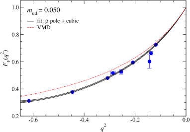
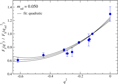
Figure 7: Pion vector (left) and scalar (right)form factors calculated at $am=0.050$.

We calculate the form factors at four lightest sea quark mass configurations available in two-flavor QCD. The data at a fixed quark mass are shown in Figure 7. For the vector form factor we attempt a fit ansatz motivated by the pole dominance $F_{V}(q^{2})=1/(1-q^{2}/m_{V}^{2})+c_{1}q^{2}+\cdots$ with $m_{V}$ the vector meson mass obtained at the same quark mass. This is justified by the analyticity of the form factor and also by a reasonable assumption that the higher pole contributions are well approximated by a Taylor series. The data are, in fact, nicely fitted with this function as shown in Figure 7 (left). The higher pole effects are small but visible. For the scalar form factor there is no obvious pole, and we use a simple polynomial of $q^{2}$ to fit the data (right panel).

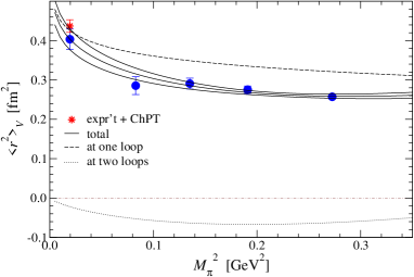
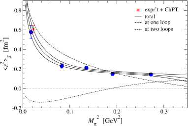
Figure 8: Vector (left) and scalar (right) radii of pion as a function of $M_{\pi}^{2}$. Solid curves show the fits with the NNLO ChPT formulae. Their breakdown into NLO (dashed) and NNLO (short dashed) contributions are also shown.

The charge and scalar radii thus extracted are plotted as a function of $m_{\pi}^{2}$ in Figure 8 together with the fits with the NNLO ChPT formulae. For these quantities, the ChPT predicts a logarithmic divergence in the chiral limit $\sim(1/f_{\pi}^{2})\ln m_{\pi}^{2}$ with a fixed numerical coefficient. The data do not show the expected divergent behavior, but the fit is possible and gives a value consistent with the phenomenological value at the point of physical pion mass. This suggests that the divergent behavior shows up in the even smaller quark mass region. We note that the fit is possible only when we include the NNLO terms, which contain additional logarithmic divergences in the chiral limit.

4.4 Vacuum polarization functions

The vacuum polarization functions defined through

$$\int d^{4}xe^{iqx}\langle 0|J_{\mu}(x)J_{\nu}^{\dagger}(0)|0\rangle=(g_{\mu}q^{2}-q_{\mu}q_{\nu})\Pi_{J}^{(1)}(Q^{2})-q_{\mu}q_{\nu}\Pi_{J}^{(0)}(Q^{2})$$ (10)

contain rich information of QCD dynamics in both perturbative and non-perturbative regimes. ($J_{\mu}$ is either a vector $V_{\mu}$ or an axial-vector $A_{\mu}$ current. We restrict ourselves in the flavor non-singlet currents, though the flavor indices are suppressed in the expressions.) Experimentally, the vacuum polarization function can be extracted from $e^{+}e^{-}$ annihilation or from $\tau$ decay processes.

The spontaneous chiral symmetry breaking can be probed with the vacuum polarization functions using the Weinberg sum rules [33], such as

$$f_{\pi}^{2} = -\lim_{Q^{2}\to 0}Q^{2}\left[\Pi_{V}^{(1+0)}(Q^{2})-\Pi_{A}^{(1+0)}(Q^{2})\right],$$ (11)

$$S = -\lim_{Q^{2}\to 0}\frac{\partial}{\partial Q^{2}}Q^{2}\left[\Pi_{V}^{(1+0)}(Q^{2})-\Pi_{A}^{(1+0)}(Q^{2})\right],$$ (12)

where $S$ stands for the Peskin-Takeuchi’s parameter used in the context of the precision electroweak measurement [34]. In chiral effective theory, it is related to a low energy constant $L_{10}$. These sum rules can be obtained in the limit of massless quarks. Because of their $VV-AA$ structure, they vanish when the chiral symmetry is not spontaneously broken.

Along these lines, another interesting quantity is the electromagnetic mass difference of pion, which is expressed in this limit as

$$\Delta m_{\pi}^{2}=-\frac{3\alpha_{EM}}{4\pi f_{\pi}^{2}}\int_{0}^{\infty}dQ^{2}Q^{2}\left[\Pi_{V}^{(1+0)}(Q^{2})-\Pi_{A}^{(1+0)}(Q^{2})\right],$$ (13)

which is known as the Das-Guralnik-Mathur-Low-Young sum rule [35].

For a lattice calculation of these quantities, exact chiral symmetry is essential, since we have to extract a tiny difference between the vector and axial-vector channels. In the calculation using the overlap fermions, we checked that even the lattice artifacts precisely cancel between $V$ and $A$ [36].

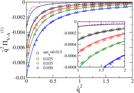
Figure 9: Difference of the vacuum polarization functions $\Pi_{V}^{(1)}(Q^{2})-\Pi_{A}^{(1)}(Q^{2})$ multiplied by $Q^{2}$. Data are shown for different quark masses; the chiral limit is also plotted by a solid (linear extrapolation) and a dashed (chiral logs) curve.

In Figure 9 we plot the results for the difference $\Pi_{V}^{(1)}(Q^{2})-\Pi_{A}^{(1)}(Q^{2})$. The chiral limit is taken by assuming a linear quark mass dependence (solid curve) or by using the one-loop ChPT formula (dashed curve). The use of ChPT is slightly questionable, because the lowest (non-zero) value of $Q^{2}$ on our lattice is already as large as (320 MeV)² and the second lowest $\sim$(650 MeV)² is clearly out of the range. The high $Q^{2}$ region, on the other hand, may be analyzed using the operator product expansion (OPE). OPE is also used to extend the region of $Q^{2}$ to infinity as required in (13). For the pion mass difference, we finally obtain $m_{\pi}^{2}$ = 992(12)(${}^{+\ \ 0}_{-135}$)(149) MeV² (see [36] for details), which may be compared with the experimental value 1,261 MeV².

Another use of the vacuum polarization function is an extraction of the strong coupling constant by matching the lattice data with the OPE expression in the perturbative regime. For this purpose we consider the Adler function $D_{J}(Q^{2})\equiv-Q^{2}d\Pi_{J}(Q^{2})/dQ^{2}$, which is free from ultraviolet divergence, and thus renormalization scheme independent. It means that one can use the expressions obtained in the continuum perturbation theory to describe the lattice data. (In the practical analysis, we directly use $\Pi_{J}(Q^{2})$ instead, to avoid numerical derivative in terms of $Q^{2}$. We then float a divergent constant as a fit parameter.)

In the lattice calculation, it is necessary to subtract lattice artifacts mainly due to non-conserved lattice currents. Non-perturbative subtraction is possible by utilizing several different momentum configurations giving the same $Q^{2}$ [37].

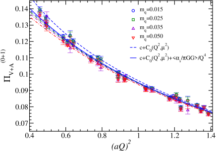
Figure 10: Vacuum polarization function $\Pi_{V+A}^{(1)}(Q^{2})$ as a function of $Q^{2}$. The lattice data at different quark masses are shown together with the fit curve with the OPE formula (solid curve).

Lattice results are shown in Figure 10. The data in high $Q^{2}$ regime are fitted with the perturbative expression supplemented by OPE

$$\Pi_{J}^{\mathrm{pert}}(Q^{2})=c+C_{0}(Q^{2},\mu^{2})+\frac{C_{m}^{J}(Q^{2})}{Q^{2}}+C_{\bar{q}q}^{J}(Q^{2})\frac{\langle m\bar{q}q\rangle}{Q^{4}}+C_{GG}(Q^{2})\frac{\langle(\alpha_{s}/\pi)GG\rangle}{Q^{4}}+\cdots,$$ (14)

where perturbative expansion of $C_{0}$, $C_{m}$, etc is known to $\alpha_{s}^{2}$ in the $\overline{\mathrm{MS}}$ scheme. $c$ is the divergent constant term.

In the analysis, we may use the value of the chiral condensate $\langle\bar{q}q\rangle$ obtained through other quantities as described above. We then obtain $\Lambda_{\overline{\mathrm{MS}}}^{(2)}$ = 234(9)(${}^{+16}_{-\ 0}$) MeV in two-flavor QCD [37]. This result is compatible with previous lattice calculations in two-flavor QCD, 250(16)(16) MeV [38] or 249(16)(25) MeV [39].

4.5 Nucleon structure

The last application of our dynamical overlap fermion simulations reported in this talk is a calculation of the nucleon sigma term

$$\sigma_{\pi N}=m_{ud}\langle N|\bar{u}u+\bar{d}d|N\rangle$$ (15)

and the strange quark content

$$y=\frac{2\langle N|\bar{s}s|N\rangle}{\langle N|\bar{u}u+\bar{d}d|N\rangle}.$$ (16)

For $\sigma_{\pi N}$ both connected and disconnected quark lines contribute, while only the disconnected diagram contributes to the strange quark content.

Instead of directly calculating the matrix elements in (15) and (16), we utilize the Feynman-Hellman theorem. Namely, we calculate the derivatives of nucleon mass in terms of valence or sea quark mass. They are related to the connected and disconnected contributions as

$$\frac{\partial M_{N}}{\partial m_{\mathrm{val}}} = \langle N|\bar{u}u+\bar{d}d|N\rangle_{\mathrm{conn}},$$ (17)

$$\frac{\partial M_{N}}{\partial m_{\mathrm{sea}}} = \langle N|\bar{u}u+\bar{d}d|N\rangle_{\mathrm{disc}}(\simeq 2\langle N|\bar{s}s|N\rangle),$$ (18)

where the subscripts “conn” and “disc” stand for the connected and disconnected contributions to the matrix element, respectively. The disconnected piece becomes identical to the strange matrix element $2\langle N|\bar{s}s|N\rangle$ when the sea quark mass is set equal to the strange quark mass. To obtain the derivatives we need partially quenched ($m_{\mathrm{val}}\neq m_{\mathrm{sea}}$) data set. For the fit of the quark mass dependence, we use the partially quenched chiral perturbation theory calculated at one-loop for the nucleon mass [40, 41].

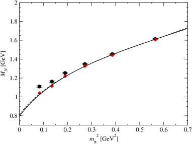
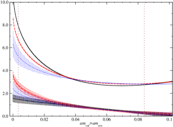
Figure 11: (Left) Nucleon mass in two-flavor QCD. The data after the finite volume correction are shown by red symbols. The curves represent the fit with baryon ChPT formulae. (Right) The connected (upper) and disconnected (lower) contributions to the sigma term as a function of the quark mass. Sea and valence quarks are taken to be equal. Physical up/down and strange quark masses are shown by vertical lines.

Figure 11 (left panel) shows the nucleon mass calculated on our two-flavor QCD configurations as a function of $m_{\pi}^{2}$ [42]. Finite volume effect is corrected using the expectation from ChPT [43]. The data are nicely fitted with the ChPT formula at $O(p^{3})$ or at $O(p^{4})$, through which we obtain $\sigma_{\pi N}$ = 52(2)(${}^{+20}_{-\ 2}$)(${}^{+5}_{-0}$) MeV (for further details, see [42]).

The derivatives can be obtained after fitting the partially quenched data set with the corresponding ChPT formulae. The results are shown in Figure 11 (right panel). The plot clearly shows that the disconnected contribution is smaller than the connected contribution. In particular, the disconnected piece is tiny for the mass corresponding to the strange quark. As a result the $y$ parameter we obtained is small: $y$ = 0.030(16)(${}^{+6}_{-8}$)(${}^{+1}_{-2}$).

Previous lattice calculations gave rather large values for $y$: 0.66(15) [44], 0.36(3) [45], 0.59(13) [46]. The problem in these calculations is that the critical mass depend significantly on the sea quark mass when one uses the Wilson-type fermion due to the lack of chiral symmetry. One can misidentify this unphysical effect with the physical sigma term. (We note that the problem persists even when one directly calculates the matrix element rather than using the Feynman-Hellman theorem. That is because the scalar density operator made up with valence quarks may mix with that with sea quarks. One has to subtract this operator mixing to obtain the correct results [5].)

After subtracting this effect, UKQCD obtained a value consistent with zero, $y=-0.28(33)$, albeit a large error due to the subtraction [47]. Our setup is free from this problem because of the use of the overlap fermion for both valence and sea quarks. The exact chiral symmetry plays a key role here, too.

5 Conclusions

In this talk I demonstrate that the dynamical overlap fermion may provide a clean approach to the problems related to the chiral symmetry and its spontaneous breaking. Despite the large numerical cost it requires, large scale simulation is feasible with the computational resources of $O$(10 TFlops). So far, we have completed runs on a 16${}^{3}\times$48 and started test runs on a larger volume, 24${}^{3}\times$48.

The key to this success is the new strategy of treating the global topological charge. i.e. we fix the topology during the simulation and reproduce the $\theta$-vacuum physics by correcting an induced finite volume effect. In doing so, the key observation is that the topological susceptibility can be correctly extracted from simulations at a fixed topology.

The problem of topology freezing will become common among all lattice simulations as one sufficiently approaches the continuum limit, simply because this is the property of the continuum QCD. Our work is a first attempt to overcome that situation.

The exact chiral symmetry plays a crucial role in the calculation of many important physical quantities. For instance, we have calculated the chiral condensate using several methods for the first time and confirmed the consistency among them, which provides the most fundamental test of the chiral effective theory. We are extending the test to various quantities, such as pion mass, decay constant, charge radius and so on. (A calculation of the kaon $B$ parameter is already published [48].) There are other interesting applications for which the exact chiral symmetry is required; so far we studied the $VV-AA$ vacuum polarization and the nucleon sigma term. We plan to further pursue in this direction.

The author is supported in part by Grant-in-aid for Scientific Research (No. 18340075).

References

- [1] H. Matsufuru [JLQCD and TWQCD Collaborations], PoS LAT2007 (2007) 018 [arXiv:0710.4225 [hep-lat]].
- [2] T. W. Chiu et al. [JLQCD and TWQCD Collaborations], PoS LAT2008 (2008) 072; arXiv:0810.0085 [hep-lat].
- [3] H. Matsufuru et al. [JLQCD and TWQCD Collaborations], PoS LAT2008 (2008) 077.
- [4] J. Noaki et al. [JLQCD and TWQCD collaborations], PoS LAT2008 (2008) 107; arXiv:0810.1360 [hep-lat].
- [5] H. Ohki et al. [JLQCD Collaboration], PoS LAT2008 (2008) 126; arXiv:0810.4223 [hep-lat].
- [6] E. Shintani et al. [JLQCD and TWQCD Collaborations], PoS LAT2008 (2008) 134.
- [7] T. Kaneko et al. [JLQCD and TWQCD Collaborations], PoS LAT2008 (2008) 158; arXiv:0810.2590 [hep-lat].
- [8] N. Yamada et al. [JLQCD and TWQCD Collaborations], PoS LAT2008 (2008) 284.
- [9] H. Neuberger, Phys. Lett. B 417, 141 (1998) [arXiv:hep-lat/9707022].
- [10] H. Neuberger, Phys. Lett. B 427, 353 (1998) [arXiv:hep-lat/9801031].
- [11] M. Luscher, Phys. Lett. B 428, 342 (1998) [arXiv:hep-lat/9802011].
- [12] R. G. Edwards, U. M. Heller and R. Narayanan, Nucl. Phys. B 535 (1998) 403 [arXiv:hep-lat/9802016].
- [13] F. Berruto, R. Narayanan and H. Neuberger, Phys. Lett. B 489 (2000) 243 [arXiv:hep-lat/0006030].
- [14] P. M. Vranas, Phys. Rev. D 74 (2006) 034512 [arXiv:hep-lat/0606014].
- [15] H. Fukaya, S. Hashimoto, K. I. Ishikawa, T. Kaneko, H. Matsufuru, T. Onogi and N. Yamada [JLQCD Collaboration], Phys. Rev. D 74 (2006) 094505 [arXiv:hep-lat/0607020].
- [16] Z. Fodor, S. D. Katz and K. K. Szabo, JHEP 0408 (2004) 003 [arXiv:hep-lat/0311010].
- [17] T. A. DeGrand and S. Schaefer, Phys. Rev. D 71 (2005) 034507 [arXiv:hep-lat/0412005].
- [18] N. Cundy, S. Krieg, G. Arnold, A. Frommer, T. Lippert and K. Schilling, arXiv:hep-lat/0502007.
- [19] S. Aoki et al. [JLQCD Collaboration], Phys. Rev. D 71 (2008) 014508 [arXiv:0803.3197 [hep-lat]].
- [20] S. Aoki, H. Fukaya, S. Hashimoto and T. Onogi, Phys. Rev. D 76 (2007) 054508 [arXiv:0707.0396 [hep-lat]].
- [21] R. Brower, S. Chandrasekharan, J. W. Negele and U. J. Wiese, Phys. Lett. B 560 (2003) 64 [arXiv:hep-lat/0302005].
- [22] S. Aoki et al. [JLQCD and TWQCD Collaborations], Phys. Lett. B 665 (2008) 294 [arXiv:0710.1130 [hep-lat]].
- [23] H. Leutwyler and A. V. Smilga, Phys. Rev. D 46 (1992) 5607.
- [24] H. Fukaya et al. [JLQCD Collaboration], Phys. Rev. Lett. 98 (2007) 172001 [arXiv:hep-lat/0702003].
- [25] H. Fukaya et al. [JLQCD and TWQCD Collaborations], Phys. Rev. D 76 (2007) 054503 [arXiv:0705.3322 [hep-lat]].
- [26] H. Fukaya et al. [JLQCD collaboration], Phys. Rev. D 77 (2008) 074503 [arXiv:0711.4965 [hep-lat]].
- [27] J. Noaki et al. [JLQCD and TWQCD Collaborations], arXiv:0806.0894 [hep-lat].
- [28] J. Gasser and H. Leutwyler, Annals Phys. 158, 142 (1984).
- [29] G. Colangelo and S. Durr, Eur. Phys. J. C 33 (2004) 543 [arXiv:hep-lat/0311023].
- [30] G. Colangelo, J. Gasser and H. Leutwyler, Nucl. Phys. B 603 (2001) 125 [arXiv:hep-ph/0103088].
- [31] J. Foley, K. Jimmy Juge, A. O’Cais, M. Peardon, S. M. Ryan and J. I. Skullerud, Comput. Phys. Commun. 172 (2005) 145 [arXiv:hep-lat/0505023].
- [32] T. Kaneko, H. Fukaya, S. Hashimoto, H. Matsufuru, J. Noaki, T. Onogi and N. Yamada [JLQCD collaboration], PoS LAT2007 (2007) 148 [arXiv:0710.2390 [hep-lat]].
- [33] S. Weinberg, Phys. Rev. Lett. 18 (1967) 507.
- [34] M. E. Peskin and T. Takeuchi, Phys. Rev. Lett. 65 (1990) 964.
- [35] T. Das, G. S. Guralnik, V. S. Mathur, F. E. Low and J. E. Young, Phys. Rev. Lett. 18 (1967) 759.
- [36] E. Shintani et al. [JLQCD Collaboration], arXiv:0806.4222 [hep-lat].
- [37] E. Shintani et al. [JLQCD and TWQCD Collaborations], arXiv:0807.0556 [hep-lat].
- [38] M. Della Morte, R. Frezzotti, J. Heitger, J. Rolf, R. Sommer and U. Wolff [ALPHA Collaboration], Nucl. Phys. B 713 (2005) 378 [arXiv:hep-lat/0411025].
- [39] M. Gockeler, R. Horsley, A. C. Irving, D. Pleiter, P. E. L. Rakow, G. Schierholz and H. Stuben, Phys. Rev. D 73 (2006) 014513 [arXiv:hep-ph/0502212].
- [40] J. W. Chen and M. J. Savage, Phys. Rev. D 65 (2002) 094001 [arXiv:hep-lat/0111050].
- [41] S. R. Beane and M. J. Savage, Nucl. Phys. A 709 (2002) 319 [arXiv:hep-lat/0203003].
- [42] H. Ohki et al. [JLQCD Collaboration], arXiv:0806.4744 [hep-lat].
- [43] A. Ali Khan et al. [QCDSF-UKQCD Collaboration], Nucl. Phys. B 689 (2004) 175 [arXiv:hep-lat/0312030].
- [44] M. Fukugita, Y. Kuramashi, M. Okawa and A. Ukawa, Phys. Rev. D 51 (1995) 5319 [arXiv:hep-lat/9408002].
- [45] S. J. Dong, J. F. Lagae and K. F. Liu, Phys. Rev. D 54 (1996) 5496 [arXiv:hep-ph/9602259].
- [46] S. Gusken et al. [TXL Collaboration], Phys. Rev. D 59 (1999) 054504 [arXiv:hep-lat/9809066].
- [47] C. Michael, C. McNeile and D. Hepburn [UKQCD Collaboration], Nucl. Phys. Proc. Suppl. 106 (2002) 293 [arXiv:hep-lat/0109028].
- [48] S. Aoki et al. [JLQCD Collaboration], Phys. Rev. D 77 (2008) 094503 [arXiv:0801.4186 [hep-lat]].