Wavelet domain Bayesian denoising of string signal in the cosmic microwave background

Abstract

An algorithm is proposed for denoising the signal induced by cosmic strings in the cosmic microwave background (CMB). A Bayesian approach is taken, based on modeling the string signal in the wavelet domain with generalized Gaussian distributions. Good performance of the algorithm is demonstrated by simulated experiments at arcminute resolution under noise conditions including primary and secondary CMB anisotropies, as well as instrumental noise.

1 Introduction

Observations of the cosmic microwave background (CMB) and of the Large Scale Structure of the Universe (LSS) have led to the definition of a concordance cosmological model. Recently, analysis of the temperature data of the CMB over the whole celestial sphere from the Wilkinson Microwave Anisotropy Probe (WMAP) satellite experiment has played a dominant role in designing this precise picture of the Universe (Bennett et al., 2003; Spergel et al., 2003; Hinshaw et al., 2007; Spergel et al., 2007; Hinshaw et al., 2009; Komatsu et al., 2009). Experiments dedicated to the observation of small portions of the celestial sphere have also provided their contribution, including the Arcminute Cosmology Bolometer Array Receiver (ACBAR) experiment (Reichardt et al., 2009), the Boomerang experiment (Jones et al., 2006), and the Cosmic Background Imager (CBI) experiment (Readhead et al., 2004).

According to the concordance cosmological model, the cosmic structures and the CMB originate from Gaussian adiabatic perturbations seeded in the early phase of inflation of the Universe. However, cosmological scenarios motivated by theories for the unification of the fundamental interactions predict the existence of topological defects resulting from phase transitions at the end of inflation (Vilenkin & Shellard, 1994; Hindmarsh, 1995a; Hindmarsh & Kibble, 1995b; Turok & Spergel, 1990). These defects would have participated to the formation of the cosmic structures, also imprinting the CMB. In particular, cosmic strings are a line-like version of such defects which are also predicted in the framework of fundamental string theory (Davis & Kibble, 2005). As a consequence, the issue of their existence is a central question in cosmology today.

Cosmic strings are parametrized by a string tension $\mu$, i.e. a mass per unit length of string, which sets the overall amplitude of the contribution of a string network. Their main signature in the CMB is characterized by temperature steps along the string positions. This localized effect, known as the Kaiser-Stebbins (KS) effect (Kaiser & Stebbins, 1984; Gott, 1985), hence implies a non-Gaussian imprint of the string network in the CMB. The most numerous strings appear at an angular size around $1$ degree on the celestial sphere. CMB experiments with an angular resolution much below $1$ degree are thus required in order to resolve the width of cosmic strings.

Experimental constraints have been obtained on a possible string contribution in terms of upper bounds on the string tension $\mu$ (Perivolaropoulos, 1993; Bevis et al., 2004; Wyman et al., 2005, 2006; Bevis et al., 2007; Fraisse et al., 2007). In this context, even though observations largely fit with an origin of the cosmic structures in terms adiabatic perturbations, room is still available for the existence of cosmic strings.

The purpose of the present work is to develop an effective method for mapping the string network potentially imprinted at high angular resolution in CMB temperature data, in the perspective of forthcoming arcminute resolution experiments. The observed CMB signal can be modeled as a linear superposition of a statistically isotropic but non-Gaussian string signal proportional to an unknown string tension, with statistically isotropic Gaussian noise comprising the standard component of the CMB induced by adiabatic perturbations as well as instrumental noise.

We take a Bayesian approach to this denoising problem, based on statistical models for both the string signal and noise. Our denoising is done in the wavelet domain, using a steerable wavelet transform well adapted for representing the strongly oriented features present in the string signal. We show that the string signal coefficients are well described by generalized Gaussian distributions (GGD’s), which are fit at each wavelet scale using a training simulation borrowed from the set of realistic string simulations recently produced by Fraisse et al. (2008).

We develop a Bayesian least squares method for the denoising, where each coefficient of the wavelet decomposition is estimated as the expectation value of its posterior probability distribution given the observed value. This estimation is split into two parts. Assuming the string tension is known, we use the GGD model to compute an estimate of the string signal. However, the true string tension is unknown. We deal with this by using a preliminary power spectral model (PSM) to calculate a posterior probability for the string tension. We then construct our overall estimator by weighting the GGD based estimators using this posterior probability distribution for the string tension. Finally, the string network itself can be mapped by taking the magnitude of the gradient of the denoised signal (Fraisse et al., 2008).

The denoising algorithm that we present may be considered as a modular component of a larger data analysis. Firstly notice that the PSM might be replaced by any other model allowing computation of the posterior probability distribution of the string tension, notably those which rely on the best experimental bounds on the string tension. Secondly, as our method produces a temperature map of the same size as the input, it may also find use as a pre-processing step for other methods for cosmic string detection based on explicit edge detection (Jeong & Smoot, 2005; Lo & Wright, 2005; Amsel et al., 2007).

The performance of our denoising algorithm is evaluated under different conditions, with astrophysical noise components including various contributions to the standard component of the CMB (i.e. primary and secondary CMB anisotropies), as well as instrumental noise. Three quantitative measures of performance are considered, namely the signal-to-noise ratio, correlation coefficient, and kurtosis of the magnitude of gradient of the string signal. Our analyses rely on $100$ test simulations of a string signal buried in the noise. For each string tension and noise condition considered, the test simulations are produced by linear superposition of a unique test string simulation, also from (Fraisse et al., 2008), with independent noise realizations.

In each noise condition, we find that the lowest values for the string tension down to which our quantitative measures show effective denoising are very close to the lowest value where strings begin to be visible by eye. Moreover, we acknowledge that this value is slightly larger than a detectability threshold set on the basis of the PSM.

The remainder of this paper is organized as follows. In Section 2, we discuss the string signal and the noise at arcminute resolution, and we describe our numerical simulations. In Section 3, we describe the steerable wavelet formalism on the plane and study the sparsity of the string signal in terms of the wavelet decomposition. In Section 4, we define in detail our wavelet domain Bayesian denoising (WDBD) algorithm. In Section 5, we evaluate the performance of the algorithm. We finally conclude in Section 6.

2 String signal and noise

In this section, we describe the string signal, discuss current and expected future experimental constraints, and detail the various noise components at arcminute resolution. We also describe the numerical simulations used for our developments.

2.1 String signal

In an inflationary cosmological model, the phase transitions responsible for the formation of a cosmic string network occur after the end of inflation, so as to produce observable defects. From the epoch of last scattering until today, the cosmic string network continuously imprints the CMB. The so-called scaling solution for the string network implies that the most numerous strings are imprinted just after last scattering and have a typical angular size around $1$ degree, of the order of the horizon size at that time (Vachaspati & Vilenkin, 1984; Kibble, 1985; Albrecht & Turok, 1985; Bennet, 1986; Bennet & Bouchet, 1989; Albrecht & Turok, 1989; Bennet & Bouchet, 1990; Allen & Shellard, 1990). Longer strings are also imprinted in the later stages of the Universe evolution, but in smaller number, according to the number of corresponding horizon volumes required to fill the sky.

The main signature of a cosmic string in the CMB is described by the KS effect according to which a temperature step is induced in the CMB along the string position. The relative amplitude of this step reads as

$$\frac{\delta T}{T}=\left(8\pi\gamma\beta\right)\rho,$$ (1)

where $\beta=v/c$, $\gamma=(1-\beta^{2})^{-1/2}$ is the relativistic gamma factor, and $\rho$ is a dimensionless parameter uniquely associated with the string tension $\mu$ through

$$\rho=\frac{G\mu}{c^{2}},$$ (2)

where $G$ stands for the gravitational constant and $c$ for the speed of light. In the following we call $\rho$ the string tension.

Analytical models relying on the KS effect and the scaling property were defined to simulate the string signal imprinted in the CMB. However, in order to produce precise CMB maps accounting for the full non-linear evolution of the string network, one needs to resort to numerical simulations. On small angular scales, realistic simulations can be produced by stacking CMB maps induced in different redshift ranges between last scattering and today. The simulations we use in this work have been produced by this technique (Bouchet et al., 1988; Fraisse et al., 2008).

The string signal is understood as a realization of a statistically isotropic but non-Gaussian process on the celestial sphere with an overall amplitude rescaled by the string tension $\rho$, and characterized by a nearly scale-free angular power spectrum: $C_{l}^{s}(\rho)=\rho^{2}C_{l}^{s}$, where the positive integer index $l$ stands for the angular frequency index on the sphere. An analytical expression of this spectrum was provided for $l$ larger than a few hundreds by Fraisse et al. (2008), on the basis of their simulations. We consider CMB experiments with a small field of view corresponding to an angular opening $\tau\in[0,2\pi)$ on the celestial sphere. In this context, the small portion of the celestial sphere accessible is identified to a planar patch of size $\tau\times\tau$, and we may consider planar signals in terms of Cartesian coordinates $\textbf{\em x}=(x,y)$. The spatial frequencies may be denoted as $\textbf{\em k}=(k_{x},k_{y})$ with a radial component $k=(k_{x}^{2}+k_{y}^{2})^{1/2}$. In this Euclidean limit, the radial component identifies with the angular frequency on the celestial sphere, below some band limit set by the resolution of the experiment under consideration: $l=k<B$. Analogously, the planar power spectrum, depending only on the radial component $k$ for a statistically isotropic signal, identifies with the angular power spectrum of the original signal on the sphere. In particular, for $k$ larger than a few hundreds, the nearly scale-free planar power spectrum of the string signal $s(\textbf{\em x})$ reads as

$$P^{s}\left(k,\rho\right)=\rho^{2}P^{s}\left(k\right),$$ (3)

with $P^{s}(k)=C_{l}^{s}$ for $l=k$.

In this context, the observed CMB signal can be understood as a linear superposition of the string signal and statistically isotropic noise of astrophysical and instrumental origin. As will be discussed in detail below, this noise is modeled as Gaussian with some angular power spectrum $C_{l}^{n}$. In the Euclidean limit, the corresponding planar power spectrum for the noise $n(\textbf{\em x})$ may be written as $P^{n}(k)=C_{l}^{n}$ for $l=k$. The observed noisy signal $f(\textbf{\em x})$ is given by:

$$f\left(\textbf{\em x}\right)=s\left(\textbf{\em x}\right)+n\left(\textbf{\em x}\right).$$ (4)

Let us notice that we consider zero mean signals, identifying perturbations around statistical means.

2.2 Experimental constraints

Current CMB experiments achieve an angular resolution on the celestial sphere of the order of $10$ arcminutes, corresponding to a limit angular frequency not far above $B\simeq 10^{3}$. At such resolutions, the standard component of the CMB primarily contains the Gaussian perturbations induced by adiabatic perturbations at last scattering, i.e. when the Universe became essentially transparent to radiation. These Gaussian anisotropies are referred to as the primary CMB anisotropies. In this context, any possible string signal is confined to amplitudes largely dominated by these primary anisotropies. The constraints mainly come from a best fit analysis of the angular power spectrum of the overall CMB signal in the WMAP temperature data (Perivolaropoulos, 1993; Bevis et al., 2004; Wyman et al., 2005, 2006; Bevis et al., 2007; Fraisse et al., 2007). The tightest of these constraints (Fraisse et al., 2007) gives the following upper bound at $68$ per cent confidence level:

$$\rho\leq\rho_{\mbox{{\scriptsize exp}}}=2.1\times 10^{-7}.$$ (5)

Algorithms have also been designed for the explicit identification of cosmic strings through the observation of the KS effect on CMB temperature data. The results of the analysis of the full-sky WMAP data typically provide constraints on the string tension two orders of magnitude wider than the best fit analysis of the CMB angular power spectrum, i.e. roughly $\rho<10^{-5}$ (Jeong & Smoot, 2005; Lo & Wright, 2005). The limited angular resolution of the WMAP data relative to a typical string width is actually more harmful for the explicit local detection of cosmic strings than for the estimation of a global parameter such as the string tension through the analysis of an angular power spectrum. Corresponding bounds have also been studied in the perspective of experiments providing higher resolution observation of the CMB on small portions of the sky (Amsel et al., 2007).

2.3 Noise at arcminute resolution

\psfrag{1e+04}{$10^{4}$}\psfrag{1e+03}{$10^{3}$}\psfrag{1e+02}{$10^{2}$}\psfrag{1e+00}{$1$}\psfrag{1e-02}{$10^{-2}$}\includegraphics[width=227.62204pt]{figures/figure1_psgraph}

Figure 1: Angular power spectra of string signal and noise (borrowed from Fraisse et al. (2008)) as a function of angular frequency in the range $l\in[10^{2},2\times 10^{4}]$ in $\log_{10}-\log_{10}$ axes scaling. The spectrum of the string signal is represented for a string tension $\rho=2\times 10^{-7}$ in terms of its analytical expression valid at high angular frequencies (red straight line). The noise spectra (ordered by decreasing amplitude at low angular frequencies) are: the primary CMB anisotropies (black solid line) and the gravitational lensing correction (black dashed line), the thermal SZ effect in the Rayleigh-Jeans limit (blue solid line), the non-linear kinetic SZ effect (green solid line), and the Ostriker-Vishniac effect (magenta solid line).

Forthcoming experiments will provide access to higher angular resolution. The Planck Surveyor satellite experiment will provide full-sky CMB data at a resolution of $5$ arcminutes, i.e. with $B\simeq 2\times 10^{3}$ (Bouchet, 2004) . The Atacama Cosmology Telescope (ACT) (Kosowsky, 2006), or the South Pole Telescope (SPT) (Ruhl et al., 2004) will map the CMB on small portions of the celestial sphere at a resolution around $1$ arcminute, i.e. with $B\simeq 10^{4}$. A slightly higher resolution might be reached by the radio interferometer Arcminute Microkelvin Imager (AMI) (Jones et al., 2002; Barker et al., 2006; Zwart et al., 2008). We consider the issue of the explicit mapping of the string network in the context of such high angular resolution experiments. At these resolutions, the so-called secondary CMB anisotropies, induced by interaction of CMB photons with the evolving universe after last scattering, will dominate the primary anisotropies and must be accounted for in the standard component of the CMB.

For the sake of our analyses, we consider that the standard cosmological parameters (i.e. excluding the string tension) are fixed at their values in the context of the concordance cosmological model, while the string tension remains undetermined. This approximation is supported by the already tight experimental bounds (5) on the string tension. In other words, we assume that even if the true string tension is non-zero it is to be small, and the true values of the standard cosmological parameters are close to their present concordance values. In this context, the angular power spectrum of both the primary and secondary anisotropies may be computed on the basis of the assumed concordance values for the standard cosmological parameters.

The statistically isotropic Gaussian primary anisotropies exhibit exponential damping at high angular frequencies. This contrasts with the slow decay of the nearly scale-free angular power spectrum of the string signal, which thus dominates over the primary anisotropies at high enough angular frequencies.

The secondary anisotropies include gravitational effects such as the Integrated Sachs-Wolfe (ISW) effect, the Rees-Sciama (RS) effect, and gravitational lensing, as well as re-scattering effects such as the thermal and kinetic Sunyaev-Zel’dovich (SZ) effects. The SZ effects dominate these secondary anisotropies (Sunyaev & Zel’dovich, 1980; Komatsu & Seljak, 2002; Fraisse et al., 2008). The ISW and RS effects associated with the time evolution of the standard gravitational potentials can be neglected at these angular frequencies. One may thus restrict the secondary anisotropies considered in the noise to the linear (Ostriker-Vishniac) and non-linear kinetic SZ effects, as well as thermal SZ effect. The SZ effects are actually non-Gaussian, spatially dependent, and the kinetic and thermal effects are correlated. As a simplifying assumption, we treat these two effects as two independent statistically isotropic Gaussian noise components. The effect of gravitational lensing is very small relative to the SZ effects, but we still take it into account as a correction to the angular power spectrum of the primary anisotropies.

At arcminute resolution, the thermal and kinetic SZ effects have standard deviations around $10\,\mu\textnormal{K}$ and $5\,\mu\textnormal{K}$ respectively. They also have a slow decay at high angular frequencies and will dominate the string signal for string tension values below the current experimental bound. Arcminute CMB experiments are in fact primarily dedicated to the detection of these secondary anisotropies. Unlike the other effects considered, which have the same black body spectrum as the primary anisotropies, the thermal SZ effect on the CMB temperature depends on the frequency of observation. Its amplitude decreases from the Rayleigh-Jeans limit (null frequency) and around $217\mbox{\, GHz}$ where it is expected to vanish, before increasing again at higher frequencies. Figure 1 represents the angular power spectra as a function of the angular frequency $l$, for a string signal with string tension $\rho=2\times 10^{-7}$, the primary CMB anisotropies and the correction due to gravitational lensing, the Ostriker-Vishniac and non-linear kinetic SZ effect, and the thermal SZ effect in the Rayleigh-Jeans limit. These spectra are explicitly borrowed from Fraisse et al. (2008), again assuming concordance values for the standard cosmological parameters.

Instrumental noise also obviously affects signal acquisition. Corresponding expected amplitudes for future experiments should be lower than the amplitude of secondary anisotropies, but still with a standard deviation very roughly around $1\mu\textnormal{K}$ per pixel (Kosowsky, 2006). We will model instrumental noise as Gaussian white noise, i.e. with a flat power spectrum.

In this context, the performance of the denoising algorithm to be defined will be studied in the following limits. As a first approach, we consider the secondary anisotropies as a statistically isotropic Gaussian noise with power spectrum given by the Rayleigh-Jeans limit, that is added to the primary anisotropies. One can also assume an observation frequency around $217\mbox{\, GHz}$ taking advantage of the frequency dependence of the thermal SZ effect, and include in the noise secondary anisotropies in absence of this effect. This is equivalent to including only the kinetic SZ effect and gravitational lensing in the secondary anisotropies. Notice that the future ACT will have one of its acquisition frequencies at $215\mbox{\, GHz}$ (Kosowsky, 2006). In these two cases, instrumental noise is considered to be negligible and simply discarded. These two different noise conditions are respectively denoted as SA$+$tSZ (secondary anisotropies with thermal SZ effect) and SA$-$tSZ (secondary anisotropies without thermal SZ effect) in the following. Analyzing these limits can reveal to what extent the kinetic and thermal SZ effect hamper the denoising of the string signal, as a function of the string tension.

Notice that component separation techniques relying on the non-Gaussianity of the thermal SZ effect have been designed for its extraction from the CMB temperature data, on the basis of multi-frequency observations (Hobson et al., 1998; Delabrouille et al., 2003; Maisinger et al., 1999; Pires et al., 2006; Bobin et al., 2008). Other component separation techniques relying on the non-Gaussianity of the kinetic SZ effect and on its correlation with the thermal SZ effect have also been proposed for its extraction from the CMB temperature data (Forni & Aghanim, 2004). In that regard, a global component separation technique might be envisaged in order to simultaneously extract all non-Gaussian components of the CMB temperature data, including the string signal.

In the context of our string signal denoising approach, the performance of a denoising algorithm can also be examined in the limit where the noise only includes primary anisotropies and instrumental noise, assuming secondary anisotropies have been correctly separated. The case without instrumental noise is denoted as PA$-$IN (primary anisotropies without instrumental noise) and will be studied in order to understand the behaviour of the denoising algorithm in ideal noise conditions. The case with instrumental noise with a standard deviation of $1\mu K$, denoted as PA$+$IN (primary anisotropies with instrumental noise), is also considered.

For the sake of our analyses, foreground emissions such as Galactic dust or point sources (Kosowsky, 2006) are disregarded.

2.4 Numerical simulations

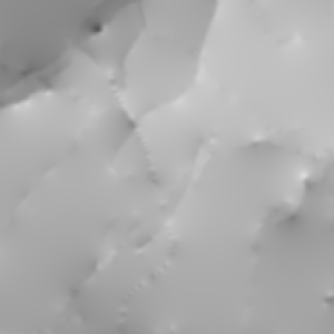
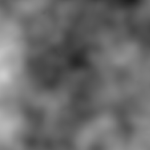
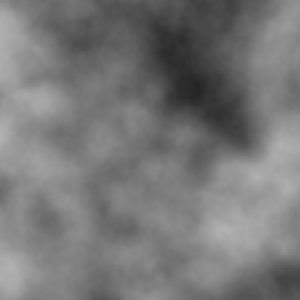
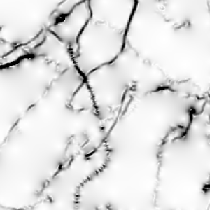
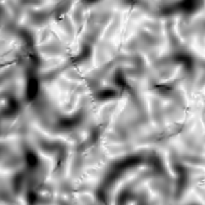
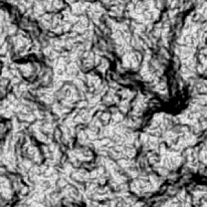
Figure 2: Simulated maps of the string signal with noise at $1$ arcminute resolution, on a field of view of $\tau^{\prime}=1.4^{\circ}$. The top left panel represents the test simulation of the string signal. The top middle and top right panels represent the combinations of this string signal simulation for a string tension $\rho=2\times 10^{-7}$ in the noise conditions PA$-$IN and SA$-$tSZ respectively. The bottom panels represent corresponding maps of the magnitude of gradient.

Our denoising approach is based on explicitly describing the statistical properties of the string signal on small angular scales. We need precise simulations of the string signal on planar patches for both training and validation of our method. We use $2$ simulations of the string signal borrowed from the full set of $84$ simulations produced by (Fraisse et al., 2008). The first simulation of the string signal is used as training data for fitting the prior probability distributions for the coefficients of the wavelet decomposition of the signal $s$, while the second is reserved for testing the algorithm. In the four noise conditions considered (PA$-$IN, PA$+$IN, SA$-$tSZ, or SA$+$tSZ), this test string signal simulations is combined with $100$ independent realizations of the noise in order to produce multiple test simulations.

The simulations are defined on planar patches of size $\tau\times\tau$ for a field of view defined by an angular opening $\tau=7.2^{\circ}$. The finite size of the patch induces a discretization of the spatial frequencies below the band limit $B$: $\textbf{\em k}=(2\pi/\tau)\textbf{\em p}=50\textbf{\em p}$ with $\textbf{\em p}=(p_{x},p_{y})$ and for integer values $p_{x}$ and $p_{y}$ with $-L\leq p_{x},p_{y}<L$ with $L=\tau B/2\pi=B/50$. The original maps are sampled on grids with $2L\times 2L$ uniformly sampled points $\textbf{\em x}_{i}$ with $1\leq i\leq 4L^{2}$ for $L=512$. The corresponding pixels thus have an angular size around $0.42^{\prime}$. The corresponding band limit on $k_{x}$ and $k_{y}$ thus reads $B\simeq 2.5\times 10^{4}$.

The astrophysical and instrumental components of the noise are modeled as statistically isotropic Gaussian noise on a planar patch with the appropriate power spectra. We consider instrumental noise with a standard deviation of $1\mu K$. For each noise component, a simulation may easily be produced by taking the Fourier transform of Gaussian white noise, renormalizing each Fourier frequency value by the square root of the corresponding power spectrum, and inverting the Fourier transform (Rocha et al., 2005). In each noise condition considered, an overall noise simulation is obtained by simple superposition of the required independent components simulated. The power spectrum of the noise $P^{n}(k)$ is the sum of the individual spectra.

We also include the effect of the experimental beam of a typical arcminute experiment in the training string signal simulation, as well as in all test simulations for each noise condition considered. We simply model this effect by convolution of the string signal and astrophysical noise components with a Gaussian kernel with a full width at half maximum (FWHM) of $1$ arcminute. This corresponds to a Gaussian tapering of angular frequencies with a FWHM of $2\times 10^{4}$, which effectively limits the angular frequencies not far above $B\simeq 10^{4}$. Hence the power spectrum $P^{s}(k,\rho)$ of the string signal in relation (3) and the power spectrum of the astrophysical noise components are multiplied by the square modulus of the Fourier transform of the experimental beam. The corresponding power spectra of the string signal and of the noise in each noise condition considered are respectively denoted as $\tilde{P}^{s}(k,\rho)$ and $\tilde{P}^{n}(k)$.

For illustration, Figure 2 represents simulated maps of the string signal and noise at the resolution considered, as well as corresponding maps of the magnitude of gradient. For visualization purposes, we show only one fifth of the total field of view, corresponding to an angular opening $\tau^{\prime}=1.4^{\circ}$. At a tension $\rho=2\times 10^{-7}$, with noise only including the primary CMB anisotropies, the strings are not visible by eye in the original map itself, while part of the network appears in the map of the magnitude of gradient. This illustrates the natural enhancement of high frequency features such as temperature steps by the gradient operator. At the same string tension, the presence of the secondary anisotropies adds noise at the highest angular frequencies and the strings are not visible by eye anymore in either the original map or the map of the magnitude of gradient, already when the thermal SZ effect is discarded.

3 Wavelets and Signal Sparsity

In this section, we firstly describe the steerable wavelet transform and reformulate the denoising problem in the wavelet domain. We then detail the probability distributions that we use to describe the marginal statistics of the wavelet coefficients of string signal and the noise.

3.1 Steerable wavelets

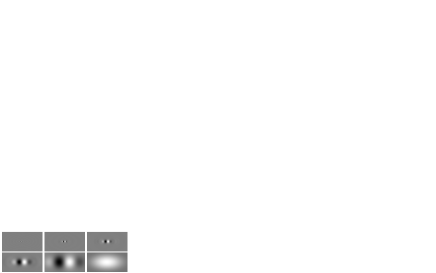
Figure 3: Steerable Pyramid wavelets with $N=6$ basis orientations, centered at the origin of the plane. From top left to bottom right, the highpass filter $\gamma_{h}$, the wavelets $\gamma_{q,j}$ with orientation $\chi_{N}=\pi$ (i.e. $q=N$) for the spatial scales $j=1$ to $j=4$, and the lowpass filter $\gamma_{l}$.

Wavelet transforms have become widely used in data analysis and image processing in recent years, and have found numerous applications in astrophysics (Hobson et al., 1999; Barreiro & Hobson, 2001; Starck et al., 2006a). In general, a particular transform will be useful for signal modeling and denoising if the properties of the signal of interest are easier to describe, or more distinct from the noise process, in the transform domain than in the original domain. The cosmic string signal is characterized by localized, oriented edge-like discontinuities. This motivates the use of a transform that is well adapted for representing localized oriented features.

Standard orthogonal wavelets are well localized, but are not well suited for arbitrarily oriented features as they have strong bias for horizontal and vertical orientations due to their tensor product construction. Instead, in this paper we use a steerable wavelet transform. The transform is parametrized by a number of orientations $N$ and spatial scales $J$. The output of the transform is given by the convolution of the original signal $f$ with a set of filters at different scales. These filters are formed by scaling and rotating a single, “mother” wavelet $\gamma(\textbf{\em x})$. For the discrete numerical transform, the rotation is sampled at $N$ equally spaced angles $\chi_{q}=q\pi/N$ for integer $q$ with $1\leq q\leq N$. The scalings are sampled dyadically, i.e. as $2^{-j}$ for integer $j$ with $1\leq j\leq J$. The transform output at spatial scale $j$ and orientation $q$ is given by $f\star\gamma_{q,j}$ where $\gamma_{q,j}(x)$ is given by rotating $\gamma$ by $\chi_{q}$ and scaling by $2^{-j}$.

In order to ensure the invertibility of the transform, it is also necessary to include residual highpass and lowpass bands, generated by filters $\gamma_{h}$ and $\gamma_{l}$ respectively. The output of the complete steerable wavelet transform then includes a highpass band, $J$ sets of $N$ oriented bandpass bands, and the lowpass band. Invertibility of the transform is important for our work, as we are interested in reconstructing the string map which resides in the image domain.

We adopt the notation $\textbf{\em W}^{f}$ to denote the full vector of wavelet coefficients for a given input signal $f$, where we have implicitly vectorized and concatenated the subbands corresponding to different scales and orientations. We will write $W^{f}_{I}$ to specify individual coefficients, where $I$ is a multi-index specifying the scale, orientation and spatial location of the coefficient. We will denote by $R$ the inverse wavelet transform operator, so that

$$f(\textbf{\em x})=\left[R\textbf{\em W}^{f}\right](\textbf{\em x})$$ (6)

In this work, we use a particular implementation known as the Steerable Pyramid (Simoncelli et al., 1992). We use the transform with $N=6$ orientations and $J=4$ spatial scales. The corresponding wavelet filters are shown in Figure 3 for orientation $\chi_{N}=\pi$. In particular, the filters that we employ have odd symmetry, which is especially appropriate for representing the edge-like discontinuities present in the string signal.

3.2 Problem reformulation in wavelet domain

\psfrag{-1.3e+06}{$-1.3\times 10^{6}$}\psfrag{1.3e+06}{$1.3\times 10^{6}$}\psfrag{-1.4e+07}{$-1.4\times 10^{7}$}\psfrag{1.4e+07}{$1.4\times 10^{7}$}\psfrag{-9.5e+07}{$-9.5\times 10^{7}$}\psfrag{9.5e+07}{$9.5\times 10^{7}$}\psfrag{-5.1e+08}{$-5.1\times 10^{8}$}\psfrag{5.1e+08}{$5.1\times 10^{8}$}\psfrag{-3.7e+05}{$-3.7\times 10^{5}$}\psfrag{3.7e+05}{$3.7\times 10^{5}$}\psfrag{-2.1e+10}{$-2.1\times 10^{10}$}\psfrag{2.1e+10}{$2.1\times 10^{10}$}\psfrag{-1.3e+06}{$-1.3\times 10^{6}$}\psfrag{1.3e+06}{$1.3\times 10^{6}$}\psfrag{-1.4e+07}{$-1.4\times 10^{7}$}\psfrag{1.4e+07}{$1.4\times 10^{7}$}\psfrag{-9.5e+07}{$-9.5\times 10^{7}$}\psfrag{9.5e+07}{$9.5\times 10^{7}$}\psfrag{-5.1e+08}{$-5.1\times 10^{8}$}\psfrag{5.1e+08}{$5.1\times 10^{8}$}\psfrag{-3.7e+05}{$-3.7\times 10^{5}$}\psfrag{3.7e+05}{$3.7\times 10^{5}$}\psfrag{-2.1e+10}{$-2.1\times 10^{10}$}\psfrag{2.1e+10}{$2.1\times 10^{10}$}\psfrag{-2}{-2}\psfrag{-3}{-3}\psfrag{-4}{-4}\includegraphics[width=142.26378pt]{figures/figure4_s2_logprobfig-hp}

\psfrag{-1.3e+06}{$-1.3\times 10^{6}$}\psfrag{1.3e+06}{$1.3\times 10^{6}$}\psfrag{-1.4e+07}{$-1.4\times 10^{7}$}\psfrag{1.4e+07}{$1.4\times 10^{7}$}\psfrag{-9.5e+07}{$-9.5\times 10^{7}$}\psfrag{9.5e+07}{$9.5\times 10^{7}$}\psfrag{-5.1e+08}{$-5.1\times 10^{8}$}\psfrag{5.1e+08}{$5.1\times 10^{8}$}\psfrag{-3.7e+05}{$-3.7\times 10^{5}$}\psfrag{3.7e+05}{$3.7\times 10^{5}$}\psfrag{-2.1e+10}{$-2.1\times 10^{10}$}\psfrag{2.1e+10}{$2.1\times 10^{10}$}\psfrag{-1.3e+06}{$-1.3\times 10^{6}$}\psfrag{1.3e+06}{$1.3\times 10^{6}$}\psfrag{-1.4e+07}{$-1.4\times 10^{7}$}\psfrag{1.4e+07}{$1.4\times 10^{7}$}\psfrag{-9.5e+07}{$-9.5\times 10^{7}$}\psfrag{9.5e+07}{$9.5\times 10^{7}$}\psfrag{-5.1e+08}{$-5.1\times 10^{8}$}\psfrag{5.1e+08}{$5.1\times 10^{8}$}\psfrag{-3.7e+05}{$-3.7\times 10^{5}$}\psfrag{3.7e+05}{$3.7\times 10^{5}$}\psfrag{-2.1e+10}{$-2.1\times 10^{10}$}\psfrag{2.1e+10}{$2.1\times 10^{10}$}\psfrag{-2}{-2}\psfrag{-3}{-3}\psfrag{-4}{-4}\includegraphics[width=142.26378pt]{figures/figure4_s2_logprobfig-1}

\psfrag{-1.3e+06}{$-1.3\times 10^{6}$}\psfrag{1.3e+06}{$1.3\times 10^{6}$}\psfrag{-1.4e+07}{$-1.4\times 10^{7}$}\psfrag{1.4e+07}{$1.4\times 10^{7}$}\psfrag{-9.5e+07}{$-9.5\times 10^{7}$}\psfrag{9.5e+07}{$9.5\times 10^{7}$}\psfrag{-5.1e+08}{$-5.1\times 10^{8}$}\psfrag{5.1e+08}{$5.1\times 10^{8}$}\psfrag{-3.7e+05}{$-3.7\times 10^{5}$}\psfrag{3.7e+05}{$3.7\times 10^{5}$}\psfrag{-2.1e+10}{$-2.1\times 10^{10}$}\psfrag{2.1e+10}{$2.1\times 10^{10}$}\psfrag{-1.3e+06}{$-1.3\times 10^{6}$}\psfrag{1.3e+06}{$1.3\times 10^{6}$}\psfrag{-1.4e+07}{$-1.4\times 10^{7}$}\psfrag{1.4e+07}{$1.4\times 10^{7}$}\psfrag{-9.5e+07}{$-9.5\times 10^{7}$}\psfrag{9.5e+07}{$9.5\times 10^{7}$}\psfrag{-5.1e+08}{$-5.1\times 10^{8}$}\psfrag{5.1e+08}{$5.1\times 10^{8}$}\psfrag{-3.7e+05}{$-3.7\times 10^{5}$}\psfrag{3.7e+05}{$3.7\times 10^{5}$}\psfrag{-2.1e+10}{$-2.1\times 10^{10}$}\psfrag{2.1e+10}{$2.1\times 10^{10}$}\psfrag{-2}{-2}\psfrag{-3}{-3}\psfrag{-4}{-4}\includegraphics[width=142.26378pt]{figures/figure4_s2_logprobfig-2}

\psfrag{-1.3e+06}{$-1.3\times 10^{6}$}\psfrag{1.3e+06}{$1.3\times 10^{6}$}\psfrag{-1.4e+07}{$-1.4\times 10^{7}$}\psfrag{1.4e+07}{$1.4\times 10^{7}$}\psfrag{-9.5e+07}{$-9.5\times 10^{7}$}\psfrag{9.5e+07}{$9.5\times 10^{7}$}\psfrag{-5.1e+08}{$-5.1\times 10^{8}$}\psfrag{5.1e+08}{$5.1\times 10^{8}$}\psfrag{-3.7e+05}{$-3.7\times 10^{5}$}\psfrag{3.7e+05}{$3.7\times 10^{5}$}\psfrag{-2.1e+10}{$-2.1\times 10^{10}$}\psfrag{2.1e+10}{$2.1\times 10^{10}$}\psfrag{-1.3e+06}{$-1.3\times 10^{6}$}\psfrag{1.3e+06}{$1.3\times 10^{6}$}\psfrag{-1.4e+07}{$-1.4\times 10^{7}$}\psfrag{1.4e+07}{$1.4\times 10^{7}$}\psfrag{-9.5e+07}{$-9.5\times 10^{7}$}\psfrag{9.5e+07}{$9.5\times 10^{7}$}\psfrag{-5.1e+08}{$-5.1\times 10^{8}$}\psfrag{5.1e+08}{$5.1\times 10^{8}$}\psfrag{-3.7e+05}{$-3.7\times 10^{5}$}\psfrag{3.7e+05}{$3.7\times 10^{5}$}\psfrag{-2.1e+10}{$-2.1\times 10^{10}$}\psfrag{2.1e+10}{$2.1\times 10^{10}$}\psfrag{-2}{-2}\psfrag{-3}{-3}\psfrag{-4}{-4}\includegraphics[width=142.26378pt]{figures/figure4_s2_logprobfig-3}

\psfrag{-1.3e+06}{$-1.3\times 10^{6}$}\psfrag{1.3e+06}{$1.3\times 10^{6}$}\psfrag{-1.4e+07}{$-1.4\times 10^{7}$}\psfrag{1.4e+07}{$1.4\times 10^{7}$}\psfrag{-9.5e+07}{$-9.5\times 10^{7}$}\psfrag{9.5e+07}{$9.5\times 10^{7}$}\psfrag{-5.1e+08}{$-5.1\times 10^{8}$}\psfrag{5.1e+08}{$5.1\times 10^{8}$}\psfrag{-3.7e+05}{$-3.7\times 10^{5}$}\psfrag{3.7e+05}{$3.7\times 10^{5}$}\psfrag{-2.1e+10}{$-2.1\times 10^{10}$}\psfrag{2.1e+10}{$2.1\times 10^{10}$}\psfrag{-1.3e+06}{$-1.3\times 10^{6}$}\psfrag{1.3e+06}{$1.3\times 10^{6}$}\psfrag{-1.4e+07}{$-1.4\times 10^{7}$}\psfrag{1.4e+07}{$1.4\times 10^{7}$}\psfrag{-9.5e+07}{$-9.5\times 10^{7}$}\psfrag{9.5e+07}{$9.5\times 10^{7}$}\psfrag{-5.1e+08}{$-5.1\times 10^{8}$}\psfrag{5.1e+08}{$5.1\times 10^{8}$}\psfrag{-3.7e+05}{$-3.7\times 10^{5}$}\psfrag{3.7e+05}{$3.7\times 10^{5}$}\psfrag{-2.1e+10}{$-2.1\times 10^{10}$}\psfrag{2.1e+10}{$2.1\times 10^{10}$}\psfrag{-2}{-2}\psfrag{-3}{-3}\psfrag{-4}{-4}\includegraphics[width=142.26378pt]{figures/figure4_s2_logprobfig-4}

\psfrag{-1.3e+06}{$-1.3\times 10^{6}$}\psfrag{1.3e+06}{$1.3\times 10^{6}$}\psfrag{-1.4e+07}{$-1.4\times 10^{7}$}\psfrag{1.4e+07}{$1.4\times 10^{7}$}\psfrag{-9.5e+07}{$-9.5\times 10^{7}$}\psfrag{9.5e+07}{$9.5\times 10^{7}$}\psfrag{-5.1e+08}{$-5.1\times 10^{8}$}\psfrag{5.1e+08}{$5.1\times 10^{8}$}\psfrag{-3.7e+05}{$-3.7\times 10^{5}$}\psfrag{3.7e+05}{$3.7\times 10^{5}$}\psfrag{-2.1e+10}{$-2.1\times 10^{10}$}\psfrag{2.1e+10}{$2.1\times 10^{10}$}\psfrag{-1.3e+06}{$-1.3\times 10^{6}$}\psfrag{1.3e+06}{$1.3\times 10^{6}$}\psfrag{-1.4e+07}{$-1.4\times 10^{7}$}\psfrag{1.4e+07}{$1.4\times 10^{7}$}\psfrag{-9.5e+07}{$-9.5\times 10^{7}$}\psfrag{9.5e+07}{$9.5\times 10^{7}$}\psfrag{-5.1e+08}{$-5.1\times 10^{8}$}\psfrag{5.1e+08}{$5.1\times 10^{8}$}\psfrag{-3.7e+05}{$-3.7\times 10^{5}$}\psfrag{3.7e+05}{$3.7\times 10^{5}$}\psfrag{-2.1e+10}{$-2.1\times 10^{10}$}\psfrag{2.1e+10}{$2.1\times 10^{10}$}\psfrag{-2}{-2}\psfrag{-3}{-3}\psfrag{-4}{-4}\includegraphics[width=142.26378pt]{figures/figure4_s2_logprobfig-lp}

Figure 4: Logarithm of the modeled prior GGD’s $\pi_{b}$ for the wavelet coefficients $W_{I}^{s}$ of a string signal (red solid curves), computed using $N=6$ orientations and $J=4$ spatial scales, superimposed on the histograms of the corresponding coefficients from the training simulation (black dashed curves) for $b=\{h,j,l\}$ and $1\leq j\leq J=4$. From top left to bottom right, the coefficients associated with the highpass filter $\gamma_{h}$, with the wavelets $\gamma_{q,j}$ for the spatial scales $j=1$ to $j=4$, and with the lowpass filter $\gamma_{l}$.

$b$	$u_{b}$	$v_{b}$	$\sigma_{b}^{s}(\rho=1)$	$\kappa_{b}^{s}$	$\sigma_{b}^{n}$ (PA$-$IN)	$\sigma_{b}^{n}$(SA$-$tSZ)	$\sigma_{b}^{n}$(SA$+$tSZ)
$h$	$3.8\times 10^{3}$	$0.41$	$1.2\times 10^{5}$	$47$	$4.7\times 10^{-4}$	$8.6\times 10^{-2}$	$0.16$
$j=1$	$1.6\times 10^{4}$	$0.42$	$4.1\times 10^{5}$	$42$	$4.5\times 10^{-3}$	$0.26$	$0.56$
$j=2$	$3.8\times 10^{5}$	$0.49$	$4.5\times 10^{6}$	$26$	$0.55$	$2.3$	$5.4$
$j=3$	$7.2\times 10^{6}$	$0.63$	$3.1\times 10^{7}$	$14$	$32$	$35$	$44$
$j=4$	$9.9\times 10^{7}$	$0.88$	$1.8\times 10^{8}$	$7.3$	$4.9\times 10^{2}$	$4.9\times 10^{2}$	$5.1\times 10^{2}$
$l$	$9.8\times 10^{9}$	$1.5$	$8.3\times 10^{9}$	$3.7$	$2.5\times 10^{4}$	$2.5\times 10^{4}$	$2.5\times 10^{4}$

Table 1: Parameters for the modeled prior GGD’s $\pi_{b}$ and noise Gaussian distributions $g_{b}$ for the spatial scales $b=\{h,j,l\}$ and $1\leq j\leq J=4$. The first column identifies the spatial scale $b$. The next four columns identify the parameters $u_{b}$ and $v_{b}$, and the corresponding standard deviations $\sigma_{b}^{s}$ at $\rho=1$ and kurtoses $\kappa_{b}^{s}$ for the prior GGD’s. The last three columns identify the standard deviations $\sigma_{b}^{n}$ for the noise distributions in the noise conditions PA$-$IN, SA$-$tSZ, and SA$+$tSZ. All values are given with two significant figures.

By linearity of the wavelet transform, the coefficients of the observed signal in relation (4) are a sum of the wavelet coefficients for the string signal and the Gaussian CMB noise, i.e.

$$W_{I}^{f}=W_{I}^{s}+W_{I}^{n}.$$ (7)

The overall denoising algorithm will proceed by computing the wavelet decomposition of the observed signal, estimating the coefficients corresponding to the string signal, and finally inverting the wavelet transform. Our Bayesian estimator requires knowledge of probability distributions describing the behaviour of both the string signal and the noise. As we shall see later, part of our denoising procedure will assume independence of the coefficients for different $I$, allowing it to use a model for the marginal probability distribution of the coefficients.

Notice that by statistical isotropy of both the signal and noise processes, the probability distributions of the wavelet coefficients for different spatial scales $j$ do not depend on position or orientation. For notational convenience we introduce a generalized spatial scale $b\in\{l,j,h\}$ for $1\leq j\leq J$. The above comment implies that the signal and noise distributions depend only on $b$. The distribution for the string coefficients will depend on the string tension $\rho$. We write this as the conditional probability $\pi_{b}(W_{I}^{s}|\rho)$. The noise coefficient distribution will be denoted $g_{b}(W^{n}_{I})$.

3.3 String signal distribution

The morphology of the string signal should give rise to sparse distribution of its wavelet coefficients, i.e. many coefficients are close to zero with a small number of large magnitude coefficients near the temperature steps. We observe this behaviour in our training simulation. The sparse wavelet coefficients can be successfully modeled by a class of probability distributions known as the Generalized Gaussian Distributions (GGD).

We thus use a GGD to model the prior distributions $\pi_{b}$:

$$\pi_{b}\left(x|\rho\right)=\frac{v_{b}}{2\left(\rho u_{b}\right)\Gamma\left(v_{b}^{-1}\right)}\exp\left[-\Big{|}\frac{x}{\rho u_{b}}\Big{|}^{v_{b}}\right],$$ (8)

where $\Gamma$ is the Gamma function, and where $v_{b}$ and $\rho u_{b}$ are respectively called shape parameters and scale parameters. These distributions all have zero statistical means as the signal itself is defined in relation (4) as a zero mean perturbation.

Let us acknowledge that GGD’s have been used previously to model wavelet coefficients for various image processing applications including denoising (Simoncelli & Adelson, 1996; Moulin & Liu, 1999), deconvolution (Belge et al., 2000), and coding (Antonini et al., 1992; Mallat, 1998).

The shape parameters $v_{b}$ can be considered as a continuous measure of the sparsity of the underlying distribution. Setting $v_{b}=2$ recovers the Gaussian distribution, which is non-sparse. Letting $v_{b}$ approach $0$ yields very peaked probability distributions with heavy tails relative to Gaussian distributions, i.e. very sparse distributions. These parameters determine the kurtoses $\kappa_{b}^{s}$, i.e. the ratio of the fourth central moment to the square of the variance (second central moment), by

$$\kappa_{b}^{s}=\frac{\Gamma\left(5v_{b}^{-1}\right)\Gamma\left(v_{b}^{-1}\right)}{\left[\Gamma\left(3v_{b}^{-1}\right)\right]^{2}}.$$ (9)

The scale parameters $\rho u_{b}$ are linearly proportional to the standard deviations $\sigma_{b}^{s}$ of the distributions. The corresponding variances reflect the power spectrum (3) of the string signal in the range of spatial frequencies $k$ probed by the filter at scale $b$, and thus also scale as $\rho^{2}$:

$$\left(\sigma_{b}^{s}\right)^{2}=\rho^{2}\frac{\Gamma\left(3v_{b}^{-1}\right)}{\Gamma\left(v_{b}^{-1}\right)}u_{b}^{2}.$$ (10)

The parameters $v_{b}$ and $u_{b}$ are estimated by a moment method from the wavelet decomposition of the training simulation of the string signal for a given string tension $\rho$. For each spatial scale, the sample variance and kurtosis are calculated, then equations (9) and (10) are solved numerically to obtain $v_{b}$ and $u_{b}$.

Figure 4 shows the modeled prior GGD’s $\pi_{b}$ for the coefficients of the string signal with the steerable wavelet $\gamma$ with $N=6$ orientations and $J=4$ spatial scales (see Figure 3). The GGD’s are superimposed on the histograms of the corresponding coefficients from the training simulation. As the distributions for coefficients of different orientations at the same spatial scale will be identical by statistical isotropy, the corresponding histograms are produced by aggregating the coefficients over all $6$ orientations. Qualitatively, we see that the prior distributions $\pi_{b}$ are well modeled by GGD’s, which justifies our choice of parameters $N$ and $J$.

The estimated values of the parameters $u_{b}$ and $v_{b}$, and corresponding standard deviations $\sigma_{b}^{s}$ and kurtoses $\kappa_{b}^{s}$ are reported in the columns two to five of Table 1. Notice that the shape parameters measured for the highpass band ($b=h$) and for the four bandpass bands ($j=1$ to $j=4$) are significantly lower than $2$, corresponding to very sparse distributions. The larger value for the shape parameter for the lowpass band justifies our choice of $J=4$ for the maximal spatial scale. At the scales accounted for by the lowpass filter, the signal coefficients are not significantly non-Gaussian and will not be very sparsely distributed. The reconstruction of temperature steps therefore does not strongly rely on those scales.

3.4 Noise distribution

The Gaussian probability distributions $g_{b}$ for the noise coefficients $W_{I}^{n}$ are defined as:

$$g_{b}\left(x\right)=\frac{1}{\sigma_{b}^{n}\sqrt{2\pi}}\exp\left[-\frac{1}{2}\left(\frac{x}{\sigma_{b}^{n}}\right)^{2}\right].$$ (11)

These distributions are all zero mean, as the noise itself is defined in relation (4) as a zero mean perturbation. For each of the noise conditions PA$-$IN, PA$+$IN, SA$-$tSZ, or SA$+$tSZ, the variances $(\sigma_{b}^{n})^{2}$ can be inferred from the power spectrum $\tilde{P}^{n}(k)$ of the noise at $1$ arcminute resolution in the range of spatial frequencies $k$ probed by the wavelets at the different spatial scales:

$$\left(\sigma_{b}^{n}\right)^{2}=\frac{1}{\tau^{2}}\sum_{\{p_{x,}p_{y}\}=-L}^{L-1}|\widehat{\gamma}_{G}\left(\textbf{\em k}\right)|^{2}\tilde{P}^{n}\left(k\right).$$ (12)

In this relation, the multi-index value $G$ reads as $G=(q,j)$ with $1\leq q\leq N$ and $1\leq j\leq J$ for the oriented wavelet coefficients, $G=l$ for the lowpass coefficients, and $G=h$ for the highpass coefficients. Notice that due to the rotational invariance of the noise power spectrum, the variances calculated in equation (12) do not depend on the orientation $q$. The values of the standard deviations $\sigma_{b}^{n}$ for the noise conditions PA$-$IN, SA$-$tSZ, and SA$+$tSZ are listed in the last three columns of Table 1.

4 Bayesian denoising

In this section, we define in detail our wavelet domain Bayesian denoising (WDBD) algorithm. We define an overall Bayesian least squares estimator as an average of estimation functions evaluated at each value of the unknown string tension, weighted by the posterior probability distribution for the string tension. We then discuss Wiener filtering as a standard alternative to our WDBD algorithm.

4.1 Bayesian least squares

In a Bayesian approach the signal coefficients $\textbf{\em W}^{s}$ are estimated from their posterior probability distribution given the coefficients of the observed signal $\textbf{\em W}^{f}$: $p(\textbf{\em W}^{s}|\textbf{\em W}^{f})$. Under our general assumption that the standard cosmological parameters are fixed at their concordance values while the string tension remains undetermined this posterior probability distribution reads as

$$p\left(\textbf{\em W}^{s}|\textbf{\em W}^{f}\right)=\int\textnormal{d}\rho\,p\left(\rho|\textbf{\em W}^{f}\right)\,p\left(\textbf{\em W}^{s}|\textbf{\em W}^{f},\rho\right),$$ (13)

where $p(\rho|\textbf{\em W}^{f})$ is the posterior probability distribution function for $\rho$ given $\textbf{\em W}^{f}$ and $p\left(\textbf{\em W}^{s}|\textbf{\em W}^{f},\rho\right)$ is the posterior probability distribution function for $\textbf{\em W}^{s}$ given $\textbf{\em W}^{f}$ and $\rho$.

Several possible methods for selecting an appropriate estimate given the posterior probability distribution are possible. Maximizing this distribution leads to the maximum a posteriori (MAP) estimate. Other approaches may consist of minimizing some expected cost function. We employ the well known Bayesian least squares estimate which minimizes a quadratic cost function. This estimate is given by the expectation value of the posterior probability distribution. Using relation (13) and the linearity of the expectation value, our estimator may be written as

$$\overline{\textbf{\em W}^{s}}=E\left[\textbf{\em W}^{s}|\textbf{\em W}^{f}\right]=\int\textnormal{d}\rho\,p\left(\rho|\textbf{\em W}^{f}\right)\,\overline{\textbf{\em W}^{s}}\left(\rho\right),$$ (14)

with

$$\overline{\textbf{\em W}^{s}}\left(\rho\right)=E\left[\textbf{\em W}^{s}|\textbf{\em W}^{f},\rho\right]\\ =\int\textnormal{d}\textbf{\em W}^{s}\,\textbf{\em W}^{s}\,p\left(\textbf{\em W}^{s}|\textbf{\em W}^{f},\rho\right).$$ (15)

This estimation of the signal coefficients is thus given by the mean of the estimations for different string tensions, weighted by posterior probability distribution for $\rho$ given the observed signal.

4.2 Estimation functions

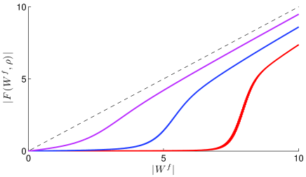
Figure 5: Bayesian least squares estimation functions $F(\cdot,\rho)$ depending on observed coefficient $W_{I}^{f}$ at a non-specified spatial scale and for various string tensions $\rho$. We consider a shape parameter $v=0.5$ and various scale parameters $\rho u$ identifying various standard deviations $\sigma^{s}$ of the coefficients of the string signal, all for a unit standard deviation of the noise $\sigma^{n}=1$. The black dashed curve shows the limit $\rho\rightarrow\infty$, where the estimation function is the identity function. The upper solid curve (magenta) relates to $\rho u=0.1$, i.e. $\sigma^{s}\simeq 1.1$, the middle solid curve (blue) relates to $\rho u=1.5\times 10^{-2}$, i.e. $\sigma^{s}=0.16$, while the lower solid curve (red) relates to $\rho u=5\times 10^{-3}$, i.e. $\sigma^{s}=5.5\times 10^{-2}$.

We concentrate firstly on computation of $\overline{\textbf{\em W}^{s}}\left(\rho\right)$ from equation (15). Notice that the coefficients of the wavelet decomposition of the signal and noise are correlated at different orientations, spatial scales and positions. Formally one should construct probability distributions accounting for these correlations. However, this would require computing expectations in a space with dimension equal to the number of coefficients of the wavelet decomposition. In this perspective, approaches accounting for correlations of the string signal developed in the framework of maximum entropy methods (MEM) (Gull & Skilling, 1999; Maisinger et al., 1999) might be considered. However such methods assume entropic prior models and are therefore not directly compatible with our prior model in terms of GGD’s for the coefficients of the string signal.

Accordingly, we employ the simplifying assumption that the wavelet coefficients for both the signal and noise for different values of $I$ are independent, after conditioning on the string tension $\rho$. Under this assumption, the integral in expression (15) may be factorized, and each coefficient $\overline{W_{I}^{s}}$ of the estimate depends only on the corresponding observed value $W_{I}^{f}$. To simplify the notation in the following, we write $x=W_{I}^{s}$ and $y=W_{I}^{f}$ to refer to the individual pure string coefficients and observed signal coefficients. We shall see that the resulting estimator will also depend on the spatial scale $b$.

Each coefficient $x$ may then be estimated as a function of the corresponding observed value $y$. By Bayes’ theorem we have that $p(x|y,\rho)\propto p(y|x,\rho)p(x|\rho)$. The probability $p(x|\rho)$ is exactly the marginal probability for each coefficient, which we have modeled as the GGD $\pi_{b}$. Conditioned on the signal $x$, the probability of observing $y$ is equal to the probability of the noise coefficient being equal to exactly $y-x$. Thus $p(y|x,\rho)$ is equal to $g_{b}(y-x)$. We thus have the posterior probability distribution

$$p(x|y,\rho)=C^{-1}\mbox{ }g_{b}(y-x)\pi_{b}(x|\rho)$$ (16)

and our Bayesian estimator at spatial scale $b$ is

$$E[x|y,\rho]=C^{-1}\int xg_{b}(y-x)\pi_{b}(x|\rho)dx$$ (17)

with normalization $C=\int g_{b}(y-x)\pi_{b}(x|\rho)dx$. This expression depends only on the observed coefficient $y$, the tension $\rho$ and the scale $b$. This defines the estimation function $F_{b}(y,\rho)=E[x|y,\rho]$. Returning to our original notation, the estimated string coefficients are given by evaluation of the estimation function at each scale, i.e.

$$\overline{W_{I}^{s}}\left(\rho\right)=F_{b}\left(W_{I}^{f},\rho\right).$$ (18)

In practice, these estimation functions are computed by numerical integration and tabulated for the different spatial scales $b$ and the required range of string tensions. Figure 5 shows generic shapes of estimation functions $F(\cdot,\rho)$ at a non-specified spatial scale and for various string tensions $\rho$. For the sake of illustration, we consider a shape parameter $v=0.5$ and various scale parameters $\rho u$ identifying various standard deviations $\sigma^{s}$ of the coefficients of the string signal, all for a unit standard deviation of the noise $\sigma^{n}=1$. Notice that the estimation functions are odd, and always shrink the magnitude of their input, i.e. $|F(W_{I}^{f},\rho)|<|W_{I}^{f}|$. Qualitatively, they behave as a smooth thresholding operation on the observed coefficient $|W_{I}^{f}|$, sending small magnitude coefficients closer to zero while preserving large magnitude coefficients. For small string tensions, the noise dominates the signal and the effective thresholding is more severe, while for large string tensions the noise becomes negligible and $F_{b}(\cdot,\rho)$ reduces to the identity.

In the particular case of Gaussian signal coefficients ($v=2$), the Bayesian least squares estimation is equivalent to simple Wiener filtering of the coefficients. Also notice that in the case of Laplacian signal coefficients ($v=1$), the estimation function for MAP estimation would reduce to the well known soft-thresholding operation (Moulin & Liu, 1999). By definition, this specific instance of thresholding operation sends to zero coefficients with an absolute value below some threshold, and reduces the absolute value of coefficients above the threshold by the value of the threshold itself.

4.3 Posterior string tension distribution

By Bayes’ theorem, the posterior probability distribution function for $\rho$ given the observed signal $p(\rho|\textbf{\em W}^{f})$ is simply obtained from the likelihood $\mathcal{L}(\textbf{\em W}^{f}|\rho)$ and the prior probability distribution function $p(\rho)$ on $\rho$. For complete consistency, the likelihood should be calculated using the framework of the model established for the coefficients, based on relation (7) and on the prior GGD’s $\pi_{b}$. However, while this model by construction accounts for the non-Gaussianity, i.e. sparsity, of the string signal, it ignores the correlation between coefficients.

We have observed that a likelihood yielding a more precise localization of the string tension value can actually be obtained using a power spectral model. Such a model assumes both the string signal and the noise arise from statistically isotropic Gaussian random processes, such that their Fourier coefficients are independent Gaussian variables. This assumption relies on the idea that the characteristic temperature steps of the string signal are smoothed by projection on the non-local imaginary exponentials defining the Fourier basis. Under this model, as the string signal and noise are independent, the observed signal $f$ has a power spectrum

$$\tilde{P}\left(k,\rho\right)=\tilde{P}^{n}\left(k\right)+\tilde{P}^{s}\left(k,\rho\right),$$ (19)

In this setting the likelihood can be computed most easily in terms of the Fourier transform $\widehat{f}$ of the observed signal. Accounting for the complex value of the Fourier coefficients as well as for the symmetry $\widehat{f}(-\textbf{\em k})=\widehat{f}^{*}(\textbf{\em k})$ that holds for real signals $f(\textbf{\em x})$, this likelihood reads as:

$$\mathcal{L}\left(\widehat{f}|\rho\right)=\prod_{\{p_{x,}p_{y}\}=-L}^{L-1}\frac{1}{\sqrt{\pi\tilde{P}\left(k,\rho\right)}}\exp\left[-\frac{1}{2}\frac{|\widehat{f}\left(\textbf{\em k}\right)|^{2}}{\tilde{P}\left(k,\rho\right)}\right],$$ (20)

where $|\cdot|$ stands for the modulus of a complex variable. The posterior probability distribution function for $\rho$ given the observed signal thus reads as

$$p\left(\rho|\widehat{f}\right)=D^{-1}\mbox{ }p\left(\rho\right)\mathcal{L}\left(\widehat{f}|\rho\right)$$ (21)

with normalization $D=\int p(\rho)\mathcal{L}(\hat{f}|\rho)d\rho$. We take the prior $p(\rho)$ to be flat in an interval $\rho\in[0,\rho_{\mbox{{\scriptsize max}}}]$, with an upper bound $\rho_{\mbox{{\scriptsize max}}}$ large enough relative to the upper bound associated with the best experimental constraints (5): $\rho_{\mbox{{\scriptsize max}}}>\rho_{\mbox{{\scriptsize exp}}}$. In practice, $\mathcal{L}(\widehat{f}|\rho)$ decays so rapidly for large $\rho$ that the resulting posterior is not sensitive to the value $\rho_{\mbox{{\scriptsize max}}}$ provided that it is greater than the effective support of $\mathcal{L}(\widehat{f}|\rho)$.

We use this PSM posterior $p(\rho|\widehat{f})$ in the place of $p(\rho|\textbf{\em W}^{f})$ in equation (14). Each component of the string coefficient $\textbf{\em W}^{s}$ is thus estimated as

$$\overline{W^{s}_{I}}=\int p(\rho|\widehat{f})F_{b}(W^{f}_{I},\rho)d\rho.$$ (22)

In practice, this integral is computed numerically by sampling 20 values of $\rho$ chosen to cover the effective support of $p(\rho|\widehat{f})$.

The estimated string signal in the original image domain is then given by inverting the wavelet transform, i.e.

$$\overline{s}(\textbf{\em x})=\left[R\overline{\textbf{\em W}}^{s}\right](\textbf{\em x})$$ (23)

4.4 Alternative Wiener filtering

In order to obtain a more precise estimation of the posterior probability distribution function for $\rho$, we have explicitly set up a PSM assuming that the string signal arises from a statistically isotropic Gaussian random process, such that its Fourier coefficients are independent Gaussian variables, just as for the noise.

At each string tension allowed by $p(\rho|\widehat{f})$, one may now consider estimating the string signal $s$ from the observed signal $f$ simply using this Gaussianity assumption. In this case the Bayesian least squares estimate for a string tension $\rho$ reduces to Wiener filtering in the Fourier domain, so that:

$$\overline{\widehat{s}}\left(\textbf{\em k},\rho\right)=\frac{\tilde{P}^{s}\left(k,\rho\right)}{\tilde{P}^{n}\left(k\right)+\tilde{P}^{s}\left(k,\rho\right)}\widehat{f}\left(\textbf{\em k}\right).$$ (24)

Analogously to relation (22), the estimate of the string signal in the Fourier domain is

$$\overline{\widehat{s}}(\textbf{\em k})=\int p(\rho|\widehat{f})\overline{\widehat{s}}(\textbf{\em k},\rho)d\rho,$$ (25)

and the estimate in the image domain is recovered by inverting the Fourier transform.

Let us acknowledge the fact that this alternative Wiener filtering based procedure relies only on the knowledge of the power spectra of both the signal and noise, while our WDBD approach relies on a training simulation for an explicit modeling of the prior GGD’s for the coefficients of a wavelet decomposition of the string signal. However, from the theoretical point of view it is clear that the Wiener filtering approach, which disregards the non-Gaussianity of the signal to be recovered, will be less effective at identifying this signal than our WDBD procedure, which explicitly accounts for the corresponding sparsity. While the Gaussianity assumption is useful for estimating a single global parameter such as the string tension on the basis of a PSM, it is not optimal for the explicit reconstruction of the sparse features of the string network itself. This fact is illustrated in our analysis the algorithm performance in the next section.

5 Algorithm performance

In this section, we firstly define the WDBD performance criteria to be the signal-to-noise ratio, correlation coefficient, and kurtosis of the map of the magnitude of gradient of the string signal. We then study the algorithm performance in each noise condition, in comparison with Wiener filtering. We also examine a detectability threshold on the string tension based on on the PSM, and compare it with an eye visibility threshold for the WDBD algorithm.

5.1 WDBD performance criteria

As already emphasized, denoising may be used as a pre-processing step for other methods for cosmic string detection based on explicit edge detection (Jeong & Smoot, 2005; Lo & Wright, 2005; Amsel et al., 2007). The relative performance of such methods before and after denoising might be an effective criterion for evaluating the denoising performance itself. Here we evaluate the performance of WDBD independently of any further processing.

The overall denoising is effective for string mapping if the magnitude of gradient of the denoised signal closely resembles the magnitude of gradient of the true string signal. A simple qualitative measure of the denoising performance is given by whether the string network is visible in the magnitude of gradient of the denoised signal. We define the eye visibility threshold as the minimum string tension around which the overall denoising and mapping by the magnitude of the gradient begins to exhibit string features visible by eye. We will augment this qualitative assessment of the denoising performance with three quantitative measures, namely the signal-to-noise ratio, the correlation coefficient and the kurtosis of the magnitude of the gradient of the denoised string signal. The first two of these are computed with respect to the original known signal, while the kurtosis is computed only using the denoised signal. The kurtosis is known to be a good statistic for discriminating between models with and without cosmic strings (Moessner et al., 1994).

The signal-to-noise ratio is defined in terms of the magnitude of gradient $|\mathbf{\nabla}s|(\textbf{\em x})$ of the original string signal $s(\textbf{\em x})$ in relation (4), and of the magnitude of gradient $|\mathbf{\nabla}\overline{s}|(\textbf{\em x})$ of the denoised signal $\overline{s}(\textbf{\em x})$ in relation (23) as

$$\textnormal{SNR}^{(|\mathbf{\nabla}s|,|\mathbf{\nabla}\overline{s}|)}=-20\log_{10}\frac{\sigma^{(|\mathbf{\nabla}s|-|\mathbf{\nabla}\overline{s}|)}}{\sigma^{|\mathbf{\nabla}s|}},$$ (26)

where $\sigma^{(|\mathbf{\nabla}s|-|\mathbf{\nabla}\overline{s}|)}$ and $\sigma^{|\mathbf{\nabla}s|}$ respectively stand for the standard deviations of the discrepancy signal $|\mathbf{\nabla}s|-|\mathbf{\nabla}\overline{s}|$ and of the original signal $|\mathbf{\nabla}s|$. The standard deviations are estimated from the sample variances on the basis of the signal realizations concerned. With this definition, the $\textnormal{SNR}^{(|\mathbf{\nabla}s|,|\mathbf{\nabla}\overline{s}|)}\in\mathbb{R}$ is measured in decibels (dB). Large negative and positive values are respectively associated with large and small discrepancy signals relative to the original signal. An exact recovery of the string network would provide an infinite signal-to-noise ratio. We will consider that the denoising is effective in terms of signal-to-noise ratio for the values of $\rho$ where this statistic is larger after denoising than before, and positive.

The correlation coefficient is defined in terms of the magnitude of gradient of the original and denoised string signals as

$$r^{(|\mathbf{\nabla}s|,|\mathbf{\nabla}\overline{s}|)}=\frac{\textnormal{cov}^{(|\mathbf{\nabla}s|,|\mathbf{\nabla}\overline{s}|)}}{\sigma^{|\mathbf{\nabla}s|}\sigma^{|\mathbf{\nabla}\overline{s}|}},$$ (27)

where $\textnormal{cov}^{(|\mathbf{\nabla}s|,|\mathbf{\nabla}\overline{s}|)}$ stands for the covariance between $|\mathbf{\nabla}s|$ and $|\mathbf{\nabla}\overline{s}|$. This signal covariance is also estimated from the sample covariance on the basis of the signal realizations concerned. An exact recovery of the string network would provide a unit correlation coefficient. The null value corresponds to a reconstruction completely decorrelated from the original signal. We will consider that the denoising is effective in terms of correlation coefficient for the values of $\rho$ where this statistic is larger after denoising than before, and positive.

Analogously, kurtoses are estimated from the sample kurtoses on the basis of the signal realizations concerned. The estimated kurtosis of the magnitude of gradient of pure Gaussian noise is distributed around a mean value across all test simulations $\kappa^{|\mathbf{\nabla}n|}\simeq 3$, even though the magnitude of gradient itself is not Gaussian. At the arcminute resolution considered, the estimated kurtosis of the magnitude of gradient of a pure string signal is much higher than the value associated with pure noise, with a value around $\kappa^{|\mathbf{\nabla}s|}\simeq 32$ in the training simulation. The estimated kurtosis of the magnitude of gradient of a string signal with noise before denoising naturally lies in the interval $[\kappa^{|\mathbf{\nabla}n|},\kappa^{|\mathbf{\nabla}s|}]$, for any value of the string tension $\rho$. Its mean value $\kappa^{|\mathbf{\nabla}f|}(\rho)$ obviously increases from $\kappa^{|\mathbf{\nabla}n|}$ for $\rho=0$ to $\kappa^{|\mathbf{\nabla}s|}$ for $\rho\rightarrow\infty$. An ideal denoising procedure should recover exactly the original string signal. The mean value of the estimated kurtosis would then be raised to $\kappa^{|\mathbf{\nabla}s|}$ after denoising. In practice, the estimated kurtosis of the magnitude of gradient after denoising is distributed around some mean value $\kappa^{|\mathbf{\nabla}\overline{s}|}(\rho)$ as a function the string tension $\rho$. The comparison $\kappa^{|\mathbf{\nabla}\overline{s}|}(\rho)$ after denoising with $\kappa^{|\mathbf{\nabla}f|}(\rho)$ before denoising measures the denoising performance as a function of the string tension. We will simply consider that the denoising is effective in terms of kurtosis for the values of $\rho$ where this statistic is significantly larger after denoising than before.

Our denoising experiments for each noise condition considered are performed for string tensions equi-spaced in logarithmic scaling in the range $\log_{10}\rho\in[-10,-05]$, corresponding to ratio values for $\rho$ of $1.0$, $1.6$, $2.5$, $4.0$, and $6.3$ in each order of magnitude. For each noise condition and string tension considered, we perform $100$ denoising simulations at 1 arcminute resolution. We consider that the quantitative measures described above indicate effective denoising performance for a given string tension when they show effective performance significant over the entire ensemble of denoising simulations.

5.2 Noise conditions PA$-$IN and PA$+$IN

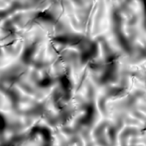
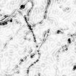
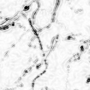
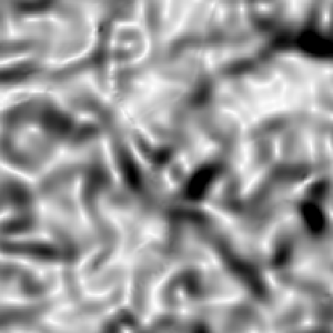
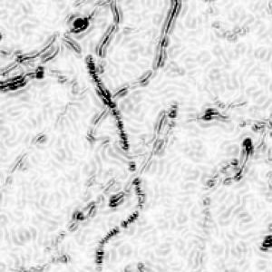
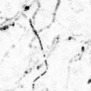
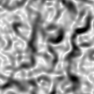
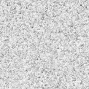
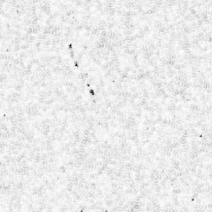
Figure 6: Magnitude of the gradient of the string signal before denoising (left panels), after Wiener filtering (middle panels) and WDBD (right panels), in the noise conditions PA$-$IN and for various string tensions at $1$ arcminute resolution on a field of view of $\tau^{\prime}=1.4^{\circ}$. From top to bottom, the string tensions considered are $\rho=2.5\times 10^{-7}$, $\rho=6.3\times 10^{-8}$, and $\rho=6.3\times 10^{-10}$.

\psfrag{2.2e-07}[0.9]{$2.2\times 10^{-7}$}\psfrag{2.5e-07}[0.9]{$2.5\times 10^{-7}$}\psfrag{2.8e-07}[0.9]{$2.8\times 10^{-7}$}\psfrag{5.6e-08}[0.9]{$5.6\times 10^{-8}$}\psfrag{6.3e-08}[0.9]{$6.3\times 10^{-8}$}\psfrag{7.0e-08}[0.9]{$7.0\times 10^{-8}$}\psfrag{5.6e-10}[0.9]{$5.6\times 10^{-10}$}\psfrag{6.3e-10}[0.9]{$6.3\times 10^{-10}$}\psfrag{7.0e-10}[0.9]{$7.0\times 10^{-10}$}\psfrag{0.05}[0.9]{0.05}\psfrag{0.04}[0.9]{0.04}\psfrag{0.03}[0.9]{0.03}\psfrag{0.02}[0.9]{0.02}\psfrag{0.01}[0.9]{0.01}\psfrag{0}[0.9]{0\hskip 20.00003pt}\includegraphics[width=142.26378pt]{figures/figure7_k1}

\psfrag{2.2e-07}[0.9]{$2.2\times 10^{-7}$}\psfrag{2.5e-07}[0.9]{$2.5\times 10^{-7}$}\psfrag{2.8e-07}[0.9]{$2.8\times 10^{-7}$}\psfrag{5.6e-08}[0.9]{$5.6\times 10^{-8}$}\psfrag{6.3e-08}[0.9]{$6.3\times 10^{-8}$}\psfrag{7.0e-08}[0.9]{$7.0\times 10^{-8}$}\psfrag{5.6e-10}[0.9]{$5.6\times 10^{-10}$}\psfrag{6.3e-10}[0.9]{$6.3\times 10^{-10}$}\psfrag{7.0e-10}[0.9]{$7.0\times 10^{-10}$}\psfrag{0.05}[0.9]{0.05}\psfrag{0.04}[0.9]{0.04}\psfrag{0.03}[0.9]{0.03}\psfrag{0.02}[0.9]{0.02}\psfrag{0.01}[0.9]{0.01}\psfrag{0}[0.9]{0\hskip 20.00003pt}\includegraphics[width=142.26378pt]{figures/figure7_k2}

\psfrag{2.2e-07}[0.9]{$2.2\times 10^{-7}$}\psfrag{2.5e-07}[0.9]{$2.5\times 10^{-7}$}\psfrag{2.8e-07}[0.9]{$2.8\times 10^{-7}$}\psfrag{5.6e-08}[0.9]{$5.6\times 10^{-8}$}\psfrag{6.3e-08}[0.9]{$6.3\times 10^{-8}$}\psfrag{7.0e-08}[0.9]{$7.0\times 10^{-8}$}\psfrag{5.6e-10}[0.9]{$5.6\times 10^{-10}$}\psfrag{6.3e-10}[0.9]{$6.3\times 10^{-10}$}\psfrag{7.0e-10}[0.9]{$7.0\times 10^{-10}$}\psfrag{0.05}[0.9]{0.05}\psfrag{0.04}[0.9]{0.04}\psfrag{0.03}[0.9]{0.03}\psfrag{0.02}[0.9]{0.02}\psfrag{0.01}[0.9]{0.01}\psfrag{0}[0.9]{0\hskip 20.00003pt}\includegraphics[width=142.26378pt]{figures/figure7_k3}

Figure 7: Posterior probability distributions (red solid curves) for the string tension as computed from simulated signals observed for $\rho=2.5\times 10^{-7}$ (left panel), $\rho=6.3\times 10^{-8}$ (middle panel), and $\rho=6.3\times 10^{-10}$ (right panel), in the noise conditions PA$-$IN at $1$ arcminute resolution. The black dashed vertical lines represent the exact values of the string tension relative to the test string simulation.

\psfrag{20}[0.9]{20}\psfrag{0}[0.9]{0\hskip 5.0pt}\psfrag{-20}[0.9]{-20}\psfrag{-40}[0.9]{-40}\psfrag{-60}[0.9]{-60}\psfrag{-80}[0.9]{}\psfrag{10}[0.9]{10}\psfrag{-10}[0.9]{-10}\psfrag{-9}[0.9]{-9}\psfrag{-8}[0.9]{-8}\psfrag{-7}[0.9]{-7}\psfrag{-6}[0.9]{-6}\psfrag{-5}[0.9]{-5}\psfrag{-0.5}[0.9]{-0.5}\psfrag{0.5}[0.9]{0.5}\psfrag{1}[0.9]{1}\psfrag{1.5}[0.9]{1.5}\psfrag{50}[0.9]{50}\psfrag{100}[0.9]{100}\psfrag{150}[0.9]{150}\psfrag{200}[0.9]{200}\psfrag{snrdb}{SNR (dB)}\psfrag{correlationcoefficient}{Correlation Coefficient}\psfrag{kurtosis}{Kurtosis}\psfrag{log10rho}{$\log_{10}(\rho)$}\includegraphics[width=142.26378pt]{figures/figure8_gradsnr}

\psfrag{20}[0.9]{20}\psfrag{0}[0.9]{0\hskip 5.0pt}\psfrag{-20}[0.9]{-20}\psfrag{-40}[0.9]{-40}\psfrag{-60}[0.9]{-60}\psfrag{-80}[0.9]{}\psfrag{10}[0.9]{10}\psfrag{-10}[0.9]{-10}\psfrag{-9}[0.9]{-9}\psfrag{-8}[0.9]{-8}\psfrag{-7}[0.9]{-7}\psfrag{-6}[0.9]{-6}\psfrag{-5}[0.9]{-5}\psfrag{-0.5}[0.9]{-0.5}\psfrag{0.5}[0.9]{0.5}\psfrag{1}[0.9]{1}\psfrag{1.5}[0.9]{1.5}\psfrag{50}[0.9]{50}\psfrag{100}[0.9]{100}\psfrag{150}[0.9]{150}\psfrag{200}[0.9]{200}\psfrag{snrdb}{SNR (dB)}\psfrag{correlationcoefficient}{Correlation Coefficient}\psfrag{kurtosis}{Kurtosis}\psfrag{log10rho}{$\log_{10}(\rho)$}\includegraphics[width=142.26378pt]{figures/figure8_gradcc}

\psfrag{20}[0.9]{20}\psfrag{0}[0.9]{0\hskip 5.0pt}\psfrag{-20}[0.9]{-20}\psfrag{-40}[0.9]{-40}\psfrag{-60}[0.9]{-60}\psfrag{-80}[0.9]{}\psfrag{10}[0.9]{10}\psfrag{-10}[0.9]{-10}\psfrag{-9}[0.9]{-9}\psfrag{-8}[0.9]{-8}\psfrag{-7}[0.9]{-7}\psfrag{-6}[0.9]{-6}\psfrag{-5}[0.9]{-5}\psfrag{-0.5}[0.9]{-0.5}\psfrag{0.5}[0.9]{0.5}\psfrag{1}[0.9]{1}\psfrag{1.5}[0.9]{1.5}\psfrag{50}[0.9]{50}\psfrag{100}[0.9]{100}\psfrag{150}[0.9]{150}\psfrag{200}[0.9]{200}\psfrag{snrdb}{SNR (dB)}\psfrag{correlationcoefficient}{Correlation Coefficient}\psfrag{kurtosis}{Kurtosis}\psfrag{log10rho}{$\log_{10}(\rho)$}\includegraphics[width=142.26378pt]{figures/figure8_kurt}

Figure 8: Signal-to-noise ratio (left panel) in decibels (dB), correlation coefficient (middle panel), and kurtosis (right panel) of the magnitude of gradient as functions of the string tension in logarithmic scaling in the range $\log_{10}\rho\in[-10,-05]$ in the noise conditions PA$-$IN and at $1$ arcminute resolution. The black dashed curves represent values before denoising, while the red solid curves and green dot-dashed curves represent values after WDBD and Wiener filtering respectively. The vertical lines on the curves represent the variability at one standard deviation of the estimated statistic across the $100$ test simulations considered (these lines are not visible where smaller than the width of the curves). The blue dotted vertical lines represent the eye visibility threshold $\rho=6.3\times 10^{-10}$. The blue dotted horizontal lines identify either the limit of zero signal-to-ratio, zero correlation coefficient, or the kurtosis of the magnitude of gradient of a pure string signal: $\kappa^{|\mathbf{\nabla}s|}\simeq 32$.

For the PA$-$IN condition, the magnitude of gradient of the string signal before and after WDBD and Wiener filtering is represented in Figure 6 for various string tensions from a single simulation. Only one fifth of the total field of view of the simulations is shown, corresponding to an angular opening $\tau^{\prime}=1.4^{\circ}$.

The visibility of the individual strings of the network is clearly enhanced by the denoising. For a value of the string tension around the experimental upper bound $\rho=2.5\times 10^{-7}$, part of the network is visible by eye before denoising. At tension $\rho=6.3\times 10^{-8}$, a very reduced number of strings is visible by eye before denoising. For both of these string tensions, part of the network is visible by eye through WDBD and Wiener filtering, but the resulting map is clearly more noisy in the second case. The value $\rho=6.3\times 10^{-10}$ is the lower bound on the string tension where a very reduced number of strings is visible by eye through WDBD, while no strings are visible by eye before denoising. In this limit, only string loops are actually recovered, together with some spurious point sources. Wiener filtering only provides noise at that level.

The posterior probability distributions for the string tension are reported in Figure 7 as computed from the signals observed at the three string tensions of interest in Figure 6. The graphs highlight the high precision of the localization of $\rho$ by the PSM described in Section 4. The slight offset observed is not related to a bias of the procedure itself but is simply due to an effective difference between the power spectrum of the test string simulation and the analytical expression of the power spectrum $P^{s}(k)$ used in relations (20) and (21). This difference may be associated with a cosmic variance including the contribution of a string signal.

The signal-to-noise ratio, correlation coefficient, and kurtosis of the magnitude of gradient of the string before and after WDBD and Wiener filtering are represented in Figure 8 as functions of the string tension. In the range of string tensions where the denoising procedure provides visibility of strings by eye, it appears clearly that WDBD and Wiener filtering both significantly increase the signal-to-noise ratio and correlation coefficient to strictly positive values. At low string tensions the correlation coefficient is also significantly higher for WDBD than for Wiener filtering. This represents a first quantitative measure of the superiority of our approach. The kurtosis of the magnitude of gradient is also significantly increased from its value before denoising towards higher values through WDBD. The peak obtained at low string tensions, with kurtosis values above the expected value around $\kappa^{|\mathbf{\nabla}s|}\simeq 32$, reflects the fact that the denoising recovers a thresholded version of the string signal in that range, only keeping localized loops in the limit identified by the visibility by eye (see Figure 6). At low string tensions, Wiener filtering essentially fails to increase the kurtosis values towards the expected value. We interpret this failure as a quantitative measure of the fact that Wiener filtering fails to remove a substantial part of the noise, in contrast with WDBD. This represents a second quantitative measure of the superiority of our approach. Let us emphasize that the lowest string tensions where each of our quantitative measures begin to show effective denoising performance for the WDBD algorithm are very close to the eye visibility threshold.

The degradation of the denoising performance due to instrumental noise is probed in the noise condition PA$+$IN, with an instrumental noise level of $1\mu K$. For this case we omit a complete analysis of all our quantitative measures. We simply notice that such a small level of instrumental noise already significantly affects the denoising performance by raising the eye visibility threshold by more than one order of magnitude. The only reason why an effective reconstruction of strings may be achieved down to so small string tensions in the noise conditions PA$-$IN is simply that, at high spatial frequencies, the string signal with a nearly scale-free power spectrum largely dominates the primary anisotropies with an exponentially damped power spectrum. This advantage is lost as soon as high frequency noise is added, in particular instrumental noise.

5.3 Noise conditions SA$-$tSZ and SA$+$tSZ

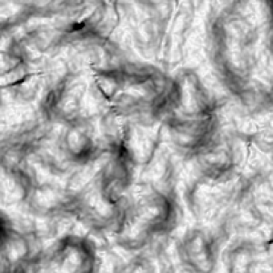
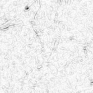
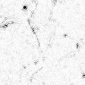
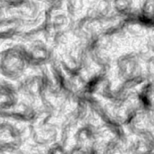
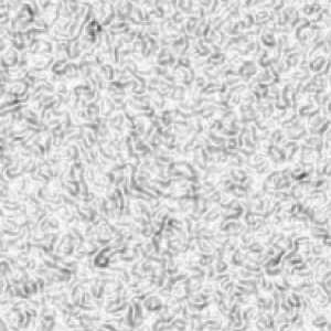
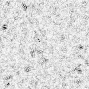
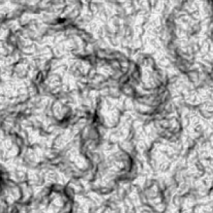
Figure 9: Magnitude of the gradient of the string signal before denoising (left panels), after Wiener filtering (middle panels) and WDBD (right panels), for various string tensions at $1$ arcminute resolution on a field of view of $\tau^{\prime}=1.4^{\circ}$. The two top panel rows relate to the noise conditions SA$-$tSZ for string tensions $\rho=4.0\times 10^{-7}$ and $\rho=1.0\times 10^{-7}$ respectively. The bottom panel row relates to the noise conditions SA$+$tSZ for a string tension $\rho=2.5\times 10^{-7}$.

\psfrag{3.6e-07}[0.9]{$3.6\times 10^{-7}$}\psfrag{4.0e-07}[0.9]{$4.0\times 10^{-7}$}\psfrag{4.4e-07}[0.9]{$4.4\times 10^{-7}$}\psfrag{8.9e-08}[0.9]{$8.9\times 10^{-8}$}\psfrag{1.0e-07}[0.9]{$1.0\times 10^{-7}$}\psfrag{1.1e-07}[0.9]{$1.1\times 10^{-7}$}\psfrag{2.2e-07}[0.9]{$2.2\times 10^{-7}$}\psfrag{2.5e-07}[0.9]{$2.5\times 10^{-7}$}\psfrag{2.8e-07}[0.9]{$2.8\times 10^{-7}$}\psfrag{0.05}[0.9]{0.05}\psfrag{0.04}[0.9]{0.04}\psfrag{0.03}[0.9]{0.03}\psfrag{0.025}[0.9]{0.025}\psfrag{0.02}[0.9]{0.02}\psfrag{0.015}[0.9]{0.015}\psfrag{0.01}[0.9]{0.01}\psfrag{0.005}[0.9]{0.005}\psfrag{0}[0.9]{0\hskip 20.00003pt}\includegraphics[width=142.26378pt]{figures/figure10_k1}

\psfrag{3.6e-07}[0.9]{$3.6\times 10^{-7}$}\psfrag{4.0e-07}[0.9]{$4.0\times 10^{-7}$}\psfrag{4.4e-07}[0.9]{$4.4\times 10^{-7}$}\psfrag{8.9e-08}[0.9]{$8.9\times 10^{-8}$}\psfrag{1.0e-07}[0.9]{$1.0\times 10^{-7}$}\psfrag{1.1e-07}[0.9]{$1.1\times 10^{-7}$}\psfrag{2.2e-07}[0.9]{$2.2\times 10^{-7}$}\psfrag{2.5e-07}[0.9]{$2.5\times 10^{-7}$}\psfrag{2.8e-07}[0.9]{$2.8\times 10^{-7}$}\psfrag{0.05}[0.9]{0.05}\psfrag{0.04}[0.9]{0.04}\psfrag{0.03}[0.9]{0.03}\psfrag{0.025}[0.9]{0.025}\psfrag{0.02}[0.9]{0.02}\psfrag{0.015}[0.9]{0.015}\psfrag{0.01}[0.9]{0.01}\psfrag{0.005}[0.9]{0.005}\psfrag{0}[0.9]{0\hskip 20.00003pt}\includegraphics[width=142.26378pt]{figures/figure10_k2}

\psfrag{3.6e-07}[0.9]{$3.6\times 10^{-7}$}\psfrag{4.0e-07}[0.9]{$4.0\times 10^{-7}$}\psfrag{4.4e-07}[0.9]{$4.4\times 10^{-7}$}\psfrag{8.9e-08}[0.9]{$8.9\times 10^{-8}$}\psfrag{1.0e-07}[0.9]{$1.0\times 10^{-7}$}\psfrag{1.1e-07}[0.9]{$1.1\times 10^{-7}$}\psfrag{2.2e-07}[0.9]{$2.2\times 10^{-7}$}\psfrag{2.5e-07}[0.9]{$2.5\times 10^{-7}$}\psfrag{2.8e-07}[0.9]{$2.8\times 10^{-7}$}\psfrag{0.05}[0.9]{0.05}\psfrag{0.04}[0.9]{0.04}\psfrag{0.03}[0.9]{0.03}\psfrag{0.025}[0.9]{0.025}\psfrag{0.02}[0.9]{0.02}\psfrag{0.015}[0.9]{0.015}\psfrag{0.01}[0.9]{0.01}\psfrag{0.005}[0.9]{0.005}\psfrag{0}[0.9]{0\hskip 20.00003pt}\includegraphics[width=142.26378pt]{figures/figure10_k3}

Figure 10: Posterior probability distributions (red solid curves) for the string tension as computed from a simulated signal observed at $1$ arcminute resolution. The left and middle panels relate to the noise conditions SA$-$tSZ for string tensions $\rho=4.0\times 10^{-7}$ and $\rho=1.0\times 10^{-7}$ respectively. The right panel relates to the noise conditions SA$+$tSZ for a string tension $\rho=2.5\times 10^{-7}$. The black dashed vertical lines represent the exact values of the string tension relative to the test string simulation.

\psfrag{20}[0.9]{20}\psfrag{0}[0.9]{0\hskip 5.0pt}\psfrag{-20}[0.9]{-20}\psfrag{-40}[0.9]{-40}\psfrag{-60}[0.9]{-60}\psfrag{-80}[0.9]{}\psfrag{10}[0.9]{10}\psfrag{-10}[0.9]{-10}\psfrag{-9}[0.9]{-9}\psfrag{-8}[0.9]{-8}\psfrag{-7}[0.9]{-7}\psfrag{-6}[0.9]{-6}\psfrag{-5}[0.9]{-5}\psfrag{-0.5}[0.9]{-0.5}\psfrag{0.5}[0.9]{0.5}\psfrag{1}[0.9]{1}\psfrag{1.5}[0.9]{1.5}\psfrag{50}[0.9]{50}\psfrag{100}[0.9]{100}\psfrag{150}[0.9]{150}\psfrag{200}[0.9]{200}\psfrag{snrdb}{SNR (dB)}\psfrag{correlationcoefficient}{Correlation Coefficient}\psfrag{kurtosis}{Kurtosis}\psfrag{log10rho}{$\log_{10}(\rho)$}\includegraphics[width=142.26378pt]{figures/figure11_gradsnr_secminf}

\psfrag{20}[0.9]{20}\psfrag{0}[0.9]{0\hskip 5.0pt}\psfrag{-20}[0.9]{-20}\psfrag{-40}[0.9]{-40}\psfrag{-60}[0.9]{-60}\psfrag{-80}[0.9]{}\psfrag{10}[0.9]{10}\psfrag{-10}[0.9]{-10}\psfrag{-9}[0.9]{-9}\psfrag{-8}[0.9]{-8}\psfrag{-7}[0.9]{-7}\psfrag{-6}[0.9]{-6}\psfrag{-5}[0.9]{-5}\psfrag{-0.5}[0.9]{-0.5}\psfrag{0.5}[0.9]{0.5}\psfrag{1}[0.9]{1}\psfrag{1.5}[0.9]{1.5}\psfrag{50}[0.9]{50}\psfrag{100}[0.9]{100}\psfrag{150}[0.9]{150}\psfrag{200}[0.9]{200}\psfrag{snrdb}{SNR (dB)}\psfrag{correlationcoefficient}{Correlation Coefficient}\psfrag{kurtosis}{Kurtosis}\psfrag{log10rho}{$\log_{10}(\rho)$}\includegraphics[width=142.26378pt]{figures/figure11_gradcc_secminf}

\psfrag{20}[0.9]{20}\psfrag{0}[0.9]{0\hskip 5.0pt}\psfrag{-20}[0.9]{-20}\psfrag{-40}[0.9]{-40}\psfrag{-60}[0.9]{-60}\psfrag{-80}[0.9]{}\psfrag{10}[0.9]{10}\psfrag{-10}[0.9]{-10}\psfrag{-9}[0.9]{-9}\psfrag{-8}[0.9]{-8}\psfrag{-7}[0.9]{-7}\psfrag{-6}[0.9]{-6}\psfrag{-5}[0.9]{-5}\psfrag{-0.5}[0.9]{-0.5}\psfrag{0.5}[0.9]{0.5}\psfrag{1}[0.9]{1}\psfrag{1.5}[0.9]{1.5}\psfrag{50}[0.9]{50}\psfrag{100}[0.9]{100}\psfrag{150}[0.9]{150}\psfrag{200}[0.9]{200}\psfrag{snrdb}{SNR (dB)}\psfrag{correlationcoefficient}{Correlation Coefficient}\psfrag{kurtosis}{Kurtosis}\psfrag{log10rho}{$\log_{10}(\rho)$}\includegraphics[width=142.26378pt]{figures/figure11_kurt_secminf}

\psfrag{20}[0.9]{20}\psfrag{0}[0.9]{0\hskip 5.0pt}\psfrag{-20}[0.9]{-20}\psfrag{-40}[0.9]{-40}\psfrag{-60}[0.9]{-60}\psfrag{-80}[0.9]{}\psfrag{10}[0.9]{10}\psfrag{-10}[0.9]{-10}\psfrag{-9}[0.9]{-9}\psfrag{-8}[0.9]{-8}\psfrag{-7}[0.9]{-7}\psfrag{-6}[0.9]{-6}\psfrag{-5}[0.9]{-5}\psfrag{-0.5}[0.9]{-0.5}\psfrag{0.5}[0.9]{0.5}\psfrag{1}[0.9]{1}\psfrag{1.5}[0.9]{1.5}\psfrag{50}[0.9]{50}\psfrag{100}[0.9]{100}\psfrag{150}[0.9]{150}\psfrag{200}[0.9]{200}\psfrag{snrdb}{SNR (dB)}\psfrag{correlationcoefficient}{Correlation Coefficient}\psfrag{kurtosis}{Kurtosis}\psfrag{log10rho}{$\log_{10}(\rho)$}\includegraphics[width=142.26378pt]{figures/figure11_gradsnr_sec0}

\psfrag{20}[0.9]{20}\psfrag{0}[0.9]{0\hskip 5.0pt}\psfrag{-20}[0.9]{-20}\psfrag{-40}[0.9]{-40}\psfrag{-60}[0.9]{-60}\psfrag{-80}[0.9]{}\psfrag{10}[0.9]{10}\psfrag{-10}[0.9]{-10}\psfrag{-9}[0.9]{-9}\psfrag{-8}[0.9]{-8}\psfrag{-7}[0.9]{-7}\psfrag{-6}[0.9]{-6}\psfrag{-5}[0.9]{-5}\psfrag{-0.5}[0.9]{-0.5}\psfrag{0.5}[0.9]{0.5}\psfrag{1}[0.9]{1}\psfrag{1.5}[0.9]{1.5}\psfrag{50}[0.9]{50}\psfrag{100}[0.9]{100}\psfrag{150}[0.9]{150}\psfrag{200}[0.9]{200}\psfrag{snrdb}{SNR (dB)}\psfrag{correlationcoefficient}{Correlation Coefficient}\psfrag{kurtosis}{Kurtosis}\psfrag{log10rho}{$\log_{10}(\rho)$}\includegraphics[width=142.26378pt]{figures/figure11_gradcc_sec0}

\psfrag{20}[0.9]{20}\psfrag{0}[0.9]{0\hskip 5.0pt}\psfrag{-20}[0.9]{-20}\psfrag{-40}[0.9]{-40}\psfrag{-60}[0.9]{-60}\psfrag{-80}[0.9]{}\psfrag{10}[0.9]{10}\psfrag{-10}[0.9]{-10}\psfrag{-9}[0.9]{-9}\psfrag{-8}[0.9]{-8}\psfrag{-7}[0.9]{-7}\psfrag{-6}[0.9]{-6}\psfrag{-5}[0.9]{-5}\psfrag{-0.5}[0.9]{-0.5}\psfrag{0.5}[0.9]{0.5}\psfrag{1}[0.9]{1}\psfrag{1.5}[0.9]{1.5}\psfrag{50}[0.9]{50}\psfrag{100}[0.9]{100}\psfrag{150}[0.9]{150}\psfrag{200}[0.9]{200}\psfrag{snrdb}{SNR (dB)}\psfrag{correlationcoefficient}{Correlation Coefficient}\psfrag{kurtosis}{Kurtosis}\psfrag{log10rho}{$\log_{10}(\rho)$}\includegraphics[width=142.26378pt]{figures/figure11_kurt_sec0}

Figure 11: Signal-to-noise ratio (left panels) in decibels (dB), correlation coefficient (middle panels), and kurtosis (right panels) of the magnitude of gradient as functions of the string tension in logarithmic scaling in the range $\log_{10}\rho\in[-10,-05]$ and at $1$ arcminute resolution. The top panels relate to the noise conditions SA$-$tSZ, while the bottom panels relate to the noise conditions SA$+$tSZ. The black dashed curves represent values before denoising, while the red solid curves and green dot-dashed curves represent values after WDBD and Wiener filtering respectively. The vertical lines on the curves represent the variability at one standard deviation of the estimated statistic across the $100$ test simulations considered (these lines are not visible by eye where smaller than the width of the curves). The blue dotted vertical lines represent the eye visibility thresholds $\rho=1.0\times 10^{-7}$ for the top panels and $\rho=2.5\times 10^{-7}$ for the bottom panels. The blue dotted horizontal lines identify either the limit of zero signal-to-ratio, zero correlation coefficient, or the kurtosis of the magnitude of gradient of a pure string signal: $\kappa^{|\mathbf{\nabla}s|}\simeq 32$.

The magnitude of gradient of the string signal before and after WDBD and Wiener filtering is represented in Figure 9 for various string tensions, from a single simulation. In the noise conditions SA$-$tSZ and for a value of the string tension around the experimental upper bound $\rho=4.0\times 10^{-7}$, a very reduced number of strings is visible by eye before denoising. Part of the network is visible by eye after WDBD and Wiener filtering, but the resulting map is clearly more noisy in the second case. The value $\rho=1.0\times 10^{-7}$ is the lower bound on the string tension where a very reduced number of strings is visible by eye through WDBD, while no string is visible by eye before denoising. Wiener filtering only provides noise at that level. In the noise conditions SA$+$tSZ, the value $\rho=2.5\times 10^{-7}$ is the lower bound on the string tension where a very reduced number of strings is visible by eye through WDBD, while no string is visible by eye before denoising. Again, Wiener filtering only provides noise at that level. At the lower bounds for the string tensions in both noise conditions only string loops are recovered, still with some spurious point sources.

The posterior probability distributions for the string tension are reported in Figure 10 as computed from the signals observed in the three cases of interest in Figure 9. The graphs still highlight the high precision of the localization of $\rho$ by the PSM.

The signal-to-noise ratio, correlation coefficient, and kurtosis of the magnitude of gradient of the string signal before and after WDBD and Wiener filtering are represented in Figure 11 as functions of the string tension. As for the PA$-$IN and PA$+$IN cases, both WDBD and Wiener filtering increase the signal-to-noise ratio and correlation coefficient to strictly positive values for tensions above the eye visibility threshold. The correlation coefficient is significantly higher for WDBD than for Wiener filtering in the whole range of string tensions of interest. As before, the kurtosis of the magnitude of gradient is also significantly increased from its value before denoising towards higher values through WDBD, with a peak at low string tensions due to the fact that the denoising recovers a thresholded version of the string signal. Wiener filtering essentially fails to increase the kurtosis values towards the expected value in the whole range of string tensions of interest, once more reflecting its poorer denoising performance. As before, we see that for both SA$-$tSZ and SA$+$tSZ, the eye visibility thresholds are very close to the lowest string tensions where each of our quantitative measures begin to show effective denoising performance.

Let us acknowledge the fact that, in the noise conditions SA$-$tSZ and SA$+$tSZ, the lowest string tensions where denoising is effective are greatly increased relative to the noise condition PA$-$IN. For SA$-$tSZ, the eye visibility threshold is slightly below the best experimental bound, while for SA$+$tSZ it is slightly above. These results are absolutely in the line of those obtained in the noise condition PA$+$IN, as the secondary anisotropies represent even stronger higher frequency noise.

5.4 Comparison to PSM detectability threshold

Noise condition	PSM detectability	Eye visibility
PA$-$IN	$2.2\times 10^{-10}$	$6.3\times 10^{-10}$
PA$+$IN	$1.7\times 10^{-8}$	$2.5\times 10^{-8}$
SA$-$tSZ	$6.1\times 10^{-8}$	$1.0\times 10^{-7}$
SA$+$tSZ	$1.9\times 10^{-7}$	$2.5\times 10^{-7}$

Table 2: PSM detectability and eye visibility thresholds on the string tension determined on the basis of the PSM for each of the noise conditions considered. All values are given with two significant figures.

As our WDBD algorithm uses the PSM for preliminary localization of the string tension, it is a natural question to ask whether the overall denoising performance at low string tensions is limited by this preliminary PSM localization. We address this by defining and studying the detectability threshold for the PSM, which provides a measure of the minimum string tension where the PSM alone provides robust detection of strings.

We firstly describe how the PSM detection threshold is computed, based on a hypothesis test for string detection. We may define an estimation $\widehat{\rho}$ of the string tension from the observed signal $f$ as the expectation value of the posterior probability distribution (21) computed on the basis of the PSM:

$$\widehat{\rho}=E\left[p\left(\rho|\widehat{f}\right)\right].$$ (28)

For any possible string tension, the probability distribution function for $\widehat{\rho}$ may consequently be obtained from simulations.

We identify the critical value $\rho_{0}$ such that, for null string tension, one has $p(\widehat{\rho}\geq\rho_{0})=\alpha$, for some suitable positive value $\alpha$ much smaller than unity. The test for the hypothesis of null string tension is then defined as follows. For estimated values $\widehat{\rho}\geq\rho_{0}$, the hypothesis of null string tension may be rejected with a significance level $\alpha$. On the contrary for estimated values $\widehat{\rho}<\rho_{0}$, the hypothesis of null string tension may not be rejected.

We define the detectability threshold $\rho^{\star}$ such that, for a string tension $\rho^{\star}$, one has $p(\widehat{\rho}\geq\rho_{0})=1-\beta$, for some other suitable positive value $\beta$ much smaller than unity. Consequently, for string tensions larger than $\rho^{\star}$, the probability of rejecting a null string tension on the basis of the hypothesis test defined is larger than $1-\beta$. The value $\rho^{\star}$ is the smallest string tension that can be discriminated from the hypothesis of null string tension for given values of $\alpha$ and $\beta$. It may thus be understood as a detectability threshold determined on the basis of the PSM. As our overall denoising method is using the PSM as a preliminary estimation of the string tension, $\rho^{\star}$ identifies an effective lower bound on the string tension range where denoising could reasonably be expected to be effective.

The PSM detectability thresholds in the various noise conditions considered are reported in Table 2 for $\alpha\simeq\beta\simeq 0.01$. In all cases except SA$+$tSZ the PSM detectability thresholds are below the best experimental bound, while for SA$+$tSZ the PSM detectability threshold is around the best experimental bound.

Secondly, we compare these thresholds with the eye visibility thresholds, which as noted previously also indicate the lower limit of string tensions where our quantitative measures show effective performance for the WDBD algorithm. For each of the noise conditions with significant high frequency content, i.e. PA$+$IN, SA$-$tSZ and SA$+$tSZ, the PSM detectability threshold $\rho^{*}$ is slightly below the eye visibility threshold. For the PA$-$IN case, this difference is larger, the PSM detectability threshold being about one third of the eye visibility threshold. This indicates that the PSM is able to more effectively exploit the high spatial frequency ranges where the string signal dominates the primary anisotropies.

The discrepancy between these two thresholds shows that the detection problem alone can be solved with the PSM at slightly lower string tensions than the more difficult denoising problem. Indeed for values of the string tension between the two thresholds, denoising does not produce visible strings even though the PSM posterior probability distributions for $\rho$ are distinctly peaked away from zero. It is one thing to estimate a single global parameter such as the string tension on the basis of a PSM, but quite another to explicitly reconstruct the string network itself.

5.5 Algorithm robustness

We comment here on the robustness of the WDBD algorithm relative to both additional noise from foreground point sources and to the possible improvements in the definition of the denoising procedure itself.

We have explicitly disregarded the problem of foreground emissions such as radio and infrared point sources. The discrimination of point sources from string loops imprinted in the CMB may appear to be a difficult task. However, the dipolar structure of the string loops represents an essential difference with point sources (Fraisse et al., 2008). In that context, the odd symmetry of the wavelets used in the WDBD algorithm (see Figure 3) to match the string imprints is adequate both for long strings and string loops, and might help to discriminate between string loops and point sources. The algorithm was shown to be effective at detecting string loops, even at low tensions where long strings are not reconstructed anymore. However spurious point sources were also reconstructed at very small string tensions in the noise conditions PA$-$IN, in the absence of foreground point sources. A thorough analysis should be conducted in order to assess the real robustness of the algorithm to discriminate between string loops and point sources, and to discuss necessary enhancements.

Our approach explicitly assumes the statistical independence of coefficients of the wavelet decomposition, when conditioned on the string tension. However, significant correlations are present in the wavelet coefficients, and exploiting them should lead to improved denoising performance. Gaussian scale mixture (GSM) models may be considered which allow one to explicitly account for local correlations of the wavelet coefficients in the denoising process (Andrews & Mallows, 1974; Portilla et al., 2003). An enhanced version of this model called the orientation-adapted Gaussian scale mixture (OAGSM) model relies on steerable wavelets in order to integrate directionality information in the local correlations (Hammond & Simoncelli, 2008). A preliminary implementation of the OAGSM model suggests that an enhancement relative to the WDBD algorithm may indeed be expected, albeit at significant computational cost.

An improvement of the similarity of the shape of the filters to better match the typical string imprints may also be envisaged. Even though steerable wavelets can be very directional, their spatial support is not especially narrow. Filters with a more elongated support such as curvelets (Candès & Donoho, 1999; Starck et al., 2002) might be expected to provide better performance for the detection of long strings. Let us notice however that such filters would not be adequate anymore for string loops. Moreover a preliminary implementation of this evolution provides no improvement relative to the WDBD algorithm for the detection of long strings.

Finally, a discretization of the wavelet scales finer than the dyadic discretization used might provide an improved statistical model of the coefficients of the string signal at each spatial scale $b$. We did not consider this evolution here.

6 Conclusion

We have described a Bayesian framework for mapping the CMB signal induced by cosmic strings, based on a generalized Gaussian model capturing the sparse behaviour of the string signal in the steerable wavelet domain. This signal is buried in the standard primary and secondary CMB anisotropies, which we model as Gaussian noise. For a fixed string tension we compute the Bayesian least squares estimator for each wavelet coefficient of the string signal. Our overall estimator is then formed as an average of these estimates for different string tensions, weighted by the posterior probability of the string tension under a power spectral model.

We have demonstrated the performance of our denoising algorithm through a series of numerical analyses at $1$ arcminute resolution consistent with upcoming experiments. The maps of the magnitude of the gradient of the denoised string signal produced by our algorithm were evaluated on the basis of three quantitative measures: the signal-to-noise ratio and correlation coefficient computed with respect to the known original string signal, and the kurtosis. In the idealized case of primary anisotropies without instrumental noise, the strings can be identified for tensions down to $\rho=6.3\times 10^{-10}$, more than two orders of magnitude below the current experimental upper bound. With instrumental noise around $1\,\mu\textnormal{K}$ per pixel this lower bound is increased by more than one order of magnitude. The inclusion of secondary anisotropies further raises this bound to $\rho=1.0\times 10^{-7}$ disregarding the thermal Sunyaev-Zel’dovich effect and to $\rho=2.5\times 10^{-7}$ including this effect in the Rayleigh-Jeans limit. These values nonetheless remain slightly below or near the current experimental upper bound on the string tension, demonstrating that the proposed algorithm will be useful for analysis of upcoming high resolution data.

References

- Albrecht & Turok (1985) Albrecht A., Turok N., 1985, Phys. Rev. Lett., 54, 1868
- Albrecht & Turok (1989) Albrecht A., Turok N., 1989, Phys. Rev. Lett., 40, 973
- Allen & Shellard (1990) Allen B., Shellard E. P. S., 1990, Phys. Rev. Lett., 64, 119
- Amsel et al. (2007) Amsel S., Berger J., Brandenberger R. H., 2008, JCAP, 04, 015
- Andrews & Mallows (1974) Andrews D., Mallows C., 1974, J. Royal Stat. Soc. B, 36, 99
- Antonini et al. (1992) Antonini M., Barlaud M., Mathieu P., Daubechies I., 1992, IEEE Trans. Image Proc., 1, 205
- Barker et al. (2006) Barker R. et al., 2006, MNRAS, 369, L1
- Barreiro & Hobson (2001) Barreiro R. B., Hobson M. P., 2001, 327, 813
- Belge et al. (2000) Belge M., Kilmer M. E., Miller E. L., 2000, IEEE Trans. Image Proc., 9, 597
- Bennet (1986) Bennet D. P., 1986, Phys. Rev. D, 33, 872
- Bennet & Bouchet (1989) Bennet D. P., Bouchet F. R., 1989, Phys. Rev. Lett., 63, 2776
- Bennet & Bouchet (1990) Bennet D. P., Bouchet F. R., 1990, Phys. Rev. D, 41, 2408
- Bennett et al. (2003) Bennett C.L. et al., 2003, ApJS, 148, 1
- Bevis et al. (2004) Bevis N., Hindmarsh M., Kunz M., 2004, Phys. Rev. D, 70, 043508
- Bevis et al. (2007) Bevis N., Hindmarsh M., Kunz M., Urrestilla J., 2007, Phys. Rev. D, 75, 065015
- Bobin et al. (2008) Bobin J., Moudden Y., Starck J.-L., Fadili J., Aghanim N., 2008, Stat. Method., 5, 307
- Bouchet et al. (1988) Bouchet F. R., Bennet D. P., Stebbins A., 1988, Nature, 335, 410
- Bouchet (2004) Bouchet F. R., 2004, preprint (arXiv:astro-ph/0401108v1)
- Candès & Donoho (1999) Candès E., Donoho D. L., 1999, in Cohen A., Rabut C., Schumaker L. L., eds, Curve and Surface fitting: Saint-Malo 1999. Vanderbilt University Press, Nashville, p. 105
- Davis & Kibble (2005) Davis A. C., Kibble T. W. B., 2005, Contemp. Phys., 46, 313
- Delabrouille et al. (2003) Delabrouille J., Cardoso J.-F., Patanchon G., 2003, MNRAS, 346, 1089
- Forni & Aghanim (2004) Forni O., Aghanim N., 2004, A&A, 420, 49
- Fraisse et al. (2007) Fraisse A. A., 2007, JCAP, 03, 008
- Fraisse et al. (2008) Fraisse A. A., Ringeval C., Spergel D. N., Bouchet F. R., 2008, Phys. Rev. D, 78, 043535
- Gott (1985) Gott J. R., 1985. ApJ, 288, 422
- Gull & Skilling (1999) Gull S. F., Skilling J., 1999. Quantified Maximum Entropy, MemSys5 Users’ Manual. Maximum Entropy Data Consultants Ltd., Suffolk
- Hammond & Simoncelli (2008) Hammond D. K., Simoncelli E. P., 2008, IEEE Trans. Image Proc., 17, 2089
- Hindmarsh (1995a) Hindmarsh M., 1995, Nucl. Phys. Proc. Suppl., 43, 50
- Hindmarsh & Kibble (1995b) Hindmarsh M., Kibble T. W. B., 1995, Rep. Prog. Phys., 58, 477
- Hinshaw et al. (2007) Hinshaw G. et al., 2007, ApJS, 170, 288
- Hinshaw et al. (2009) Hinshaw G. et al., 2009, ApJS, 180, 225
- Hobson et al. (1998) Hobson M. P., Jones A. W., Lasenby A. N., Bouchet F. R., 1998, MNRAS, 300, 1
- Hobson et al. (1999) Hobson M. P., Jones A. W., Lasenby A. N., 1999, MNRAS, 309, L125
- Jeong & Smoot (2005) Jeong E., Smoot G. F., 2005, ApJ, 624, 21
- Jones et al. (2002) Jones M. E., 2002, in Chen L.-W., Ma C.-P., Ng K.-W., Pen U.-L., eds, ASP Conf. Ser. Vol. 257, AMiBA 2001: High-z Clusters, Missing Baryons, and CMB Polarization. Astron. Soc. Pac., San Francisco, p. 35
- Jones et al. (2006) Jones W. C. et al., 2006, ApJ, 647, 823
- Kaiser & Stebbins (1984) Kaiser N., Stebbins A., 1984, Nature, 310, 391
- Kibble (1985) Kibble T. W. B., 1985, Nucl. Phys. B, 252, 227
- Komatsu & Seljak (2002) Komatsu E., Seljak U., 2002, MNRAS, 336, 1256
- Komatsu et al. (2009) Komatsu E. et al., 2009, ApJS, 180, 330
- Kosowsky (2006) Kosowsky A., 2006, New Astron. Rev., 50, 969
- Lo & Wright (2005) Lo A. S., Wright E. L., 2005, Bull. of the AAS, 37, 1429
- Maisinger et al. (1999) Maisinger K., Hobson M. P., Lasenby A. N., 2004, MNRAS, 347, 339
- Mallat (1998) Mallat S. G., 1998, A wavelet tour of signal processing. Academic Press, San Diego
- Moulin & Liu (1999) Moulin P., Liu J.,1999, IEEE Trans. Information Theo., 45, 909
- Moessner et al. (1994) Moessner R., Perivolaropoulos L., Brandenberger R., 1994, ApJ, 425, 365
- Perivolaropoulos (1993) Perivolaropoulos L., 1993, Phys. Lett. B, 1993, 305
- Pires et al. (2006) Pires S., Juin J.-B., Yvon D., Moudden Y., Anthoine S., Pierpaoli E., 2006, A&A, 455, 741
- Portilla et al. (2003) Portilla J., Strela V., Wainwright M. J., Simoncelli E. P., 2003, IEEE Trans. Image Proc., 12, 1338
- Readhead et al. (2004) Readhead A. C. S. et al., 2004, ApJ, 609, 498
- Reichardt et al. (2009) Reichardt et al., 2009, ApJ, 694, 1200
- Rocha et al. (2005) Rocha G., Hobson M. P., Smith S., Ferreira P., Challinor A., 2005, MNRAS, 357, 1
- Ruhl et al. (2004) Ruhl J. E. et al., 2004, in Zmuidzinas J., Holland W. S., and Withington S., eds, Proc. SPIE Conf. Vol. 5498, Millimeter and Submillimeter Detectors for Astronomy II. SPIE, Bellingham, p. 11
- Simoncelli et al. (1992) Simoncelli E. P., Freeman W. T., Adelson E. H., Heeger D. J., 1992, IEEE Trans. Information Theo., 38, 587
- Simoncelli & Adelson (1996) Simoncelli E. P., Adelson E. H., 1996, Proc. IEEE Conf. Vol. I. IEEE Signal Proc. Soc., p. 379
- Spergel et al. (2003) Spergel D. N. et al., 2003, ApJS, 148, 175
- Spergel et al. (2007) Spergel D. N. et al., 2007, ApJS, 170, 377
- Starck et al. (2002) Starck J.-L., Candès E., Donoho D. L., 2002, IEEE Trans. Image Proc., 11, 670
- Starck et al. (2006a) Starck J.-L., Murtagh F., 2006a, Astronomical Image and Data Analysis (Second Edition). Springer, Berlin
- Sunyaev & Zel’dovich (1980) Sunyaev R. A., Zel’dovich Y. B., 1980, Ann. Rev. Astron. Astrophys, 18, 537
- Turok & Spergel (1990) Turok N., Spergel D. N., 1990, Phys. Rev. Lett. 64, 2736
- Vachaspati & Vilenkin (1984) Vachaspati T., Vilenkin A., 1984, Phys. Rev. D, 30, 2036
- Vilenkin & Shellard (1994) Vilenkin A., Shellard E. P. S., 1994, Cosmic Strings and Other Topological Defects. Cambridge Univ. Press, Cambridge
- Wyman et al. (2005) Wyman M., Pogosian L., Wasserman I., 2005, Phys. Rev. D, 72, 023513
- Wyman et al. (2006) Wyman M., Pogosian L., Wasserman I., 2006, Phys. Rev. D, 73, 089905(E)
- Zwart et al. (2008) Zwart J. T. L., 2008, 391, 1545