Tunneling Time in the Landau-Zener Model

Abstract

We give a general definition for the tunneling time in the Landau-Zener model. This definition allows us to compute numerically the Landau-Zener tunneling time at any sweeping rate without ambiguity. We have also obtained analytical results in both the adiabatic limit and the sudden limit. Whenever applicable, our results are compared to previous results and they are in good agreement.

I INTRODUCTION

Tunneling is one of many fundamental quantum processes that have no classical counterparts. It exists ubiquitously in quantum systems and is a key to understanding many quantum phenomenaLZ7 ; LZ302 ; LZ301 ; LZ30 ; LL1 ; LL2 ; LL3 ; LZ33 ; LZ32 ; LZy ; LZy1 ; app . Discussions on tunneling can be found in all textbooks on quantum mechanics. However, these discussions are mainly focused on the probability of tunneling from one quantum state to another or from one side of a potential barrier to the other. In contrast, there are only a few extensive and in-depth discussions in literature on another aspect of tunneling, the time of tunneling, that is, how long a tunneling process lastsPZ1 ; PZ2 ; PZ3 ; PZ4 ; PZ5 ; LZ3 . This disparity is partly caused by the difficulty to define properly tunneling times in many situations.

The difficulty of having a proper definition for tunneling time has its root in the wave or probabilistic nature of quantum mechanics, and is best demonstrated in the example of a wave packet tunneling through a potential barrier. In this case, one would intuitively define the tunneling time as the time spent by the peak (or centroid) of the wave packet under the barrier. However, as pointed out by Landauer and MartinPZ51 , if this definition was used, a packet could leave the barrier before entering it. To overcome this difficulty, many different definitions have been suggested, and no clear consensus has been reached so farPZ0 .

The focus of this study is on the tunneling time in the Landau-Zener (LZ) modelLZ1 ; LZ2 . This system is much simpler than the wave packet and barrier system. Nevertheless, a proper definition of tunneling time in this model is still missing in spite of the studies in the past by many authors. Mullen et al. LZ8 discussed the LZ tunneling time in the diabatic basis for the two limiting cases, the adabatic limit and the sudden limit. They found that for large $\Delta$ (the adiabatic limit), the tunneling time scales with $\Delta/\alpha$ and for small $\Delta$ (the sudden limit), the tunneling time is about $\sqrt{\hbar/\alpha}$. $\Delta$ is the minimal energy gap between the two eigenstates in the LZ model and $\alpha$ is the sweeping rate. However, Mullen et al. did not give a general definition for the tunneling time. VitanovLZ5 has given a much more thorough study on the LZ tunneling time. He obtained analytical results for the LZ tunneling time in both diabatic and adiabatic bases. Furthermore, Vitanov tried to give a general definition for the tunneling time. However, his definition fails in certain cases, in particular, the adiabatic limit.

In this paper, we give a general definition for the tunneling time in the LZ model. We show both analytically and numerically that this definition yields reasonable results at any sweeping rate in both adiabatic basis and diabatic basis. With this general definition, we are able to reproduce the previous results obtained by Mullen et al.LZ8 and VitanovLZ5 . Furthermore, we are able to compute analytically the tunneling time in the adiabatic basis at the adiabatic limit, which is given by $2\sqrt{2^{1/3}-1}\Delta/\alpha$. This, to our best knowledge, has not been obtained before.

Besides it theoretical significance, our work has also potential applications. In the Monte-Carlo simulation of quantum tunneling in molecular magnets, the authors in Ref.LZ4 have used an empirical formula for the LZ tunneling time. This formula, given by $\sqrt{\Delta^{2}/\alpha^{2}+2\hbar/\alpha}$ and interpolating the two limiting results in Ref.LZ8 , is not well founded. With this newly-proposed definition, one no longer needs this empirical formula to do the Monte-Carlo simulation.

We note here that it is important to study the tunneling time in both the diabatic basis and the adiabatic basis. When the LZ model is applied to the case of the tunneling of spin under a sweeping magnetic fieldLZ4 , the diabatic basis is a better choice. When the LZ model is applied to the tunneling between Bloch bands under a constant force, it is better to use the adiabatic basisLZ31 .

Our paper is organized as follows. In Sec.II, we introduce our definition of the tunneling time in the LZ model and we analyze the effectiveness of our definition. In Sec. III, we present our results of the tunneling times, which include the analytical results at the adiabatic limit and the sudden limit and the numerical results for the general case. Our results are given both in the diabatic basis and the adiabatic basis. In the last section, we discuss our results and conclude.

II DEFINITION OF the Tunneling TIME

The LZ model is a two-level system and is described by LZ1 ; LZ2

$$i\hbar\frac{d}{dt}\bigg{(}\begin{matrix}a(t)\\ b(t)\end{matrix}\bigg{)}=H(\gamma)\bigg{(}\begin{matrix}a(t)\\ b(t)\end{matrix}\bigg{)}\,,$$ (1)

where

$$H(\gamma)=\bigg{(}\begin{matrix}\gamma/2&\Delta/2\\ \Delta/2&-\gamma/2\end{matrix}\bigg{)}\,,$$ (2)

with $\gamma=\alpha t$ changing with time linearly. $\alpha$ is usually called sweeping rate. The tunneling behavior in the LZ model can be described in two different bases, diabatic basis and adiabatic basisLZ5 . In the diabatic basis, we use $P_{d}(t)=|b(t)|^{2}$ to describe the LZ tunneling dynamics. In the adiabatic basis, we use

$$P_{a}(t)=|a^{*}(t)a(\gamma(t))+b^{*}(t)b(\gamma(t))|^{2}\,,$$ (3)

where $(a(\gamma),b(\gamma))$ is the instantaneous eigenstate of $H(\gamma)$. When our discussion is independent of the basis, we will remove the subscript and simply use $P$ for both $P_{d}$ and $P_{a}$.

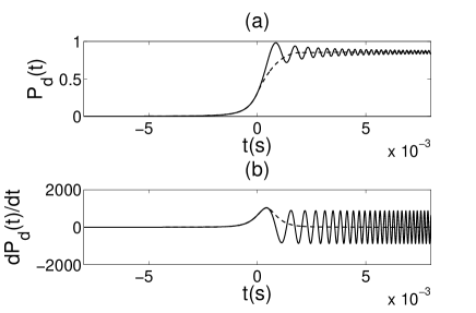
Figure 1: (a)The solid line is the time evolution of the probability function $P_{d}(t)$ and the dashed line is its step-like function fit. (b) The time derivative of the two functions in (a) and $\eta=0.2565$.

The time evolution of the probability function $P(t)$ can be found by numerically solving Eq.(1). A typical result of $P(t)$ is shown in Fig.1, where we see a sharp transition occurs around $t=0$ and is followed by decaying oscillations. This observation suggests an intuitive (or natural) definition for the LZ tunneling time. One may first fit the $P$ curve with a smooth step-like function (dashed line in Fig.1(a), and then define the half-width of its time derivative (dashed line in Fig.1(b)) as the tunneling time. However, like its counterpart in the wave packet and barrier system, this intuitive definition of tunneling time fails because of its two shortcomings. First, there are numerous methods to find the fitting step-like function in Fig.1(a); there is no obvious criterion by which one method is better than the other. Secondly, at the adiabatic limit, the $P$ curve looks drastically different from the typical case in Fig.1(a). As shown in Fig.2, the $P$ is a single-peaked function; one really has to be far-stretched to fit it with a step-like function. These two drawbacks show that this intuitive definition of the tunneling time based curve-fitting is not a good choice. One has to find an alternative.

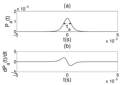
Figure 2: Time evolution of tunneling probability $P_{a}(t)$ and its time derivative $dP_{a}(t)/dt$ at the adiabatic limit. (a) The time evolution of the tunneling probability $P_{a}(t)$; (b) the function of $dP_{a}(t)/dt$, $\eta=0.10$.

In Ref.LZ5 , Vitanov introduced a general definition for the LZ tunneling time. His definition is

$$\tau=\frac{P(\infty)}{P^{{}^{\prime}}(0)}\,,$$ (4)

where the time derivative value $P^{{}^{\prime}}(0)$ at $t=0$ is used to represent the rate of the transition around $t=0$. For the typical time evolution of the probability function $P(t)$ shown in Fig.1, this definition works well. However, Vitanov’s definition fails at the adiabatic limit like the intuitive definition as we shall see later. In fact, Vitanov’s definition does not work in the adiabatic basis in general. A typical $P$ curve in the adiabatic basis is shown in Fig.3, where $P^{\prime}(0)$ clearly over-represents the transition rate.

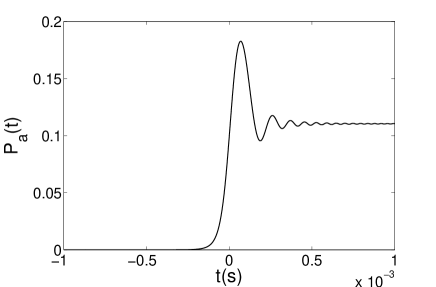
Figure 3: Time evolution of the tunneling probability in the adiabatic basis. $\eta=1.425$.

We overcome these difficulties and find a general definition of the tunneling time for the LZ model. In the definition, we first find a $t^{\prime}<0$ such that

$$P(t^{\prime})=\frac{1}{2}P_{max}\,,$$ (5)

where $P_{max}$ is the maximum value of $P$ when $t\leq 0$. Usually, $P_{max}=P(t=0)$. The above condition will be called half-width condition from now on for ease of reference. We then introduce two more variables

$$S_{1}= \int_{-\infty}^{0}\frac{d}{dt}P(t)dt=P(0)\,,$$ (6)

$$S_{2}= \int_{0}^{\infty}\frac{d}{dt}P(t)dt=P(\infty)-P(0)\,,$$ (7)

which are the left ($t<0$) area and right ($t>0$) area of the $dP/dt$ curve, respectively. With these defined variables, we define the tunneling time as

$$\tau=|t^{\prime}|(1+\Big{|}\frac{S_{2}}{S_{1}}\Big{|})\,.$$ (8)

Three quick remarks. i) The three variables in the definition can be computed without any ambiguity. ii) For the typical case shown in Fig.1, we have $S_{1}\approx S_{2}$ and, therefore, $\tau=2|t^{\prime}|$, which is in agreement of the “intuitive” definition that we discussed before. iii) The absolute value is used because $S_{2}$ can be negative in certain cases, for example, the case in Fig.2. The reason of the appearance of negative $S_{2}$ is that the transition around $t=0$ over-shoots the overall transition $P(\infty)-P(-\infty)$ and the system needs to spend some time to “wind back”.

In the following, we shall apply our definition and compute the tunneling times in the LZ model. Both analytical and numerical approaches will be used. The analytical approach is used for two limiting cases, the adiabatic limit and the sudden limit. For the LZ model, we can introduce a “quickness” parameter

$$\eta\equiv\frac{2\hbar\alpha}{\Delta^{2}}\,.$$ (9)

The adiabatic limit is $\eta\ll 1$ while $\eta\gg 1$ corresponds to the sudden limit. For a general case, we have to resort to the numerical method. We first solve numerically the equation of motion Eq.(1), then compute the tunneling probability function $P(t)$, and finally find the tunneling time with our definition in Eq.(8). In our computation, we use $\Delta=1.2\times 10^{-7}k_{b}$, where $k_{b}$ is Boltzmann constant, which is a typical value in molecular magnetapp .

The tunneling time will be computed in both the adiabatic basis and the diabatic basis. For clarity, we shall use $\tau_{d}$ for the tunneling time in the diabatic basis and $\tau_{a}$ for the tunneling time in the adiabatic basis.

III Tunneling Times In The Diabatic Basis

We first consider the diabatic basis and follow it with the discussion on the adiabatic basis in the next section.

III.1 Analytical results

At the adiabatic limit ($\eta\ll 1$), according to VitanovLZ5

$$P_{d}(t)\approx\frac{1}{2}+\frac{\alpha t}{2\sqrt{\alpha^{2}t^{2}+\Delta^{2}}}\,,$$ (10)

the variable $t^{\prime}$ can be obtained from the half-width condition

$$P_{d}(t)|_{t=t^{\prime}}=\frac{1}{2}(P_{d}(t\leq 0))_{max}=\frac{1}{4}\,.$$ (11)

The result is

$$t^{\prime}=-\frac{\sqrt{3}}{3}\frac{\Delta}{\alpha}\,.$$ (12)

Since we have $S_{1}=S_{2}$ for the tunneling curve Eq.(10), the tunneling time with our definition of Eq.(8) is

$$\tau^{a}_{d}=\frac{2\sqrt{3}}{3}\frac{\Delta}{\alpha}\,,$$ (13)

which agrees well with the result of Mullen et al.LZ8 .

At the sudden limit $\eta\gg 1$, it is beneficial to take a transformation

$$a(t) =\tilde{a}(t)\exp(-i\frac{\alpha t^{2}}{4\hbar})\,,$$ (14)

$$b(t) =\tilde{b}(t)\exp(i\frac{\alpha t^{2}}{4\hbar})\,,$$ (15)

for the LZ model. As a result, the diagonal terms in the Hamiltonian are transformed away and we can expand $\tilde{a}(t)$ and $\tilde{b}(t)$ in powers of $\eta$ (effectively, $\Delta$) LZ8 . For the initial condition $a(-\infty)=1$ and $b(-\infty)=0$, we obtain

$$a(t) =[1+\sum_{k=1}^{\infty}(-1)^{k}\frac{1}{(2\eta)^{k}}a_{2k}(y)]\exp(-i\frac{y^{2}}{4})\,,\quad$$ (16)

$$b(t) =[\sum_{k=1}^{\infty}(-1)^{k+1}\frac{1}{i(2\eta)^{k/2}}b_{2k-1}(y)]\exp(i\frac{y^{2}}{4})\,,\quad$$ (17)

where

$$a_{n}(y) =\int_{-\infty}^{y}\exp(ix_{1}^{2}/2)\int_{-\infty}^{x_{1}}\exp(-ix_{2}^{2}/2)\dots\int_{-\infty}^{x_{n-1}}\exp[(-1)^{n+1}ix_{n}^{2}/2]dx_{1}dx_{2}\dots dx_{n-1}dx_{n}\,,\quad$$ (18)

$$b_{n}(y) =\int_{-\infty}^{y}\exp(-ix_{1}^{2}/2)\int_{-\infty}^{x_{1}}\exp(ix_{2}^{2}/2)\dots\int_{-\infty}^{x_{n-1}}\exp[(-1)^{n}ix_{n}^{2}/2]dx_{1}dx_{2}\dots dx_{n-1}dx_{n}\,,\quad\raggedleft\@add@raggedleft$$ (19)

with $y=t/(\hbar/\alpha)^{1/2}$. At the sudden limit, it is sufficient to keep Eq.(17) to the lowest order of $1/\eta$. Consequently, we obtain

$$P_{d}(t) =|b(t)|^{2}\approx\bigg{|}\frac{1}{\sqrt{2\eta}}\int_{-\infty}^{y}\exp(-i\frac{x^{2}}{2})dx\bigg{|}^{2}$$ (20)

$$=\frac{1}{2\eta}\bigg{|}-\frac{\sqrt{2\pi}}{2}\exp(i\frac{3\pi}{4})+\int_{0}^{y}\exp(-i\frac{x^{2}}{2})dx\bigg{|}^{2}$$

$$=\frac{\pi}{2\eta}\Big{\{}\big{[}\frac{1}{2}+C(\frac{y}{\sqrt{\pi}})\big{]}^{2}+\big{[}\frac{1}{2}+S(\frac{y}{\sqrt{\pi}})\big{]}^{2}\Big{\}}^{2}\,,$$

where $C(y/\sqrt{\pi})$ and $S(y/\sqrt{\pi})$ are the Fresnel integralsFresnel . One can prove that the maximum value of $P_{d}$ for $t\leq 0$ is at $t=0$, where $P_{d}=\pi/(4\eta)$. Thus with the half-width condition

$$P_{d}(t^{\prime})=\frac{1}{2}P_{d}(0)=\frac{\pi}{8\eta}\,,$$ (21)

we find numerically that $t^{\prime}\approx-0.6241\sqrt{\frac{\hbar}{\alpha}}$. According to Refs.LZ1 ; LZ2 , we have

$$P_{d}(\infty)=1-\exp(-\frac{\pi}{\eta})\,.$$ (22)

Therefore, at the sudden limit ( $\eta\gg 1$), we have

$$\Big{|}\frac{S_{2}}{S_{1}}\Big{|}=\frac{P_{d}(\infty)-P_{d}(0)}{P_{d}(0)}\approx 3\,.$$ (23)

Based on our definition in Eq. (8), the tunneling time is

$$\tau^{s}_{d}\approx 4|t^{\prime}|=2.4964\sqrt{\frac{\hbar}{\alpha}},$$ (24)

which agrees well with the result of Mullen et al.LZ8 .

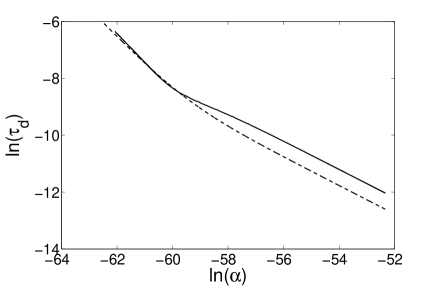
Figure 4: Tunneling times $\tau_{d}$ in the diabatic basis. The solid line is our numerical results and the dashed line is the empirical formula $\tau_{d}=\sqrt{\Delta^{2}/\alpha^{2}+2\hbar/\alpha}$ used in Ref.LZ4 . $\alpha$ is in the unit of $\frac{\Delta^{2}}{2\hbar}$.

III.2 Numerical results

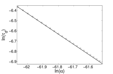
Figure 5: Tunneling time $\tau_{d}$ at the adiabatic limit in the diabatic basis. The circles are the theoretical results given in Eq.(13) and the solid line is the numerical results. $\alpha$ is in the unit of $\frac{\Delta^{2}}{2\hbar}$.

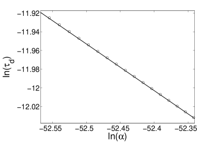
Figure 6: Tunneling time $\tau_{d}$ at the sudden limit in the diabatic basis. The circles are the theoretical results given in Eq.(24) and the solid line is the numerical results. $\alpha$ is in the unit of $\frac{\Delta^{2}}{2\hbar}$.

Our numerical results of the tunneling time $\tau_{d}$ in the diabatic basis is plotted in the log-log scale in Fig.4. In the figure, we see that the results for the two limiting cases are connected by a smooth kink. We have also compared these results with the empirical relation $\tau_{d}=\sqrt{\Delta^{2}/\alpha^{2}+2\hbar/\alpha}$ that was used in Ref.LZ4 ; the agreement is quite good.

We have amplified the results at the adiabatic and the sudden limits and plotted them in Fig.5. and Fig.6, respectively. In these two figures, we have also compared them to the analytical results and the agreement is excellent.

IV Tunneling Times In The Adiabatic Basis

As mentioned already, when one applies the LZ model to describe the tunneling between Bloch bands, it is more convenient to use the adiabatic basis. It turns out that the results in the adiabatic basis are quite different from the ones in the diabatic basis.

IV.1 Analytical results

As in the case of the diabatic basis, at the adiabatic limit($\eta\ll 1$), the tunneling probability function $P_{a}$ in the adiabatic basis has been found by Vitanov LZ5 ,

$$P_{a}(t)\approx\frac{\alpha^{2}\hbar^{2}\Delta^{2}}{4(\alpha^{2}t^{2}+\Delta^{2})^{3}}\,.$$ (25)

With the half-width condition,

$$P_{a}(t)|_{t=t^{\prime}}=\frac{1}{2}(P_{a}(t\leq 0))_{max}=\frac{\alpha^{2}\hbar^{2}}{8\Delta^{4}}\,,$$ (26)

we find that

$$t^{\prime}=-\sqrt{2^{1/3}-1}\frac{\Delta}{\alpha}\,.$$ (27)

Thus, based on our definition in Eq.(8), the tunneling time is

$$\tau^{a}_{a}=2\sqrt{2^{1/3}-1}\frac{\Delta}{\alpha}\,,$$ (28)

which is very similar to the tunneling time Eq.(13) in the diabatic basis. In contrast, according to Vitanov’s definition Eq.(4), the tunneling time isLZ5

$$\zeta_{a}^{a}=\frac{\sqrt{2}\Delta}{\sqrt{\alpha\hbar}}\exp(-\frac{\pi\Delta^{2}}{4\alpha\hbar})\,.$$ (29)

At the adiabatic limit ($\alpha\rightarrow 0$), the tunneling time $\zeta_{a}^{a}$ tends to be zero. This result contradicts with the physical reality, the tunneling time should be very long at the adiabatic limit. Thus, Vitanov’s definition does not work in this case. Alternatively, our result in Eq. (28) can be viewed as the first successful attempt to find the tunneling time at the adiabatic limit in the adiabatic basis.

We next consider the sudden limit ($\eta\gg 1$). In terms of $y=t/\sqrt{\hbar/\alpha}$, the instantaneous eigenstates of the Hamiltonian (2) are

$$\Phi(y)=\begin{pmatrix}c_{1}(y)\\ c_{2}(y)\end{pmatrix}=\begin{pmatrix}[\frac{1}{2}(1+\frac{y}{\sqrt{(y^{2}+2/\eta)}})]^{1/2}\\ [\frac{1}{2}(1-\frac{y}{\sqrt{(y^{2}+2/\eta)}})]^{1/2}\end{pmatrix}\,.$$ (30)

According to Eq. (16) and Eq. (17), we can obtain the tunneling probability up to the first order of $1/\eta$

$$P_{a}(y)\approx\bigg{|}{\begin{pmatrix}c_{1}(y)&c_{2}(y)\end{pmatrix}\begin{pmatrix}\exp(-i\frac{y^{2}}{4})\\ b_{1}(y)\exp(i\frac{y^{2}}{4})\end{pmatrix}}\bigg{|}^{2}\,.$$ (31)

With Eq.(19), we arrive at

$$P_{a}(y)\approx\frac{1}{2}+\frac{1}{2}\frac{y}{\sqrt{y^{2}+\frac{2}{\eta}}}-\frac{1}{\sqrt{\eta(\eta y^{2}+2)}}\cos\frac{y^{2}}{2}\int_{-\infty}^{y}\sin{\frac{x^{2}}{2}}dx+\frac{1}{2\eta}(\frac{1}{2}-\frac{1}{2}\frac{y}{\sqrt{y^{2}+\frac{2}{\eta}}})\,.$$ (32)

It is quite obvious that the last two terms of the above equation is much smaller than the first two terms. Finally, we obtain

$$P_{a}(t)\approx\frac{1}{2}+\frac{1}{2}\frac{\alpha t}{\sqrt{\alpha^{2}t^{2}+\Delta^{2}}}\,,\\$$ (33)

which is surprisingly identical to the result at the adiabatic limit in the diabatic basis (see Eq.(10)). As a result, we can similarly obtain the tunneling time

$$\tau^{s}_{a}=\frac{2\sqrt{3}}{3}\frac{\Delta}{\alpha}\,,$$ (34)

which agrees very well with Vitanov’s resultLZ5 .

IV.2 Numerical results

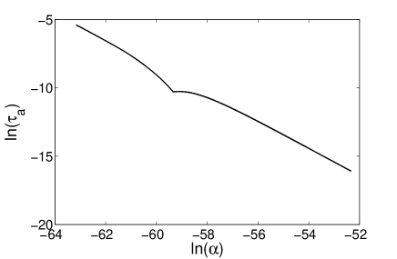
Figure 7: Tunneling time $\tau_{a}$ in the adiabatic basis, $\alpha$ is in the unit of $\frac{\Delta^{2}}{2\hbar}$.

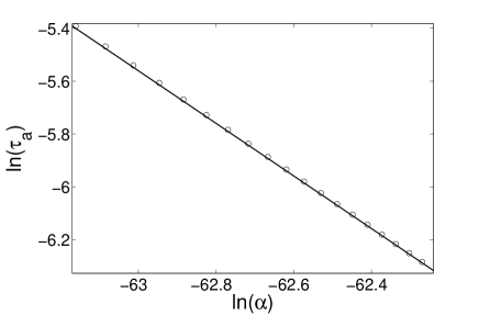
Figure 8: Tunneling time $\tau_{a}$ at the adiabatic limit in the adiabatic basis. The circles are the theoretical results given by Eq.(28); the solid line is the numerical results. $\alpha$ is in the unit of $\frac{\Delta^{2}}{2\hbar}$.

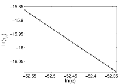
Figure 9: Tunneling time $\tau_{a}$ at the sudden limit in the adiabatic basis. The circles are the theoretical results given by Eq.(34); the solid line is the numerical results. $\alpha$ is in the unit of $\frac{\Delta^{2}}{2\hbar}$.

In the adiabatic basis, the numerical results of the tunneling time are shown in Fig.7. We see that the results in the two limiting cases are also connected by a kink. However, this kink is not as smooth as the kink in the diabatic basis; the first derivative of the tunneling time with respect to $\alpha$ is not continuous. The numerical results for the two limits, the adiabatic limit and the sudden limit, are plotted and compared to the theoretical results in Fig.8 and Fig.9, respectively. Again, we find an excellent agreement.

V DISCUSSION AND CONCLUSION

In the above, we have obtained analytical results for the tunneling times in the LZ model at two different limits and in two different bases. They are, respectively, $t_{d}^{a}$, $t_{d}^{s}$, $t_{a}^{a}$, and $t_{a}^{s}$. We have found that only $t_{d}^{s}$ is proportional to $\sqrt{\hbar/\alpha}$ while the rest of the three tunneling times all scale as $\Delta/\alpha$. It is not hard to understand why $t_{d}^{s}$, the tunneling time at the sudden limit and in the diabatic basis, does not scale as $\Delta/\alpha$. The effect of $\Delta$ is to couple the two bare states, $(1,0)$ and $(0,1)$. which serve as the base vectors in the diabatic basis. At the sudden limit, the system changes very fast and its wave function remains almost unchanged. As a result, the system does not feel the effect of $\Delta$. It is also not hard to understand that the two tunneling times at the adiabatic limit, $t_{a}^{a}$ and $t_{d}^{a}$, scale as $\Delta/\alpha$. At the adiabatic limit, the effect of $\Delta$ is fully felt by system and gets reflected in the tunneling time.

The most puzzling is $t_{a}^{s}$, the tunneling time at the sudden limit in the adiabatic basis. Unlike the other tunneling time $t_{d}^{s}$ at the sudden limit, it is proportional to $\Delta/\alpha$. Moreover, its corresponding probability function $P_{a}(t)$ described by Eq.(33) is surprisingly identical to the probability function $P_{d}(t)$ in Eq.(10), which is at the adiabatic limit in the diabatic basis. To understand this, we have to look into the details of the evolution. At the adiabatic limit, the system follows its instantaneous eigenstate as demanded by the quantum adiabatic theoremqat . $P_{d}(t)$ in Eq.(10) is obtained by projecting this instantaneous eigenstate to the bare state $(0,1)$. At the sudden limit, the wave function of the system changes little and remains in the bare state $(1,0)$. However, in the adiabatic basis, this wave function needs to be projected to the instantaneous eigenstate to obtain $P_{a}(t)$ described by Eq.(33). As we know, projecting a bare state to an instantaneous eigenstate is the identical to projecting the same instantaneous eigenstate to the same bare state. This explains why the probability function $P_{a}(t)$ in Eq.(33) is the same as $P_{d}(t)$ in Eq.(10). Consequently, this also explains why $t_{a}^{s}$ scales as $\Delta/\alpha$.

In sum, we have presented a general definition of the tunneling time for the Landau-Zener model. We have shown that this definition works for any sweeping rate and can be used for the numerical computation of the tunneling time without any ambiguity. In particular, we have obtained analytical results for the two limiting cases, the adiabatic limit and the sudden limit. We have not only reproduced known results but also found the tunneling time at the adiabatic limit in the adiabatic basis, which has not been found before to our knowledge.

VI Acknowledgements

This work was supported by the NSF of China (10504040, 10825417) and the 973 project of China (2005CB724500, 2006CB921400).

References

- (1) H. Frauenfelder and P. G. Wolynes, Science 229, 337 (1985).
- (2) A. Garg, J. N. Onuchi, and V. Ambegaokar, J. Chem. Phys. 83, 4491 (1985).
- (3) J. J. Hopfield, Proc. Natl. Acad. Sci. U.S.A 71, 3640 (1974).
- (4) See, for example, E. E. Nikitin and S. Ya. Umanskii, Theory of Slow Atomic Collisions (Spring-Verlag, Berlin 1984); A. Yoshimori and K. Makoshi, Prog. Surf. Sci. 21, 251 (1986).
- (5) Leavens, C. R., and G. C. Aers, in Scanning Tunneling Microscopy III, edited by R. Wiesendanger and H-J. Güntherodt (Springer, New York, 1993).
- (6) Sokolovski, D., and L. M. Baskin, Phys. Rev. A 36, 4604 (1987).
- (7) Jensen, K, L., and F. Buot, Appl, Phys. Lett. 55, 669 (1989).
- (8) J. Liu, L. F., B. Y. Ou, and S. G. Chen, Dae-II Choi, B. Wu and Q. Niu, Phys. Rev. A 66, 023404 (2002).
- (9) J. Liu, B. Wu and Q. Niu, Phys. Rev. Lett. 90, 170404 (2003).
- (10) D. F. Ye, L. B. Fu, and J. Liu, Phys. Rev. A 77, 013402 (2008).
- (11) G. F. Wang, D. F. Ye, L. B. Fu, X. Z. Chen and J. Liu, Phys. Rev. A 74, 033414 (2006).
- (12) W. Wernsdorfer, R. Sessoli, A. Caneschi, D. Gatteschi, A. Cornia, and D. Mailly, J. Appl. Phys. 87, 5481 (2000).
- (13) R. Landauer, Nature 341, 567 (1989).
- (14) Th. Martin and R. Landauer, Phys. Rev. A 47, 2023 (1993).
- (15) A. Peres, Am. J. Phys. 7, 48 (1980).
- (16) M. Büttiker and R. Landauer, Phys. Rev. Lett. 49, 1739 (1982).
- (17) D. Sokolovski and L. M. Baskin, Phys. Rev. A 36, 4604 (1987).
- (18) Q. Niu and M. G. Raizen, Phys. Rev. Lett. 80, 3491 (1998).
- (19) R. Landauer and Th. Martin, Solid State Commun. 84, 115 (1992).
- (20) R. Landauer and Th. Martin, Rev. Mod. Phys. 66, 217 (1994).
- (21) L. D. Landau, Phys. Z. Sowjetunion 2, 46 (1932).
- (22) C. Zener, Proc. R. Soc. London, Ser. A 137, 696 (1932).
- (23) K. Mullen, E. Ben-Jacob, Y. Gefen and Z. Schuss, Phys. Rev. Lett. 62, 2543 (1989).
- (24) N. V. Vitanov, Phys. Rev. A 59, 988 (1999); N. V. Vitanov and B. M. Garraway, Phys. Rev. A 53, 4288 (1996).
- (25) J. Liu, B. Wu, L. Fu, R. B. Diener. and Q. Niu, Phys. Rev. B 65, 224401 (2002).
- (26) B. Wu and Q. Niu, Phys. Rev. A 61, 023402 (2000).
- (27) M. Abramowitz and T. A. Stegun, Handbook of mathematical functions - with formulas, graphs, and mathematical tables (Dover, New York, 1970).
- (28) A. Messiah, Quantum Mechanics (Dover, New York, 1999).