Thermodynamic potential of a mechanical constitutive model for two-phase band flow

Abstract

Starting from a simple mechanical constitutive model (the non-local diffusive Johnson-Segalman model; DJS model), we provide a rigorous theoretical explanation as to why a unique value of the stress plateau of a highly sheared viscoelastic fluid is stably realized. The present analysis is based on a reduction theory of the degrees of freedom of the model equation in the neighborhood of a critical point, which leads to a time-evolution equation that is equivalent to those for first-order phase transitions.

PACS numbers: 47.50.-d, 47.20.Ft, 47.54.-r

Highly sheared viscoelastic fluids are known to have spatially inhomogeneous structures, i.e., ”shear bands” kn:Hoffmann ; kn:review-of-Cates , where the fluid is separated into two regions with different values of the velocity gradient. In this phenomenon, a stress plateau is observed in the stress-strain curve (SS curve).

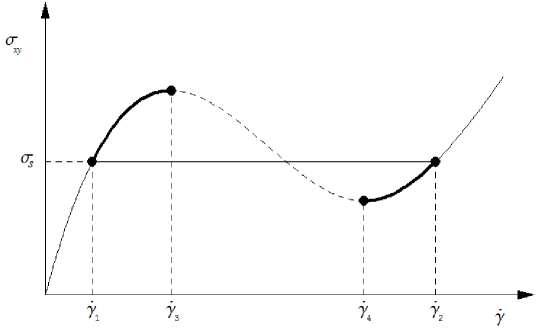
Figure 1: Figure 1: Schematic representation of shear banding. In the regions of shear rate where the SS curve has a positive slope, $\dot{\gamma}_{1}<\dot{\gamma}<\dot{\gamma}_{3}$, and $\dot{\gamma}_{4}<\dot{\gamma}<\dot{\gamma}_{2}$, both the homogeneous flow and banded flow are stable. Hence, in order to determine which state is finally realized in these regions, it is necessary to have some evaluation function to compare the stabilities of these states.

This phenomenon has been explained using an N-shaped SS curve, as depicted in Fig. 1 cates-mcleish . In the region of the shear rate where the SS curve has a negative slope (referred to hereafter as the negative-slope region), the uniform flow is unstable, and then the fluid separates into two stable domains having two unique values of shear rates, denoted by $\dot{\gamma}_{1}$ and $\dot{\gamma}_{2}$ ($\dot{\gamma}_{1}<\dot{\gamma}_{2}$). As the applied shear rate $\dot{\gamma}$ increases, the relative volume fraction of the domain with $\dot{\gamma}_{2}$ increases. This scenario enables us to explain the appearance of the shear stress plateau using a consideration similar to thermodynamics. The validity of this scenario has been generally confirmed by direct experimental observations kn:birefringence ; kn:NMR ; kn:light-scattering .

On the other hand, there are some theoretical disadvantages associated with this scenario. One such disadvantage is the fact that the origin of the unique value of the stress plateau, $\sigma_{s}$, is unknown. (In experiments, the value of the stress plateau is known to be uniquely determined independently of the flow history.) A solution to this problem is given by adding a non-local term (a diffusion term) to the constitutive model. In References kn:yuan-Europhys ; kn:Lu ; kn:Fielding the uniqueness of the value of $\sigma_{s}$ is demonstrated numerically, and in Reference Dhont a selection rule for $\sigma_{s}$, which is analogous to the Maxwell equal area construction, is provided analytically.

Although the problem of the unique determination of $\sigma_{s}$ was proven in the above references, another important problem remains, i.e., the global stability of the banded state. As stated above, in the negative-slope region the banded state is finally realized because of the instability of the homogeneous flow. However, in the remaining regions, (a)-(c) and (d)-(b) as indicated in Fig. 1, the SS curve has a positive slope and so the homogeneous flow is stable (at least locally). Thus, it is not guaranteed that the banded state is finally realized in these regions. In other words, we cannot determine whether the homogeneous flow or the banded flow is more stable. This is because we have not yet had an evaluation function such as a thermodynamic potential for the models describing the shear banding.

In the present article, we will demonstrate the metastability of the above-mentioned homogeneous flow by deriving an evaluation function from a simple mechanical model, called Johnson-Segalman (JS) equation with a diffusion term (DJS equation). The DJS model is a widely accepted model as a paradigm of shear banding, with which characteristic experimental results are well reproduced numerically kn:yuan-Europhys ; kn:Lu ; kn:Fielding . Here, the term ”mechanical” indicates that the model is constructed in a purely mechanical manner, i.e., the model does not have an explicit thermodynamic potential. While there are some other extended models on shear bands doi-onuki ; kn:coupling-model-yuan ; kn:Fielding-Olmsted-2003 , as a first trial on this issue we will adopt the simplest DJS equation. In fact, the method we use in the present study, which is based on the reduction theory developed in the field of non-linear dynamics kn:kuramoto-book , is also applicable to a wide class of models.

We start with the following governing equations for a viscoelastic fluid:

$$\nabla\cdot\boldsymbol{v}\!\!\! = \!\!\!0,$$ (1)

$$\rho(\frac{\partial}{\partial t}+\boldsymbol{v}\cdot\nabla)\boldsymbol{v}\!\!\! = \!\!\!\nabla\cdot(\boldsymbol{\Sigma}+2\eta\boldsymbol{D}-p\boldsymbol{I}),$$ (2)

$$(\frac{\partial}{\partial t}+\boldsymbol{v}\cdot\nabla)\boldsymbol{\Sigma}\!\!\! = \!\!\!a(\boldsymbol{D}\cdot\boldsymbol{\Sigma}+\boldsymbol{\Sigma}\cdot\boldsymbol{D})+(\boldsymbol{\Omega}\cdot\boldsymbol{\Sigma}-\boldsymbol{\Sigma}\cdot\boldsymbol{\Omega})+2G\boldsymbol{D}-\frac{\boldsymbol{\Sigma}}{\tau}-2D_{0}\nabla^{2}\boldsymbol{D}.$$ (3)

Equation (1) represents the incompressibility condition of the fluid, where $\boldsymbol{v}$ is the fluid velocity. This condition holds in usual fluids and guarantees that the density $\rho$ is constant throughout the fluid. Equation (2) represents the momentum balance of the fluid, where the total stress tensor denoted by $\boldsymbol{\sigma}$ is assumed to be composed of two contributions as $\boldsymbol{\sigma}=\boldsymbol{\Sigma}+2\eta\boldsymbol{D},$ where $\boldsymbol{\Sigma}$ is the contribution from the polymeric components and $2\eta\boldsymbol{D}$ is the contribution from the solvent. We assume that the polymeric component $\boldsymbol{\Sigma}$ obeys the DJS equation given by Eq. (3), while the solvent is assumed to be a Newtonian fluid so that its contribution is a product of the viscosity $\eta$ and the symmetric part of the velocity gradient tensor $\boldsymbol{D}=((\nabla\boldsymbol{v})^{T}+\nabla\boldsymbol{v})/2$. The quantity $p$ is the pressure, and $\boldsymbol{I}$ is the unit tensor. Equation (3) is the DJS equation, where $a$ is a parameter that satisfies $0\leq a\leq 1$. This parameter $a$ is called the ”slip parameter”, which represents the degree of non-affine deformation under the flow kn:original-JS-equation . $\boldsymbol{\Omega}$ is the antisymmetric part of the velocity gradient tensor, defined by $\boldsymbol{\Omega}=((\nabla\boldsymbol{v})^{T}-\nabla\boldsymbol{v})/2$. The coefficients $G$, $\tau$ and $D_{0}$ in Eq. (3) are scalar constants having the dimensions of stress, time, and (stress $\times$ (length)²), respectively. The last term $\nabla^{2}\boldsymbol{D}$ is the diffusive stress term, the components of which are $\sum_{i}{\partial}^{2}D_{jk}/\partial x_{i}^{2}$ for any $j$ and $k$. In References kn:Lu ; kn:Fielding , the non-local term of the DJS equation is assumed to have the form $\nabla^{2}\boldsymbol{\Sigma}$. The physical meaning of this form can be understood as a diffusion of the stress tensor originating from the diffusive flux of the polymeric components. Although the physical meaning of $\nabla^{2}\boldsymbol{D}$ appears to be less obvious, it will be shown that the final results of the present analysis are unchanged both of these choices. (See the last paragraph of this article.)

Using this setup, we consider a one-dimensional simple shear flow, i.e., a flow contained between two parallel plates moving with a constant relative speed $v_{0}$ along the $x$-axis. The velocity distribution of the fluid $\boldsymbol{v}\equiv(v_{x},v_{y},v_{z})$ in such a situation is given as $v_{x}=v_{x}(y,t)$ $v_{y}=v_{z}=0$ with the boundary conditions $v_{x}(0,t)=0$ and $v_{x}(L,t)=v_{0}$ for any time $t$, where $L$ is the distance between the two plates. For the solvability of the model, we need additional boundary conditions. We require ${\partial}^{2}v_{x}(y,t)/\partial y^{2}|_{y=0,L}=0$ for any time $t$. This boundary condition corresponds to the situation in which the polymeric components are impenetrable at the walls of the plates kn:meaning-of-diffusion-term ; kn:meaning-of-diffusion-term-olmsted .

To simplify the equations, we use the same non-dimensionalization procedure introduced in early investigations kn:nondimensionalization ; kn:Lu , i.e., $t/\tau\rightarrow t$, $y/L\rightarrow y$, $\rho L^{2}/\tau^{2}G\rightarrow\rho$, $\eta/G\tau\rightarrow\eta$ and $D_{0}/2GL^{2}\rightarrow D_{1}$. By applying this non-dimensionalization, we obtain three non-dimensional quantities, $\kappa(y,t)$, $N(y,t)$ and $S(y,t)$, defined by $\kappa\equiv\sqrt{1-a^{2}}\tau\frac{\partial v_{x}}{\partial y}$, ${N}\equiv[(1-a)\Sigma_{xx}-(1+a)\Sigma_{yy}]/2G$, and ${S}\equiv\sqrt{1-a^{2}}\Sigma_{xy}/G$. Then, Eqs. (1)-(3) reduce to the following set of equations for $\kappa$, $N$ and $S$:

$$\frac{\partial{\kappa}}{\partial{t}}\!\!\! = \!\!\!\frac{1}{{\rho}}\frac{\partial{}^{2}}{\partial{y}^{2}}({S}+{\eta}{\kappa}),$$ (4)

$$\frac{\partial{N}}{\partial{t}}\!\!\! = \!\!\!{\kappa}{S}-{N},$$ (5)

$$\frac{\partial{S}}{\partial{t}}\!\!\! = \!\!\!-{\kappa}{N}+{\kappa}-{S}-D_{1}\frac{\partial{}^{2}}{\partial{y}^{2}}{\kappa}.$$ (6)

. Here, Eq. (4) is obtained by differentiating the $x$-component of both sides of Eq. (2) and eliminating $v_{x}$. In this non-dimensional system, the boundary conditions are given as

$$\int_{0}^{1}{\kappa}({y},t)d{y}=\bar{\kappa}\qquad\mbox{and}\qquad\left.\frac{\partial\kappa({y},t)}{\partial{y}}\right|_{{y}=0,1}=0,$$ (7)

where $\bar{\kappa}$ is a constant given by $\bar{\kappa}=\tau\sqrt{1-a^{2}}v_{0}/L$. In the following analysis, we assume that the quantity $D_{1}$ is an extremely small positive number compared to unity, which may be justified by the fact that $D_{1}\propto 1/L^{2}$. This assumption corresponds to the situation in which the width of the interface between the shear bands is much smaller than the system size because in this model the width of the interface is given by a quantity proportional to $\sqrt{D_{1}}$.

A trivial $y$-independent stationary solution of Eqs. (4)-(6) that satisfies the boundary conditions of Eqs. (7) is $\kappa=\bar{\kappa}$, $N=\bar{\kappa}^{2}/(1+\bar{\kappa}^{2})$, and $S=\bar{\kappa}/(1+\bar{\kappa}^{2})$. This solution gives a trivial value of the total stationary shear stress $\bar{\sigma}=\frac{\bar{\kappa}}{(1+\bar{\kappa}^{2})}+\eta\bar{\kappa}$. When $\eta>1/8$, $\bar{\sigma}$ is a monotonic function of $\bar{\kappa}$, and when $\eta<1/8$, $\bar{\sigma}$ is a non-monotonic N-shaped function of $\bar{\kappa}$ that has a region with a negative slope. The negative-slope region of the DJS equation is given by $\kappa_{n-}<\bar{\kappa}<\kappa_{n+}$ with $\kappa_{n\pm}=\sqrt{-1+\frac{1}{2\eta}\pm\frac{\sqrt{1-8\eta}}{2\eta}}$. The trivial stationary solutions have been proven to be unstable in this region kn:unstable ; kn:unstable-yuan . When $\eta$ approaches $1/8$, the negative-slope region $(\kappa_{n-},\kappa_{n+})$ converges to a single point $\bar{\kappa}=\sqrt{3}$, which allows us to define the “critical point” of the DJS equation as $({\bar{\kappa}}^{*},\eta^{*})=(\sqrt{3},1/8)$. At this critical point, the conditions $d\bar{\sigma}/d\bar{\kappa}|_{\bar{\kappa}={\bar{\kappa}}^{*}}=0$ and $d^{2}\bar{\sigma}/d\bar{\kappa}^{2}|_{\bar{\kappa}={\bar{\kappa}}^{*}}=0$ hold simultaneously.

A non-trivial stationary solution of Eqs.(4)-(6) in the negative-slope region for $\eta<1/8$ is obtained in the case with the $\nabla^{2}\boldsymbol{D}$ term in Eq. (3). By assuming a stationary solution of Eqs.(4)-(6) under the boundary condition $v(y,t)|_{y=0,L}=const$, we obtain

$$\kappa(1-\kappa(\sigma_{s}-\eta\kappa))-(\sigma_{s}-\eta\kappa)-D_{1}\frac{d^{2}\kappa}{dy^{2}}=0.$$ (8)

We can identify this equation with an equation of motion for a particle with position $\kappa$ at time $y$ moving in a quartic potential. This equation has a non-trivial solution that satisfies the boundary conditions Eq.(7) only when

$$\sigma_{s}=3\sqrt{-\eta^{2}+\frac{\eta}{2}}.$$ (9)

Note that this value of $\sigma_{s}$ does not depend on $\bar{\kappa}$. At this value of $\sigma_{s}$, the non-trivial solution of Eq. (8) is given as

$$\kappa(y)=\kappa_{0}(y)\equiv\frac{\kappa_{+}-\kappa_{-}}{2}\tanh\left[\frac{y-\displaystyle\frac{\kappa_{+}-\bar{\kappa}}{\kappa_{+}-\kappa_{-}}}{\displaystyle\xi}\right]+\frac{\kappa_{+}+\kappa_{-}}{2},$$ (10)

, where $\kappa_{\pm}=\frac{\sqrt{\frac{1}{\eta}-2}\pm\sqrt{\frac{1}{\eta}-8}}{\sqrt{2}}$. This non-uniform solution describes a shear banding, in which the relative volume fraction of the regions with lower shear rate is given by $(\kappa_{+}-\bar{\kappa})/(\kappa_{+}-\kappa_{-})$ and the width of the interface between different regions is given by $\xi\equiv\sqrt{D_{1}/(1-8\eta)}$. From the symmetry of Eq.(8), we know that $\kappa(y)=\kappa_{0}(1-y)$ is also a non-uniform solution of Eq. (8). It is worth noting that the analytical results of Eqs.(9) and (10) are in good agreement with the numerical results for the same model kn:yuan-Europhys .

As mentioned in the introduction, a linear stability analysis shows that the trivial homogeneous solution is unstable in the negative-slope region ($\kappa_{n-}<\kappa<\kappa_{n+}$), and therefore a nontrivial solution should emerge. However, in the remaining regions ($\kappa_{-}<\kappa<\kappa_{n-}$ and $\kappa_{n+}<\kappa<\kappa_{+}$), where $\bar{\sigma}$ has a positive slope, there is no guarantee that the non-trivial solution is finally realized because the homogeneous flow is still stable (at least locally) in these regions. Therefore, for a complete understanding of the stress plateau, it is not sufficient to determine the value of $\sigma_{s}$ uniquely and obtain the corresponding non-trivial solution. The metastability of the homogeneous flow in the positive-slope regions must be demonstrated. To do this, we shall reduce the DJS equation in the neighborhood of its critical point.

The reduction procedure is as follows. First, we ignore the inertia term (the adiabatic approximation) in Eq. (4) because the Reynolds number is small for usual viscoelastic fluid flows. We then have an approximate expression for $\kappa$ as $\kappa(y,t)\simeq\bar{\kappa}-e(S-S_{0}),$ where $e=1/\eta$, and $S_{0}$ is the mean value of $S$ over the spatial coordinate $y$, i.e., $S_{0}(t)=\int_{0}^{1}S(y,t)dy$. Substituting this approximate expression for $\kappa$ into Eqs.(5) and (6) yields

$$\frac{\partial N}{\partial t}\!\!\! = \!\!\!(\bar{\kappa}-e(S-S_{0}))S-N,$$ (11)

$$\frac{\partial S}{\partial t}\!\!\! = \!\!\!(\bar{\kappa}-e(S-S_{0}))(1-N)-S+d\frac{\partial{}^{2}S}{\partial y^{2}},$$ (12)

where $d=D_{1}e$. Next, in order to clarify which mode is dominant in the critical region, we carry out a linear stability analysis at the critical point $(\bar{\kappa}^{*},e^{*})=(\sqrt{3},8)$. Linearizing Eqs.(11) and (12) with respect to the stationary solution at the critical point, $({\bar{N}}^{*},{\bar{S}}^{*})=(3/4,\sqrt{3}/4)$, in terms of the deviations $s_{0}$, $n_{0}$, $\hat{s}$, and $\hat{n}$ defined by $s_{0}=\int_{0}^{1}(S-{\bar{S}}^{*})dy$, $n_{0}=\int_{0}^{1}(N-{\bar{N}}^{*})dy$, $\hat{s}=S-{\bar{S}}^{*}-s_{0}$, and $\hat{n}=N-{\bar{N}}^{*}-n_{0}$, we have

$$\left\{\begin{split}\frac{\partial n_{0}}{\partial t}&=-n_{0}+\sqrt{3}s_{0}\\ \frac{\partial s_{0}}{\partial t}&=-\sqrt{3}n_{0}-s_{0}\end{split}\right.\hskip 85.35826pt\left\{\begin{split}\frac{\partial\hat{n}}{\partial t}&=-\hat{n}-\sqrt{3}\hat{s}\\ \frac{\partial\hat{s}}{\partial t}&=-\sqrt{3}\hat{n}-3\hat{s}.\end{split}\right.$$ (13)

Here, we have neglected the diffusion term because, according to the reduction theory for partial differential equations, the diffusion term should be regarded as a small perturbation to the uniform system kn:kuramoto-book . The eigenvalues of the former set of equations are $-1\pm i\sqrt{3}$, and those for the latter set of equations are $0$ and $-4$. The corresponding eigenmodes of the latter set of equations are

$$\phi\!\!\! = \!\!\!\frac{1}{2}(-\sqrt{3}\hat{n}+\hat{s}),$$ (14)

$$\psi\!\!\! = \!\!\!\frac{1}{2}(\hat{n}+\sqrt{3}\hat{s}),$$ (15)

respectively. Thus, we find that, in the vicinity of the critical point, the variable $\phi$ is the unique slow one of the system and the other variables $n_{0}$, $s_{0}$ and $\psi$ are solved by $\phi$ kn:kuramoto-book ; kn:Haken-book . Based on this observation, we first rewrite the original Eqs.(11) and (12) in terms of $n_{0}$, $s_{0}$, $\phi$ and $\psi$ as

$$\frac{\partial n_{0}}{\partial t}\!\!\! = \!\!\!{\bar{S}}^{*}(\bar{\kappa}-{\bar{\kappa}}^{*})-n_{0}+\bar{\kappa}s_{0}-\frac{e}{4}\langle(\phi+\sqrt{3}\psi)^{2}\rangle,$$ (16)

$$\frac{\partial s_{0}}{\partial t}\!\!\! = \!\!\!(\bar{\kappa}-{\bar{\kappa}}^{*})(1-{\bar{N}}^{*})-\bar{\kappa}n_{0}-s_{0}+\frac{e}{4}\langle(-\sqrt{3}\phi+\psi)(\phi+\sqrt{3}\psi)\rangle,$$ (17)

$$\frac{\partial\phi}{\partial t}\!\!\! = \!\!\!\frac{1}{2}(-\sqrt{3}f_{1}+f_{2})+\frac{d}{4}\partial_{y}^{2}(\phi+\sqrt{3}\psi),$$ (18)

$$\frac{\partial\psi}{\partial t}\!\!\! = \!\!\!\frac{1}{2}(f_{1}+\sqrt{3}f_{2})+\frac{\sqrt{3}d}{4}\partial_{y}^{2}(\phi+\sqrt{3}\psi),$$ (19)

where the bracket denotes an integral over the entire domain of $y$, i.e., $\langle\cdot\rangle=\int_{0}^{1}\cdot dy$. The quantities $f_{1}$ and $f_{2}$ are functionals of $n_{0}$, $s_{0}$, $\phi$, and $\psi$, defined by $f_{1}=\{-\hat{n}+(-e{\bar{S}}^{*}+\bar{\kappa})\hat{s}-es_{0}\hat{s}-e(\hat{s}^{2}-\langle\hat{s}^{2}\rangle)\}|_{p}$ and $f_{2}=\{-\bar{\kappa}\hat{n}-(e(1-{\bar{N}}^{*})+1)\hat{s}+en_{0}\hat{s}+e(\hat{n}\hat{s}-\langle\hat{n}\hat{s}\rangle)\}|_{p}$, where the subscript $p$ indicates the substitutions $\hat{n}=\frac{1}{2}(-\sqrt{3}\phi+\psi)$ and $\hat{s}=\frac{1}{2}(\phi+\sqrt{3}\psi)$ in each expression. Note that these Eqs.(16)-(19) are still equivalent to the original Eqs.(11) and (12). Next, we assume that the variables $n_{0}$, $s_{0}$, and $\psi$ are functionals of $\phi$ and functions of $y$, denoted by $n_{0}[\phi,y]$, $s_{0}[\phi,y]$ and $\psi[\phi,y]$, and define a functional $G[\phi,y]$ as the right-hand side of Eq.(18). Substituting these forms into Eqs. (16)-(19) gives four algebraic equations for $n_{0}$, $s_{0}$, $\psi$, and $G$ with independent variables $\phi$ and $y$. Here, our task is reduced to determining the forms of these four functionals. Introducing two small parameters $k$ and $\epsilon$ defined as $k=\bar{\kappa}-{\bar{\kappa}}^{*}$ and $\epsilon=e-e^{*}$, ($|\epsilon|\ll 1$, $|k|\ll 1$) and realizing that the difference between the shear rates of each domain is on the order $O(\sqrt{\epsilon})$ $(\epsilon>0)$, which is known from the expanded form of $\bar{\sigma}$ near the critical point, we can proceed to the perturbative calculation systematically. The results are $n_{0}=\frac{\sqrt{3}}{8}k-\frac{k^{2}}{8}-2\langle\phi^{2}\rangle$, $s_{0}=-\frac{k}{8}$, $\psi=\frac{k\phi}{2}-(\phi^{2}-\langle\phi^{2}\rangle)$ and $G=(\frac{\epsilon}{8}-\frac{3}{4}k^{2})\phi+3k(\phi^{2}-\langle\phi^{2}\rangle)-4(\phi^{3}-\langle\phi^{3}\rangle)$. Here we have used the property $\langle\phi\rangle=0$, which results from its definition (14). In the above calculation, we have neglected the diffusion terms because of the smallness of $d$. If we retain the diffusion terms up to the lowest order in $d$, we have the following time evolution equation for $\phi$:

$$\frac{\partial\phi}{\partial t}=(\frac{\epsilon}{8}-\frac{3}{4}k^{2})\phi+3k(\phi^{2}-\langle\phi^{2}\rangle)-4(\phi^{3}-\langle\phi^{3}\rangle)+\frac{d}{4}\frac{\partial{}^{2}\phi}{\partial y^{2}}.$$ (20)

This equation expresses the main result of the present research. The dynamic variable $\phi$ is essentially an “order parameter” that which measures the inhomogeneity of the viscoelastic stress field and includes the contributions from both the shear stress and the first normal stress difference. Equation (20) has the same form as that of the time-dependent Ginzburg-Landau (TDGL) equation for first-order phase transitions in thermodynamics kn:landau-book ; kn:book-ohta . A non-trivial stationary solution of Eq. (20) for $\epsilon>0$ is readily obtained, which is consistent with the exact solution of Eq. (10) to the lowest order in $\epsilon$. An important advantage of the reduced equation, Eq. (20) is that we are able to prove the metastability of the homogeneous flow, which is readily performed by conventional means, e.g., a common tangent construction. A detailed discussion on the properties of Eq. (20) will be reported in a future paper kn:in-preparation .

Finally, we would like to comment on our choice of the diffusion term. In Eq. (3), even if we replace the diffusion term $D_{0}\nabla^{2}\boldsymbol{D}$ with the usual form $D_{2}\nabla^{2}\boldsymbol{\Sigma}$, the reduced TDGL-type equations is unchanged. The only difference is the diffusion constant appearing in (20), where $d/4$ is replaced by $\tau D_{2}/L^{2}$.

References

- (1) H. Rehage and H. Hoffmann, J. Phys. Chem. 92, 4712 (1988); Mol. Phys. 74, 933 (1991).
- (2) M. E. Cates and M. Fielding, Adv. Phys. 55, 799 (2006).
- (3) N. A. Spenley, M. E. Cates, and T. C. McLeish, Phys. Rev. Lett. 71, 939 (1993).
- (4) J. P. Decruppe , R. Cressely, R. Makhloufi, and E. Cappelaere, Colloid Polym. Sci. 273, 346 (1995).
- (5) R. W. Mair, and P. T. Callaghan, Europhys. Lett. 36, 719 (1996); E. Fischer and P. T. Callaghan, Phys. Rev. E 64, 011501 (2001).
- (6) S. Lerouge, J. P. Decruppe, and C. Humbert, Phys. Rev. Lett. 81, 5457 (1998).
- (7) X. F. Yuan, Europhys. Lett. 46, 542 (1999).
- (8) C. Y. D. Lu, P. D. Olmsted, and R. C. Ball, Phys. Rev. Lett. 84, 642 (2000).
- (9) S. M. Fielding, Phys. Rev. Lett. 95, 134501 (2005).
- (10) J. K. G. Dhont, Phys. Rev. E 60, 4534 (1999).
- (11) M. Doi and A. Onuki, J. Phys. II France 2, 1631 (1992).
- (12) X. F. Yuan and L. Jupp, Europhys. Lett. 60, 691 (2002).
- (13) S. M. Fielding and P. D. Olmsted, Phys. Rev. Lett. 90, 224501 (2003).
- (14) M. Johnson and D. Segalman, J. Non-Newtonian Fluid Mech. 2, 255 (1977).
- (15) A. W. El-Kareh and L. G. Leal, J. Non-Newtonian Fluid Mech. 33, 257 (1989).
- (16) P. D. Olmsted, O. Radulescu, and C. Y. D. Lu, J. Rheol. 44, 257 (2000).
- (17) D. S. Malkus, J. A. Nohel, and B. J. Plohr, J. Comput. Phys. 87, 464 (1990).
- (18) J. Yerushalmi, S. Katz, and R. Shinnar, Chem. Eng. Sci. 25, 1891 (1970).
- (19) P. Espanol, X. F. Yuan, and R. C. Ball, Non-Newtonian Fluid Mech. 65, 93 (1996).
- (20) H. Mori and Y. Kuramoto, Dissipative Structures and Chaos (Springer-Verlag, Berlin, 1998).
- (21) H. Haken, Advanced Synergetics: Instability Hierarchies of Self-Organizing Systems and Devices (Springer-Verlag, Berlin, 1983).
- (22) L. D. Landau and E. M. Lifshitz, Statistical Physics (Pergamon Press, Oxford, 1980).
- (23) Kyozi Kawasaki, Masuo Suzuki and Akira Onuki (editors), Formation, dynamics and statistics of patterns (Teaneck, N.J.: World Scientific, Singapore, 1990).
- (24) K. Sato, X. F. Yuan, and T. Kawakatsu, in preparation.