A comparative study of dynamical simulation methods for the dissociation of molecular Bose-Einstein condensates

Abstract

We describe a pairing mean-field theory related to the Hartree-Fock-Bogoliubov approach, and apply it to the dynamics of dissociation of a molecular Bose-Einstein condensate (BEC) into correlated bosonic atom pairs. We also perform the same simulation using two stochastic phase-space techniques for quantum dynamics — the positive $P$-representation method and the truncated Wigner method. By comparing the results of our calculations we are able to assess the relative strength of these theoretical techniques in describing molecular dissociation in one spatial dimension. An important aspect of our analysis is the inclusion of atom-atom interactions which can be problematic for the positive-$P$ method. We find that the truncated Wigner method mostly agrees with the positive-$P$ simulations, but can be simulated for significantly longer times. The pairing mean-field theory results diverge from the quantum dynamical methods after relatively short times.

I Introduction

The dissociation of a molecular Bose-Einstein condensate (BEC) Thompson et al. (2005); Greiner et al. (2005); D$\ddot{\textnormal{u}}$rr et al. (2004); Mukaiyama et al. (2004) into correlated atom pairs is a process analogous to parametric down-conversion in optics. Down-conversion involving photons has been pivotal in the advancement of quantum optics by allowing for the generation of strongly entangled states. In the same way, molecular dissociation has emerged as an avenue to generate strongly entangled ensembles of atoms in the field of quantum-atom optics. This matter-wave analog is of additional interest, however, as it gives rise to the possibility of performing tests of quantum mechanics with mesoscopic or macroscopic numbers of massive particles rather than with massless photons. For example, the atom pairs formed during dissociation have Einstein-Podolsky-Rosen (EPR) type correlations in position and momentum, and one can envisage a demonstration of the EPR paradox with ensembles of correlated ultra-cold atoms Kheruntsyan et al. (2005); Savage and Kheruntsyan (2007); Opatrny and Kurizki (2001). Also, molecular BECs can be formed by either two bosonic or two fermionic atoms; the latter offers the possibility of a new paradigm in fermionic quantum atom optics.

Experimental progress in the field of ultra-cold quantum gases has reached the stage where investigation of atom-atom correlations is now possible Perrin et al. (2007); Greiner et al. (2005). For example, in 2005 Greiner et al. Greiner et al. (2005) measured atom-atom correlations resulting from the dissociation of ⁴⁰K₂ molecules into fermionic atoms. Such advances have been achieved through the development of techniques for the measurement of noise in absorption images Greiner et al. (2005); F$\ddot{\textnormal{o}}$lling et al. (2005); Altman et al. (2004); Bach and Rza̧żewski (2004) and atom detection using microchannel plate detectors Schellekens et al. (2005).

In this paper we consider correlations between bosonic atoms produced, for example, in the dissociation of ⁸⁷Rb₂ dimers. Whilst molecular dissociation of ⁸⁷Rb₂ has been experimentally realised D$\ddot{\textnormal{u}}$rr et al. (2004), atom-atom correlations have not yet been measured in these experiments due to the short molecular lifetimes. Experimental advances, however, may soon result in the production of BECs of ro-vibrationally stable ground-state molecules Lang et al. , in which case the present analysis will become experimentally relevant. This paper serves to further the understanding of atom-atom correlations in the molecular dissociation process. Previous analytic and numeric work in this area has been restricted to the short time limit, where the effects of $s$-wave scattering interactions are negligible Savage et al. (2006); Kheruntsyan (2006, 2005); Kheruntsyan et al. (2005); Kheruntsyan and Drummond (2002); Savage and Kheruntsyan (2007); Poulsen and Mølmer (2001); Jack and Pu (2005); Zhao et al. (2007); Moore and Vardi (2002); Tikhonenkov and Vardi (2007). However, if a full quantitative description of atom-atom correlations is to be obtained, the effects of spatial inhomogeneity and $s$-wave scattering interactions on correlation strength must be addressed Savage et al. (2006); Savage and Kheruntsyan (2007). To this end, we provide numerical results beyond the short time limit for the case of a spatially inhomogeneous molecular condensate with atom-atom interactions included in the model.

The other contribution made in this paper is a comparison of the performance of three simulation methods describing the dynamics of BECs beyond Gross-Pitaevskii theory. Since the experimental realisation of Bose-Einstein condensation in 1995 Anderson et al. (1995), the dynamics of weakly interacting BECs have often been successfully described by applying a mean-field theoretic approach leading to the Gross-Pitaevskii equation (GPE) Pethick and Smith (2002). However, as the GPE neglects quantum fluctuations, its ability to describe the full BEC dynamics is limited to cases where the effects of quantum fluctuations are negligible.

Incorporating the effects of quantum fluctuations when modelling quantum many-body systems is necessary to describe, for example, the correlation dynamics which play a significant role in more recent experiments, such as molecular dissociation. As a result of this, much effort has been directed at developing theoretical methods that go beyond mean-field theory in their description of the dynamics of ultra-cold quantum gases Holland et al. (2001); Drummond and Corney (1999); Hope and Olsen (2001). Several techniques have been used in the analytical and numerical investigation of the dissociation of a molecular BEC and the atom-atom pair correlations resulting from this process. For instance, dissociation can be treated analytically using the undepleted, classical molecular field approximation for the case of uniform condensates Savage et al. (2006); a more recent development is the analytic treatment of nonuniform condensates using a perturbation theory in time $\ddot{\textnormal{O}}$gren and Kheruntsyan (2008). As the name suggests, the undepleted molecular field approximation assumes that the number of molecules remains constant throughout the dissociation process. Hence, it is only valid for short dissociation times when depletion is negligible, corresponding to a conversion of $\lesssim 10\%$ of the molecules into atoms Savage et al. (2006); Davis et al. (2008). Although useful in some circumstances, the obvious limitations of the analytic treatment beyond this regime necessitates an alternative approach.

In this paper we compare three simulation techniques using molecular dissociation as an example: two stochastic phase-space methods known as the positive-$P$ Drummond and Gardiner (1980); Drummond and Carter (1987) and truncated Wigner Steel et al. (1998); Sinatra et al. (2001) methods, and a pairing mean-field theory known as the Hartree-Fock-Bogoliubov (HFB) method Milstein et al. (2003); Morgan (2005); Hutchinson et al. (1998); Griffin (1996). The positive-$P$ representation method provides an exact quantum treatment of the dissociation problem for inhomogeneous systems, with $s$-wave scattering interactions and molecular depletion incorporated. Extensive work has been conducted using the positive $P$-representation method Steel et al. (1998); Drummond and Corney (1999); Heinzen et al. (2000); Poulsen and Mølmer (2001); Kheruntsyan and Drummond (2002); Kheruntsyan et al. (2005); Savage et al. (2006); Savage and Kheruntsyan (2007); Deuar and Drummond (2007a), with Savage et al. Savage and Kheruntsyan (2007); Savage et al. (2006) in particular, analysing both position and momentum pair-correlations in molecular dissociation.

Unfortunately, the positive-$P$ approach is also limited to relatively short simulation times. For example, when one neglects the atom-atom interactions completely, the positive-$P$ simulations are successful only for durations corresponding to about $50\%$ conversion Savage et al. (2006). For typical experimental systems, divergent trajectories and large sampling errors arise during the evolution so that the problem becomes intractable beyond this time scale Deuar and Drummond (2006a); Gilchrist et al. (1997). The problem becomes worse when one includes atom-atom $s$-wave scattering interactions; in this case the dissociation durations that can be simulated using the positive-$P$ method are limited to only $\sim 5\%$, and at best $10\%$, conversion Savage et al. (2006). This prevents one from using the positive $P$-representation method to determine the effects of $s$-wave scattering on the atom-atom correlation strength over time. Due to this limitation, there is a subsequent lack of knowledge regarding the effects of $s$-wave scattering on correlation dynamics for realistic condensates. This motivates further numerical investigation of atomic correlations in molecular dissociation using approximate methods, and to this end we consider the truncated Wigner and HFB methods to elucidate the relative performance of the methods in the context of molecular dissociation.

This paper is structured as follows. Section II describes the system we have studied. Sections III and IV provide an outline of the three simulation methods used in this work, including the relevant evolution equations and approximations. Furthermore, it presents justification for the use of the three methods, discusses their inherent limitations and motivates the need for a comprehensive comparison of their relative performance. In Section V, we detail our work based on simulations of the coupled atom-molecule system, describing molecular dissociation in one dimension (1D). Finally, Section VI provides an overview of work extending the truncated Wigner simulations beyond short time scales.

II System and Hamiltonian

We consider a molecular BEC which is dissociated into pair-correlated atoms by way of a magnetic Feshbach resonance. The quantum field theory effective Hamiltonian describing this coupled atom-molecule system can be written as Kheruntsyan (2005); Kheruntsyan and Drummond (2002),

$$\hat{H} = \int d\mathbf{x}\Bigg{\{}\sum_{i=a,m}\hat{\Psi}_{i}^{\dagger}(\mathbf{x})\hat{H}_{0,i}(\mathbf{x})\hat{\Psi}_{i}(\mathbf{x})$$ (1)

$$+ \sum_{i,j=a,m}\frac{\hbar U_{ij}}{2}\hat{\Psi}_{i}^{\dagger}(\mathbf{x})\hat{\Psi}_{j}^{\dagger}(\mathbf{x})\hat{\Psi}_{j}(\mathbf{x})\hat{\Psi}_{i}(\mathbf{x})$$

$$+ \frac{\hbar\chi}{2}\Big{(}\hat{\Psi}_{m}^{\dagger}(\mathbf{x})\hat{\Psi}_{a}^{2}(\mathbf{x})+\mathnormal{H.c.}\Big{)}\Bigg{\}}$$

where $\hat{\Psi}_{a,m}(\mathbf{x},t)$ are the atomic/molecular field operators that annihilate an atom or molecule at position $\mathbf{x}$. The field operators satisfy the commutation relation $[\hat{\Psi}_{i}(\mathbf{x},t),\hat{\Psi}_{j}^{\dagger}(\mathbf{x}^{\prime},t)]=\delta_{ij}\delta(\mathbf{x}-\mathbf{x}^{\prime})$. The atomic/molecular free-particle Hamiltonians, $\hat{H}_{0,a}(\mathbf{x})$ and $\hat{H}_{0,m}(\mathbf{x})$, are given by,

$$\hat{H}_{0,a}(\mathbf{x}) = -\frac{\hbar^{2}}{2m_{a}}\nabla_{\mathbf{x}}^{2}+\hbar V_{a}(\mathbf{x}),$$ (2)

$$\hat{H}_{0,m}(\mathbf{x}) = -\frac{\hbar^{2}}{2m_{m}}\nabla_{\mathbf{x}}^{2}+\hbar V_{m}(\mathbf{x})+2\hbar|\Delta|,$$ (3)

where $m_{a}$ is the atomic mass and $m_{m}=2m_{a}$ is the molecular mass. The atomic/molecular trapping potentials are given by $V_{a}(\mathbf{x})$ and $V_{m}(\mathbf{x})=2V_{a}(\mathbf{x})$. The detuning $\Delta$ in Eq. (3), or dissociation energy $2\hbar|\Delta|$, corresponds to an overall energy mismatch of $2E_{a}-E_{m}$ between the free atom states $2E_{a}$ at the dissociation threshold and the bound molecular state $E_{m}$. Hence, the process of dissociation begins with an initially stable, $E_{m}<2E_{a}$, molecular BEC and a magnetic field sweep onto the atomic side of the Feshbach resonance, $E_{m}>2E_{a}$ (i.e., negative detuning $\Delta$), resulting in the formation of atom pairs. For a molecule at rest, the excess dissociation energy is converted into the kinetic energy of atom pairs, which for the most part will possess equal and opposite momenta $\pm\mathbf{k}_{0}$, where $k_{0}=|\mathbf{k}_{0}|=\sqrt{2m_{a}|\Delta|/\hbar}$.

Returning to Eq. (1), $U_{ij}$ represents the two-body $s$-wave interaction strengths for atom-atom, atom-molecule and molecule-molecule scattering events. For example, $U_{aa}=4\pi\hbar a_{s}/m_{a}$ where $a_{s}$ is the atomic scattering length ($a_{s}=5.4$ nm for ⁸⁷Rb). The term $\chi$ is the atom-molecule coupling and is responsible for coherent conversion of molecules into atom pairs, where the mechanism for conversion is via a Feshbach resonance Timmermans et al. (1999); Duine and Stoof (2004); K$\ddot{\textnormal{o}}$hler et al. (2006); Drummond and Kheruntsyan (2004). However, in appropriately chosen rotating frames the equations can easily be recast for conversion via optical Raman transitions Heinzen et al. (2000); Kheruntsyan and Drummond (2002). In our numerical work the atom-molecule coupling remains switched on for the total evolution time. Also, we assume that the trapping potentials are switched off when the coupling $\chi$ is switched on at $t=0$ and the evolution occurs in free space.

The Hamiltonian (1) conserves the total number of atomic particles

$$N=2\langle\hat{N}_{m}(t)\rangle+\langle\hat{N}_{a}(t)\rangle=\mathrm{const},$$ (4)

with $\hat{N}_{i}(t)=\int d\mathbf{x}\hat{\Psi}_{i}^{\dagger}(\mathbf{x},t)\hat{\Psi}_{i}(\mathbf{x},t)\hskip 5.69046pt(i=a,m)$ and $N_{i}=\langle\hat{N}_{i}\rangle$. We begin our simulations with the molecular BEC in a coherent state and the atomic field in the vacuum state, and so $N=2\langle\hat{N}_{m}(0)\rangle$.

III Stochastic methods for BEC dynamics

After being developed in the field of quantum optics, phase-space methods have been successfully applied to matter-wave physics and have been used in many studies of the quantum dynamics of complex many-body systems such as BECs Norrie et al. (2006); Deuar and Drummond (2006a); Poulsen and Mølmer (2001); Kheruntsyan and Drummond (2002); Savage et al. (2006); Kheruntsyan (2006); Lobo et al. (2004); Gardiner and Zoller (2000); Steel et al. (1998); Deuar and Drummond (2006b, c); Corney and Drummond (2003); Olsen and Plimak (2003); Olsen (2004); Olsen et al. (2004). Phase-space representation methods rely on a mapping between the quantum operator equations of motion and the Fokker-Planck equation (FPE) which in turn can be interpreted as a set of stochastic differential equations (SDEs). Two distributions commonly used for this purpose can be traced back to the Glauber-Sudarshan $P$-distribution and the Wigner distribution Gardiner and Zoller (2000); Walls and Milburn (1995). Along with the HFB method, phase-space techniques are central to this paper and hence will be discussed briefly in order to develop a context for the numerical results presented in Sec. V and VI.

III.1 The Positive $P$-representation Method

The positive $P$-representation method Drummond and Gardiner (1980); Drummond and Carter (1987); Deuar and Drummond (2006a, b, 2007a) enables one to perform first-principles calculations of the quantum dynamics of multi-mode quantum many-body systems, including BECs. It relies on exploiting the positive $P$-representation of the density matrix, for which there exists a mapping between the master equation and a set of c-number SDEs that can be solved numerically. The stochastic trajectory averages calculated using the positive $P$-representation method correspond to the normally-ordered expectation values of quantum mechanical operators Savage et al. (2006). If stochastic sampling errors remain small during the time evolution, any observable can, in principle, be calculated using the positive-$P$ method.

The positive-$P$ approach requires one to double the phase-space by defining two independent complex stochastic fields $\Psi_{i}(\mathbf{x},t)$ and $\Phi_{i}(\mathbf{x},t)$ ($i=a,m$) corresponding to the operators $\Psi_{i}(\mathbf{x},t)$ and $\Psi_{i}^{\dagger}(\mathbf{x},t)$, respectively Savage et al. (2006), with $\Psi_{i}^{\ast}(\mathbf{x},t)\neq{\Phi}_{i}(\mathbf{x},t)$ except in the mean. Using the Hamiltonian in Eq. (1), the stochastic differential equations describing the quantum dynamical evolution are, in the appropriate rotating frame Kheruntsyan and Drummond (2002); Kheruntsyan (2006),

$$\frac{\partial\Psi_{a}}{\partial t} = \frac{i\hbar}{2m_{a}}\nabla^{2}\Psi_{a}-i\Big{(}\Delta+\sum_{i}U_{ai}\Phi_{i}\Psi_{i}\Big{)}\Psi_{a}-i\chi\Psi_{m}\Phi_{a}$$

$$+ \sqrt{-i\chi\Psi_{m}}\zeta_{1}+\sqrt{-iU_{ma}\Psi_{a}\Psi_{m}/2}(\zeta_{2}+i\zeta_{3})$$

$$+ \sqrt{-iU_{aa}\Psi^{2}_{1}}\zeta_{4},$$

$$\frac{\partial\Phi_{a}}{\partial t} = -\frac{i\hbar}{2m_{a}}\nabla^{2}\Phi_{a}+i\Big{(}\Delta+\sum_{i}U_{ai}\Phi_{i}\Psi_{i}\Big{)}\Phi_{a}+i\chi\Phi_{m}\Psi_{a}$$

$$+ \sqrt{i\chi\Phi_{m}}\zeta_{5}+\sqrt{iU_{ma}\Phi_{a}\Phi_{m}/2}(\zeta_{6}+i\zeta_{7})$$

$$+ \sqrt{iU_{aa}\Phi^{2}_{1}}\zeta_{8},$$

$$\frac{\partial\Psi_{m}}{\partial t} = \frac{i\hbar}{2m_{m}}\nabla^{2}\Psi_{m}-i\sum_{i}U_{mi}\Phi_{i}\Psi_{i}\Psi_{m}-i\frac{\chi}{2}\Psi^{2}_{a}$$

$$+ \sqrt{-iU_{ma}\Psi_{a}\Psi_{m}/2}(\zeta_{2}-i\zeta_{3})+\sqrt{-iU_{mm}\Psi^{2}_{m}}\zeta_{9},$$

$$\frac{\partial\Phi_{m}}{\partial t} = -\frac{i\hbar}{2m_{m}}\nabla^{2}\Phi_{m}+i\sum_{i}U_{mi}\Phi_{i}\Psi_{i}\Phi_{m}+i\frac{\chi}{2}\Phi_{a}^{2}$$ (5)

$$+ \sqrt{iU_{ma}\Phi_{a}\Phi_{m}/2}(\zeta_{6}-i\zeta_{7})+\sqrt{iU_{mm}\Phi_{m}^{2}}\zeta_{10}.$$

Here the $\zeta_{j}(\mathbf{x},t)$ $(j=1,2,\,\ldots,10)$ are real, independent, Gaussian noises with $\langle\zeta_{j}(\mathbf{x},t)\rangle=0$ and correlations in time and space given by $\langle\zeta_{j}(\mathbf{x},t)\zeta_{k}(\mathbf{x}^{\prime},t^{\prime})\rangle=\delta_{jk}\delta(\mathbf{x}-\mathbf{x}^{\prime})\delta(t-t^{\prime})$.

III.2 The Truncated Wigner Method

The truncated Wigner method is another useful phase-space technique for describing the quantum evolution of a Bose-Einstein condensate Steel et al. (1998); Sinatra et al. (2001). Unlike the positive $P$-representation method it is an approximate method as it involves neglecting (or truncating) third-order derivative terms in the evolution equation for the Wigner function. This is necessary in order to obtain an equation in the form of a Fokker-Planck equation which can then be mapped onto a stochastic differential equation. The third-order terms can, in principle, be represented via stochastic difference equations, however, these are more unstable than the positive-$P$ equations Plimak et al. (2001). The advantage of the truncated Wigner method lies in the inclusion of initial quantum noise, allowing the model to incorporate quantum corrections to the classical field equations of motion and treat a different set of problems to a Gross-Pitaevskii equation or other classical field approaches. Although it has been shown that the truncated Wigner approach can give erroneous results, particularly for two-time correlation functions Olsen et al. (2001), it can be accurate for a wide range of problems provided the particle density exceeds the mode density Sinatra et al. (2002); Norrie et al. (2006).

It can be shown that using the truncated Wigner approximation (TWA) and the Hamiltonian in Eq. (1), the stochastic differential equations governing the dissociation are, in the appropriate rotating frame,

$$\frac{\partial\Psi_{a}}{\partial t} = \frac{i\hbar}{2m_{a}}\nabla^{2}\Psi_{a}-i\Big{(}\Delta+\sum_{i}U_{ai}|\Psi_{i}|^{2}\Big{)}\Psi_{a}-i\chi\Psi_{m}\Psi_{a}^{\ast},$$

$$\frac{\partial\Psi_{m}}{\partial t} = \frac{i\hbar}{2m_{m}}\nabla^{2}\Psi_{m}-i\sum_{i}U_{mi}|\Psi_{i}|^{2}\Psi_{m}-i\frac{\chi}{2}\Psi_{a}^{2}.$$ (6)

Whilst these equations are deterministic, quantum fluctuations are included by way of a noise contribution in the initial state for the molecular and atomic fields. The addition of this initial vacuum noise ensures that the initial state of $\Psi_{m}$ and $\Psi_{a}$ represent the Wigner function of an initial coherent state BEC and an initial vacuum state, respectively. The respective stochastic averages with the Wigner distribution function correspond to symmetrically-ordered operator products, so that the calculation of observables represented by normally-ordered operator products needs appropriate symmetrisation.

IV Pairing Mean-Field Theory for BEC dynamics

Pairing mean-field theory – as a simplified version of the Hartree-Fock-Bogoliubov (HFB) approach Bach et al. (2002); Zin et al. (2005); Javanainen et al. (2002) – has been applied to the problem of molecular dissociation in Refs. Jack and Pu (2005); Davis et al. (2008), although these works only considered spatially uniform systems. Our present HFB study extends the analysis to nonuniform condensates and represents the third method we use in describing the dynamics of the molecular dissociation. This approach involves an approximation to the full quantum evolution retaining only the lowest order atomic fluctuations. More precisely, one writes the atomic field operator $\hat{\Psi}_{a}(\mathbf{x})$ in terms of the atomic mean-field $\phi_{a}(\mathbf{x})=\langle\hat{\Psi}_{a}(\mathbf{x})\rangle$ and the lowest order atomic fluctuations $\hat{\chi}_{a}(\mathbf{x})$, such that, $\hat{\Psi}_{a}(\mathbf{x})=\phi_{a}(\mathbf{x})+\hat{\chi}_{a}(\mathbf{x})$. The atomic fluctuations can be approximately represented by their lowest order correlation functions, the normal and anomalous densities, $G_{N}(\mathbf{x},\mathbf{x}^{\prime})=\langle\hat{\chi}_{a}^{\dagger}(\mathbf{x}^{\prime})\hat{\chi}_{a}(\mathbf{x})\rangle$ and $G_{A}(\mathbf{x},\mathbf{x}^{\prime})=\langle\hat{\chi}_{a}(\mathbf{x}^{\prime})\hat{\chi}_{a}(\mathbf{x})\rangle$, respectively Milstein et al. (2003); W$\ddot{\textnormal{u}}$ster et al. (2005).

In our implementation the molecular field is treated as a mean-field, with $\phi_{m}(\mathbf{x})=\langle\hat{\Psi}_{m}(\mathbf{x})\rangle$. As suggested in Refs. Holland et al. (2001); Milstein et al. (2003) molecular fluctuations can be included in the model. However, they are neglected in our work as they are negligible on the time scales under consideration. This is one of the main differences between the HFB and truncated Wigner approaches, as the latter includes molecular fluctuations. By including the fluctuation operator, $\hat{\chi}_{a}(\mathbf{x})$, the atomic field is treated to higher order than the molecular field in our HFB formalism. This is necessary as the atomic fluctuations play an intrinsic dynamical role in the molecular dissociation process and also allow one to consider atomic pair correlations. Finally, it is assumed that the initial molecular state is a coherent state and any expectation values of greater than two atomic fluctuation operators are factorised using Wick’s theorem Blaizot and Ripka (1986), thereby assuming that the quantum state of the system is Gaussian.

With these approximations and our Hamiltonian for the system, given in Eq. (1), we can derive a set of coupled PDEs for the atomic mean-field $\phi_{a}(\mathbf{x})$, molecular mean-field $\phi_{m}(\mathbf{x})$ and the first-order correlation functions $G_{A}(\mathbf{x},\mathbf{x}^{\prime})$ and $G_{N}(\mathbf{x},\mathbf{x}^{\prime})$. Solving these coupled evolution equations one can then model the dynamics of dissociation of a molecular BEC.

Within the HFB formalism the evolution equations describing the molecular dissociation process are given by

$$\frac{\partial\phi_{a}(\mathbf{{x})}}{\partial t} = \frac{i\hbar}{2m_{a}}\nabla_{\mathbf{x}}^{2}\phi_{a}(\mathbf{x})$$

$$-iU_{aa}\left[|\phi_{a}(\mathbf{x})|^{2}+2G_{N}(\mathbf{x},\mathbf{x})\right]\phi_{a}(x)$$

$$-iU_{aa}G_{A}(\mathbf{x},\mathbf{x})\phi_{a}^{\ast}(\mathbf{x})-i\chi\phi_{m}(\mathbf{x})\phi_{a}^{\ast}(\mathbf{x}),$$

$$\frac{\partial\phi_{m}(\mathbf{{x})}}{\partial t} = \frac{i\hbar}{4m_{a}}\nabla^{2}_{\mathbf{x}}\phi_{m}(\mathbf{x})-2i|\Delta|\phi_{m}(\mathbf{x})$$ (8)

$$-iU_{mm}|\phi_{m}(\mathbf{x})|^{2}\phi_{m}(\mathbf{x})-i\frac{\chi}{2}[\phi_{a}^{2}(\mathbf{x})$$

$$+G_{A}(\mathbf{x},\mathbf{x})],$$

$$\frac{\partial G_{A}(\mathbf{x},\mathbf{x}^{\prime})}{\partial t} = -\frac{i}{\hbar}\langle[\hat{\chi}(x^{\prime})\hat{\chi}(x),\hat{H}]\rangle$$ (9)

$$= \frac{i\hbar}{2m_{a}}\nabla^{2}_{\mathbf{x}}G_{A}(\mathbf{x},\mathbf{x}^{\prime})+\frac{i\hbar}{2m_{a}}\nabla^{2}_{\mathbf{{x}^{\prime}}}G_{A}(\mathbf{x},\mathbf{x}^{\prime})$$

$$- 2iU_{aa}\Big{[}|\phi_{a}(\mathbf{x})|^{2}+|\phi_{a}(\mathbf{x}^{\prime})|^{2}+G_{N}(\mathbf{x},\mathbf{x})$$

$$+ G_{N}(\mathbf{x}^{\prime},\mathbf{x}^{\prime})\Big{]}G_{A}(\mathbf{x},\mathbf{x}^{\prime})$$

$$- iU_{aa}\Big{[}\phi_{a}(\mathbf{x})^{2}G_{N}^{*}(\mathbf{x},\mathbf{x}^{\prime})+\phi_{a}(\mathbf{x}^{\prime})^{2}G_{N}(\mathbf{x},\mathbf{x}^{\prime})$$

$$+ G_{A}(\mathbf{x},\mathbf{x})G_{N}^{*}(\mathbf{x},\mathbf{x}^{\prime})+G_{A}(\mathbf{x}^{\prime},\mathbf{x}^{\prime})G_{N}(\mathbf{x},\mathbf{x}^{\prime})\Big{]}$$

$$- iU_{aa}\Big{[}\phi_{a}(\mathbf{x})^{2}+G_{A}(\mathbf{x},\mathbf{x})\Big{]}\delta(\mathbf{x}-\mathbf{x}^{\prime})$$

$$- i\chi\Big{[}\phi_{m}(\mathbf{x})[G_{N}^{*}(\mathbf{x},\mathbf{x}^{\prime})+\delta(\mathbf{x}-\mathbf{x}^{\prime})]$$

$$+ \phi_{m}(\mathbf{x}^{\prime})G_{N}(\mathbf{x},\mathbf{x}^{\prime})\Big{]},$$

$$\frac{\partial G_{N}(\mathbf{x},\mathbf{x}^{\prime})}{\partial t} = -\frac{i}{\hbar}\langle[\hat{\chi}^{\dagger}(x^{\prime})\hat{\chi}(x),\hat{H}]\rangle$$

$$= \frac{i\hbar}{2m_{a}}\nabla_{\mathbf{x}}^{2}G_{N}(\mathbf{x},\mathbf{x}^{\prime})-\frac{i\hbar}{2m_{a}}\nabla_{\mathbf{{x}^{\prime}}}^{2}G_{N}(\mathbf{x},\mathbf{x}^{\prime})$$

$$- 2iU_{aa}\Big{[}|\phi_{a}(\mathbf{x})|^{2}-|\phi_{a}(\mathbf{x}^{\prime})|^{2}+G_{N}(\mathbf{x},\mathbf{x})$$

$$- G_{N}(\mathbf{x}^{\prime},\mathbf{x}^{\prime})\Big{]}G_{N}(\mathbf{x},\mathbf{x}^{\prime})$$

$$- iU_{aa}\Big{[}\phi_{a}(\mathbf{x})^{2}G_{A}^{\ast}(\mathbf{x},\mathbf{x}^{\prime})+\phi_{a}^{\ast}(\mathbf{x}^{\prime})^{2}G_{A}(\mathbf{x},\mathbf{x}^{\prime})$$

$$+ G_{A}(\mathbf{x},\mathbf{x})G_{A}^{\ast}(\mathbf{x},\mathbf{x}^{\prime})-G_{A}^{\ast}(\mathbf{x}^{\prime},\mathbf{x}^{\prime})G_{A}(\mathbf{x},\mathbf{x}^{\prime})\Big{]}$$

$$- i\chi\Big{[}\phi_{m}(\mathbf{x})G_{A}^{\ast}(\mathbf{x},\mathbf{x}^{\prime})-\phi_{m}^{\ast}(\mathbf{x}^{\prime})G_{A}(\mathbf{x},\mathbf{x}^{\prime})\Big{]},$$

where $G_{N}(\mathbf{x},\mathbf{x})$ is the density of the noncondensed atoms. This follows from the expression for the total density of atoms, $\langle\hat{\Psi}_{a}\hat{\Psi}_{a}\rangle=|\phi_{a}|^{2}+\langle\hat{\chi}_{a}^{\dagger}\hat{\chi}_{a}\rangle$, where $|\phi_{a}|^{2}$ is the density of the condensate atoms and $\langle\hat{\chi}_{a}^{\dagger}\hat{\chi}_{a}\rangle$ is the density of the noncondensed atoms.

In our simulations we neglect $\phi_{a}(\mathbf{{x})}$ as the atomic field does not develop since all the terms on the right-hand side of Eq. (8) are multiplied by the field or its conjugate. The physics here is similar to that of a non-degenerate optical parametric oscillator with phase diffusion Reid and Drummond (1989). More particularly, only the sum of the phases of each correlated atom pair is known, fixed to the phase of the molecular BEC, whilst the relative phase is unknown and takes an arbitrary value. It follows that the individual phases of these correlated modes are also arbitrary and consequently, no common phase to the atomic field exists across the entire range of momenta.

The potential role of the HFB and truncated Wigner methods, despite being approximate techniques, is to model realistic inhomogeneous condensates in which the effects of $s$-wave scattering interactions on atom-atom pair correlations can be quantified and compared with experimental data. Moreover, both methods present the possibility of describing physics in regimes for which the positive-$P$ representation method is computationally intractable. Prior to this work, however, there has been no attempt to undertake a comprehensive comparison of the performance of all three of these methods when applied to the same problem, although there has been comparisons of the positive-$P$ and truncated Wigner methods when investigating BEC collisions Deuar and Drummond (2007b). This motivates the comparative study of these approximate methods and the positive-$P$ approach.

There are further potential advantages in developing the HFB method for application to such problems. The positive-$P$ representation and truncated Wigner methods require the averaging of many trajectories (corresponding to quantum mechanical ensemble averaging) and therefore requires multiple runs. In contrast, since the HFB method is not a stochastic technique it only necessitates a single run but at the expense of the dimensions of the problem being doubled. Also, in many ways it is a more intuitive method, with the derivation highlighted here being an extension of the well-known Gross-Pitaevskii approach.

V Comparison of positive-$P$, HFB and Truncated Wigner Results

V.1 Parameter values

We now present 1D simulations for the dissociation of a ${}^{87}\textnormal{Rb}_{2}$ molecular BEC with $m_{a}=1.44\times 10^{-25}$ kg and $m_{m}=2m_{a}$. For computational simplicity we consider an effective one-dimensional (1D) system by assuming strong harmonic confinement in the transverse direction. All parameters are chosen to be close to a typical experimental system, with the exception of a relatively small value for the detuning $|\Delta|$ so that the computational grid need not be too large. In practice, the detuning should be such that the total dissociation energy $2\hbar|\Delta|$ is much larger than the thermal energy due to the finite temperature of the system; here, we assume a zero-temperature condensate. At the same time the detuning $|\Delta|$ should be smaller than the frequency of the transverse harmonic trap potential, so that transverse excitations are suppressed and the dynamics of dissociation remains in 1D.

We set $U_{mm}=0$ and $U_{am}=0$ in our simulations; it is the role of atom-atom s-wave scattering that is of particular interest in this work, and to this end we perform simulations with both $U_{aa}=0$ and $U_{aa}\neq 0$. Setting $U_{mm}$ to be zero is unlikely to be entirely physical, however for a more realistic value we find that the positive-$P$ simulations become intractable after a very short time, making our goal of a comparison impossible. Additionally, we find that there is no significant difference between the TWA simulation for $U_{mm}=0$ and $U_{mm}\neq 0$, and so this has no practical implications for our study.

Similar considerations apply to the atom-molecule interactions which are set to $U_{am}=0$. At the mean-field level, the atom-molecule interactions in the equations of motion for the atomic field would initially appear as an effective spatially varying detuning that depends on the molecular BEC density profile; these interactions can be neglected if the total dissociation energy $2\hbar|\Delta|$ is much larger than the respective interaction energy per atom. For our choice of $\Delta$ and the molecular BEC peak density (see below) this would in turn require an atom-molecule scattering length of $\lesssim 0.1$ nm. For more realistic values of the atom-molecule scattering length (assumed to be in the few nanometers range) the approximation would require absolute detunings in the kHz range or higher and it would improve with increasing $|\Delta|$.

The initial molecular BEC density is taken to be gaussian,

$$n_{m}(x,t=0)=n_{0}e^{-x^{2}/\sigma^{2}},$$ (11)

corresponding to a trapping frequency of 0.15 Hz in the x-direction with a harmonic oscillator length of 50 $\mu$m, where $n_{0}=1.83\times 10^{7}$ m^-1 is the molecular BEC peak 1D (linear) density. The size of the one-dimensional quantisation box was chosen to be $L=6.5\times 10^{-4}$ m and the lattice grid was composed of $512$ points. The atom-atom interaction strength is given by $U_{1D}=U_{aa}/2A=2\omega_{\bot}a_{s}$ Kheruntsyan et al. (2005), where $A=\pi l_{\bot}^{2}$ is the confinement area in the transverse direction, with $l_{\bot}=\sqrt{\hbar/m\omega_{\bot}}$ being the transverse ground-state harmonic oscillator length and $\omega_{\bot}$ is the transverse oscillation frequency. The atom-molecule coupling in 1D is given by $\chi_{1D}=\chi\sqrt{2\pi l_{\perp}^{2}}=6.7\times 10^{-3}$ m^1/2 s^-1 Davis et al. (2008), and is switched on for the total evolution time. The detuning $\Delta=-258$ s^-1 and hence, $k_{0}=\sqrt{2m_{a}|\Delta|/\hbar}=8.41\times 10^{5}$ m^-1 is the resonant momentum at $\pm k_{0}$.

With the reduction of the coupling constants to their 1D counterparts, the equations of motion in previous sections are unchanged, except that all propagating fields (and the respective noise sources in the positive-$P$ equations) are now understood as 1D fields, while the operator $\nabla_{\mathbf{x}}^{2}$ is replaced by $\partial^{2}/\partial x^{2}$.

In all our simulations, we assume that the atomic field is initially in a vacuum state and that the molecular condensate is initially in a coherent state, with density profile given by Eq. (11). The trapping potential is turned off when the dissociation coupling $\chi_{1D}$ is switched on, with a Feshbach sweep into the dissociation regime $\Delta<0$. Distinct from the implementation of the stochastic methods, the HFB simulations assume that the molecular condensate remains in a coherent state during the dynamical evolution. Also, the initial atomic fluctuation fields are assumed to be $G_{A}(\mathbf{x},\mathbf{x}^{\prime})=G_{N}(\mathbf{x},\mathbf{x}^{\prime})=0$ and the molecular fluctuations are omitted.

The numerical codes for solving the evolution equations for the methods under consideration, were implemented using the XMDS simulation package xmd . All stochastic simulations were performed for the case of 10,000 trajectories. In the following sections, we have verified the accuracy of the results presented by ensuring, for instance, invariance of results for different lattice size and time step. Furthermore, we were able to perform benchmarking with the analytic result within the undepleted, molecular field approximation up until $t=0.06$s $(\sim 10\%$ molecular conversion), and more importantly, with the exact positive-$P$ results.

V.2 Initial comparisons

We first perform simulations neglecting atom-atom interactions with $U_{1D}=0$ for an initial number of molecules $N_{m}(0)=1.62\times 10^{3}$. We observe the formation of peaks in the atomic density at momenta $\pm k_{0}$ as the dissociation energy (excess potential energy) is converted into the kinetic energy of the correlated atom pairs, with equal but opposite momentum $\pm k_{0}$. We verify that the value of $k_{0}$ agrees with the predicted value, given in Sec. V.1.

In Fig. 1 we provide a plot of the total fractional number of molecules $N_{m}(t)/N_{m}(0)$ and the total fractional number of atoms $N_{a}(t)/2N_{m}(0)$ as a function of time $t$, normalised to the total molecule $N_{m}(0)$ and total atom number $2N_{m}(0)$, respectively. Although this result does not include the effects of $s$-wave scattering, it does allow one to compare the performance of the methods. It can be seen that all the methods agree until $t\sim 0.14$ s, which corresponds to the conversion of $\sim 10$% of the molecules. It is found that whilst the truncated Wigner method does extremely well when compared to the exact results provided by the positive-$P$ method, the HFB method diverges substantially at longer times.

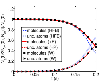
Figure 1: (Color online) Comparison of the fractional particle numbers for $t_{{\tiny\mathnormal{final}}}$ = 0.20 s, for the case of a non-uniform condensate with $U_{1D}=0$, for positive-$P$ (red solid and dashed lines), truncated Wigner (black $\blacksquare$ and $\blacktriangleright$) and HFB (blue dashed lines) methods. The fractional atom numbers (initially lower curves) and the fractional molecule numbers are shown. In this figure and throughout this paper, the positive-$P$ and truncated Wigner results are for the case of 10,000 trajectories. The error bars are shown and are essentially the thickness of the data lines in all figures. In all simulations performed the initial number of molecules is $N_{m}(0)=1.62\times 10^{3}$.

The positive-$P$ method becomes intractable at $t\sim 0.20$ s, and hence the ability to compare all three methods ceases beyond this point. Looking forward, when one incorporates $s$-wave scattering the positive-$P$ method will fail sooner Savage et al. (2006) and hence the truncated Wigner and HFB methods may be able to access a regime otherwise inaccessible to numerical simulations for realistic non-uniform condensates.

V.3 Observation of Phase Diffusion Processes During Dissociation of a Molecular BEC

In this section we consider non-uniform condensates with $s$-wave scattering interactions included. In Fig. 2, we plot the fractional particle number throughout the evolution, for the same parameters as in Fig. 1, but with scattering included. We choose an interaction strength of $U_{1D}\equiv g_{0}=1.04\times 10^{-6}\omega_{\perp}a_{s}$, which corresponds to ⁸⁷Rb with transverse confinement of $\omega_{\bot}/2\pi=30$ Hz and s-wave scattering length of $a_{s}=5.4$ nm. From these results it can be seen that the positive-$P$ method fails beyond approximately $t_{\max}(+\mathnormal{P})=0.18$ s, whilst the truncated Wigner method produces results beyond $t_{\max}(+P)$ and still does well in comparison to the positive-$P$ results up to $t_{\max}(+P)$. As expected Savage et al. (2006), we find that the positive-$P$ method fails for even shorter times as the interaction strength is increased. For example, with an interaction strength of $U_{1D}=32g_{0}$ we find that the positive-$P$ method fails for $t_{\max}(+\mathnormal{P})\sim 0.05$ s.

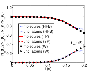
Figure 2: (Color online) As in Fig. 1, except for the case of a non-uniform condensate with $U_{1D}=g_{0}$. The positive-$P$ method becomes intractable beyond $t_{{\mathnormal{\tiny max}}}$(+P) $\sim 0.18$ s, compared with $t\sim 0.2$ s when $s$ -wave scattering is neglected. We also find that the number of molecules converted into atom pairs is decreased when $s$-wave scattering interactions are included and attribute this to phase diffusion.

Here we also observe the signature of phase diffusion during molecular dissociation Lewenstein and You (1996); Steel et al. (1998); Xiong et al. (2002); Li et al. (2001). By considering Eq. (5) we are able to estimate the characteristic diffusion time for the dissociation process,

$$t_{d}\sim\frac{\pi}{2U_{1D}\langle\hat{\Psi}^{\dagger}(x=0,t_{d})\hat{\Psi}(x=0,t_{d})\rangle},$$ (12)

and verify that the process of phase diffusion is responsible for suppressing molecular conversion, and hence, decreasing the number of atom pairs formed. We also performed simulations for increased values of the atom-atom interaction strength, $U_{1D}=2g_{0}$ and $U_{1D}=32g_{0}$. The results show that molecule conversion decreases with increasing interaction strength and further supported the order of magnitude estimates of the diffusion time. Unfortunately, as in Sec. V.2, we see that the HFB method still fails to adequately describe the dynamics of the molecular dissociation process for longer times, with the particle numbers only providing bounds for the true values. Another feature indicative of the limitations of the HFB method is its inability to predict the formation of peaks in the molecular momentum spectrum at $\pm 2k_{0}$ mag , in addition to the main resonant momenta peaks formed at $\pm k_{0}$. These secondary peaks arise due to atom-atom recombination processes $k_{0}+k_{0}\rightarrow 2k_{0}$ and $-k_{0}-k_{0}\rightarrow-2k_{0}$, and are observed in the positive-$P$ and truncated Wigner results. They do not arise in the HFB results as the method does not allow for uncondensed molecules outside the initial condensate mode.

V.4 Analysis of Atomic Pair-Correlation Functions

We have also investigated atomic pair-correlations resulting from the dissociation process, for realistic non-uniform condensates including the effects of $s$-wave scattering. The strength of atom-atom correlations can be quantified using Glauber’s second-order correlation function $g^{(2)}(\mathbf{k},\mathbf{k}^{\prime},t)$ Glauber (1963),

$$g^{(2)}(\mathbf{k},\mathbf{k}^{\prime},t)=\frac{\left\langle\hat{a}^{\dagger}(\mathbf{k},t)\hat{a}^{\dagger}(\mathbf{k}^{\prime},t)\hat{a}(\mathbf{k}^{\prime},t)\hat{a}(\mathbf{k},t)\right\rangle}{\left\langle\hat{n}(\mathbf{k},t)\right\rangle\left\langle\hat{n}(\mathbf{k}^{\prime},t)\right\rangle},$$ (13)

with the momentum-space density at $\mathbf{k}$ given by $n(\mathbf{k},t)=\left\langle\hat{n}(\mathbf{k},t)\right\rangle=\left\langle\hat{a}^{\dagger}(\mathbf{k},t)\hat{a}(\mathbf{k},t)\right\rangle$ where the momentum-space field amplitudes are represented by the lattice-discretized momentum components $\hat{a}^{\dagger}(\mathbf{k})$ and $\hat{a}(\mathbf{k})$, which correspond to the continuous Fourier transforms of the fields in the limit $\Delta k\rightarrow 0$ Savage et al. (2006). This pair-correlation function describes the ratio of the probability of the joint detection of atom pairs with $\mathbf{k}$ and $\mathbf{{k}^{\prime}}$ to the product of the probabilities of independent atom detection at $\mathbf{k}$ and $\mathbf{{k}^{\prime}.}$ From this it follows that $g^{(2)}(\mathbf{k},\mathbf{k}^{\prime},t)=1$ for uncorrelated atom pairs, $g^{(2)}(\mathbf{k},\mathbf{k}^{\prime},t)=2$ for thermally bunched atoms and $g^{(2)}(\mathbf{k},\mathbf{k}^{\prime},t)>2$ for strongly correlated atoms Savage et al. (2006).

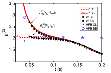
Figure 3: (Color online) Plot of the atomic pair-correlation functions for back-to-back and collinear scattering processes, denoted $g^{(2)}_{BB}(k_{0},-k_{0},t)$ and $g^{(2)}_{CL}(k_{0},k_{0},t)$. Results are shown for $t_{\mathnormal{\tiny final}}$ = 0.20 s, for a non-uniform condensate with $U_{1D}=0$. The positive-$P$ results (red solid and dashed lines), the truncated Wigner results (black $\blacksquare$ and $\blacktriangleright$) and the HFB results (blue $\circ$ and $\ast$) are shown. The collinear (red dashed, black $\blacktriangleright$ and blue $\ast$) and the back-to-back pair-correlations (red solid, black $\blacksquare$ and blue $\circ$) are shown.

We quantify pair-correlations arising due to momentum conservation which are present between atoms with equal but opposite momenta, and pair-correlations arising due to quantum statistical effects [i.e. the Hanbury-Brown and Twiss (HBT) bunching] between atoms scattered in the same direction. The atomic pair-correlations function for back-to-back (BB) and collinear (CL) scattering processes, are denoted $g_{BB}^{(2)}(k_{0},-k_{0},t)$ and $g_{CL}^{(2)}(k_{0},k_{0},t)$, respectively. These quantities are shown in Fig. 3 for the case of no $s$-wave scattering and in Fig. 4 with scattering incorporated. The collinear correlation indicates HBT thermal bunching with $g_{CL}^{(2)}(k_{0},k_{0},t)=2$ until $t\sim 0.10$ s in both cases. The back-to-back correlation is super-bunched due to strong correlations between atom pairs with equal but opposite momenta, with $g_{BB}^{(2)}(k_{0},-k_{0},t)>2$ for short times. Beyond $t\sim 0.10$ s we observe both the collinear and back-to-back correlations are approximately equal, fall below two, and approach the uncorrelated or coherent level of $g^{(2)}=1$, for the truncated Wigner and positive-$P$ results. The HFB results, on the other hand, fail to predict where $g^{(2)}$ approaches the coherent state level as stimulated processes become important. Toward the end of the simulation, the back-to-back correlation drops below the collinear correlation, $g_{BB}^{(2)}(k_{0},-k_{0},t)<g_{CL}^{(2)}(k_{0},k_{0},t)$. This effect becomes more severe with increasing values of $U_{1D}$ and is also noticeable in the HFB results.

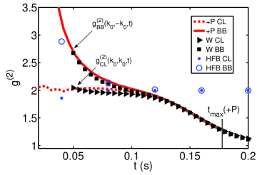
Figure 4: (Color online) As in Fig. 3, except for the case of a non-uniform condensate with $U_{1D}=g_{0}$. The positive-$P$ method becomes intractable beyond $t_{{\mathnormal{\tiny max}}}$(+P)$\sim 0.18$ s, compared with $t\sim 0.2$ s when $s$ -wave scattering is neglected. By comparison with Fig. 3, we see that the back-to-back and collinear pair-correlation strength degrades at an increased rate when $s$-wave scattering is included.

From Figs. 3 and 4 it is again clear that the truncated Wigner method is most successful in describing molecular dissociation, with the positive-$P$ method intractable at longer times. It should be noted that the truncated Wigner results for this correlation function are not shown prior to $t\sim 0.05$ s, where sampling issues arise due to the small number of atoms per mode. However, once the signal is significant the results agree with positive-$P$. As seen in Sec. V B and C, the HFB method fails to fully describe the dynamics for longer times as the molecular field deviates from the assumed coherent state.

VI Simulations beyond $t_{\max}(+P)$

The numerical results we have presented indicate that the HFB method is unsuitable for quantitative correlation studies of molecular dissociation beyond the regime of the positive-$P$ simulations. The HFB method becomes invalid as it assumes a mean-field coherent state for molecules for the entire simulation time Jack and Pu (2005); Davis et al. (2008). However, once molecular depletion reaches $\sim 80\%$, this assumption is no longer valid and the method becomes increasingly inadequate as the regime of complete depletion is reached. This assertion is further supported in Fig. 5, which provides a surface plot of the molecular density in position space beyond $t_{\max}(+P)$. Here we begin to observe the development of ripple effects which coincide with the reduction of the molecular condensate density and it is unlikely that the approximation of the molecular field as a coherent state is still valid. In this regime the effects of quantum fluctuations become increasingly important and hence, we cannot rely on the HFB method. To remedy this, the inclusion of molecular fluctuations $\hat{\chi}_{m}$ in the HFB formalism could be one avenue for future work. It should be stressed that there is value in using the HFB method, as it lies between the crude undepleted, molecular field approximation and an exact quantum treatment. For instance, the HFB approach is suited to high energy, sparsely occupied modes Bezett et al. (2008). In such cases, fluctuation effects are largely insignificant and the HFB method is valuable.

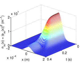
Figure 5: (Color online) Molecular density in position space $n_{m}(x)$ [in units of m^-1] as a function of time for the HFB results. The molecular peak density is given by $n_{0}=1.83\times 10^{7}$m^-1.

With the HFB approach found to be invalid beyond the realm of the positive-$P$ simulations, we look at extending the simulations using the truncated Wigner approach. Fig. 6 and 7 repeat the analysis given in Sec. V but with the extension to $t=0.40$ s. In Fig. 6 we again look at the fractional particle numbers for the cases neglecting and including atom-atom interactions. Beyond $t\sim 0.2$ s, for the $U_{1D}=0$ case we observe the effects of atom-atom recombination. This is apparent due to the slight increase in the number of molecules, and corresponding decrease in the number of atoms, until $t\sim 0.3$ s. With the effects of $s$-wave scattering included, we again witness a phase diffusion process which is responsible for decreasing the rate of molecule conversion.

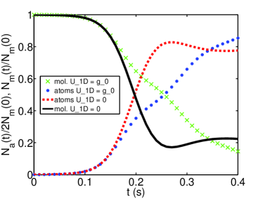
Figure 6: (Color online) Fractional particle numbers for $t_{{\tiny\mathnormal{final}}}$ = 0.40 s, for the case of a non-uniform condensate with $U_{1D}=0$ (black solid line and red dashed line) and $U_{1D}=g_{0}$ (green crosses and blue dotted), for the truncated Wigner results. The fractional atom number (blue dotted and red dashed) and the fractional molecule number (black solid and green crosses) are shown. For the $U_{1D}=0$ case for $t>$ 0.20 s, we observe an increase in the molecular population from atom-atom recombination. With the inclusion of $s$-wave scattering interactions we again see the effects of phase diffusion.

In Fig. 7 we provide the truncated Wigner results for the back-to-back and collinear pair-correlation functions for the cases where $s$-wave scattering interactions are neglected and included. In both cases, the back-to-back correlation is exceeded by the collinear correlation, i.e. $g_{BB}^{(2)}(k_{0},-k_{0},t)<g_{CL}^{(2)}(k_{0},k_{0},t)$, with the effect becoming more dramatic with time. It is interesting to note that when atom-atom interactions are neglected the back-to-back pair correlation eventually turns into anti-correlation, ie. $g^{(2)}_{BB}(k_{0},-k_{0})<1$, for sufficiently long times when the molecular depletion is large. As the atomic density increases, we see atom-atom recombination which is not correlated at the two momenta considered, so that atoms are not removed equally from each of the modes under consideration. Overall, by using the truncated Wigner method to go beyond the realm of the positive-$P$ simulations, we are able to observe the effects of $s$-wave scattering on correlation dynamics for realistic inhomogeneous condensates.

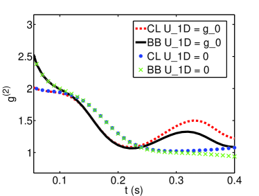
Figure 7: (Color online) Plot of the atomic pair-correlation functions for back-to-back (black solid and green crosses) and collinear (blue dotted and red dashed) scattering processes, $g^{(2)}_{BB}(k_{0},-k_{0},t)$ and $g^{(2)}_{CL}(k_{0},k_{0},t)$, respectively. Results are shown for $t_{\mathnormal{\tiny final}}=0.40$ s, for a non-uniform condensate with $U_{1D}=0$ (blue dotted and green crosses) and $U_{1D}=g_{0}$ (black solid and red dashed). The back-to-back correlation drops below the collinear correlation.

VII Conclusions

In this work we have compared three different theoretical approaches to the problem of dissociation of molecular Bose-Einstein condensates. We have considered the case where the atoms resulting from this dissociation process are not trapped, but move away from the parent molecules with momenta that are a function of the detuning. In particular, we have calculated atomic and molecular populations and analysed the effects of atom-atom interactions beyond the short time limit for inhomogeneous condensates. We have also investigated quantum correlations, providing quantitative results for the back-to-back and collinear pair-correlations, which cannot be calculated in the standard mean-field Gross-Pitaevskii approach. This is a subject of immediate interest as experiments which can measure these correlations can now be performed, particularly with metastable helium Perrin et al. (2007).

In principle, the preferred theoretical method would be the stochastic integration of equations in the positive-$P$ representation, as these give complete access to all properties of the interacting many-body quantum system. In practice, however, the problems inherent in the integration of these equations, especially when $s$-wave interactions of any appreciable strength are present, mean that the positive-$P$ equations are only useful for short times. Another method which has been widely applied to model BEC dynamics is the HFB approach. In some sense this is equal to the commonly used linearisation procedures of quantum optics, and similarly to that area, we find that we must be careful with its validity. In fact, we have shown here that the HFB approach will sometimes become inaccurate on shorter time scales than those which give problems in the positive-$P$ representation approach. Although it does present computational advantages in that the equations need only be solved once by contrast with the phase-space representations where averages need to be taken over many realisations, we see that it is also not useful for all parameter regimes. This could be remedied, at least in part, by including the effects of molecular fluctuations. However, this is a cumbersome and computationally expensive process.

We have found that the most useful of the methods is the truncated Wigner representation. Although the approximations necessary to obtain stochastic differential equations mean that the mapping from the quantum Hamiltonian is not exact, we find that the truncated Wigner method agrees with the first-principle positive-${P}$ results whenever such a comparison is possible to make. It also has the advantages of not suffering from the stability problems of the positive-$P$ representation and is valid over longer times than the HFB approach. In conclusion therefore, we find that while the positive-$P$ and HFB approaches are useful in some regimes, the truncated Wigner representation is best suited to this problem.

References

- Thompson et al. (2005) S. T. Thompson, E. Hodby, and C. E. Wieman, Phy. Rev. Lett. 94, 020401 (2005).
- Greiner et al. (2005) M. Greiner et al., Phys. Rev. Lett. 94, 110401 (2005).
- Drr et al. (2004) S. Drr, T. Volz, and G. Rempe, Phys. Rev. A 70, 031601 (2004).
- Mukaiyama et al. (2004) T. Mukaiyama et al., Phys. Rev. Lett. 92, 180402 (2004).
- Kheruntsyan et al. (2005) K. V. Kheruntsyan, M. K. Olsen, and P. D. Drummond, Phys. Rev. Lett. 95, 150405 (2005).
- Savage and Kheruntsyan (2007) C. M. Savage and K. V. Kheruntsyan, Phys. Rev. Lett. 99, 220404 (2007).
- Opatrny and Kurizki (2001) T. Opatrny and G. Kurizki, Phys. Rev. Lett. 86, 3180 (2001).
- Perrin et al. (2007) A. Perrin et al., Phy. Rev. Lett. 99, 150405 (2007).
- Flling et al. (2005) S. Flling et al., Nature 434, 481 (2005).
- Altman et al. (2004) E. Altman, E. Demler, and M. D. Lukin, Phys. Rev. A 70, 013603 (2004).
- Bach and Rza̧żewski (2004) R. Bach and K. Rza̧żewski, Phys. Rev. Lett. 92, 200401 (2004).
- Schellekens et al. (2005) M. Schellekens et al., Science 310, 648 (2005).
- (13) F. Lang et al., arXiv:0809.0061.
- Savage et al. (2006) C. M. Savage, P. E. Schwenn, and K. V. Kheruntsyan, Phys. Rev. A 74, 033620 (2006).
- Kheruntsyan (2006) K. V. Kheruntsyan, Phys. Rev. Lett. 96, 110401 (2006).
- Kheruntsyan (2005) K. V. Kheruntsyan, Phys. Rev. A 71, 053609 (2005).
- Kheruntsyan and Drummond (2002) K. V. Kheruntsyan and P. D. Drummond, Phys. Rev. A 66, 031602 (2002).
- Poulsen and Mølmer (2001) U. V. Poulsen and K. Mølmer, Phys. Rev. A 63, 023604 (2001).
- Jack and Pu (2005) M. W. Jack and H. Pu, Phys. Rev. A 72, 063625 (2005).
- Zhao et al. (2007) B. Zhao et al., Phy. Rev. A. 75, 042312 (2007).
- Moore and Vardi (2002) M. G. Moore and A. Vardi, Phy. Rev. Lett. 88, 160402 (2002).
- Tikhonenkov and Vardi (2007) I. Tikhonenkov and A. Vardi, Phy. Rev. Lett. 98, 080403 (2007).
- Anderson et al. (1995) M. H. Anderson et al., Science 269 (1995).
- Pethick and Smith (2002) C. Pethick and H. Smith, Bose-Einstein Condensation in Dilute Gases (Cambridge University Press, United Kingdom, 2002).
- Holland et al. (2001) M. Holland, J. Park, and R. Walser, Phys. Rev. Lett. 86, 1915 (2001).
- Drummond and Corney (1999) P. D. Drummond and J. F. Corney, Phys. Rev. A 60, R2661 (1999).
- Hope and Olsen (2001) J. J. Hope and M. K. Olsen, Phys. Rev. Lett. 86, 3220 (2001).
- gren and Kheruntsyan (2008) M. gren and K. V. Kheruntsyan, Phys. Rev. A 78, 011602(R) (2008).
- Davis et al. (2008) M. J. Davis et al., Phys. Rev. A 77, 023617 (2008).
- Drummond and Gardiner (1980) P. D. Drummond and C. W. Gardiner, J. Phys. A 13, 2353 (1980).
- Drummond and Carter (1987) P. D. Drummond and S. J. Carter, J. Opt. Soc. Am. B 4, 1565 (1987).
- Steel et al. (1998) M. J. Steel et al., Phys. Rev. A 58, 4824 (1998).
- Sinatra et al. (2001) A. Sinatra, C. Lobo, and Y. Castin, Phys. Rev. Lett. 87, 210404 (2001).
- Milstein et al. (2003) J. N. Milstein, C. Menotti, and M. Holland, New Journal of Physics 5, 52.1 (2003).
- Morgan (2005) S. A. Morgan, Phys. Rev. A 72, 043609 (2005).
- Hutchinson et al. (1998) D. A. W. Hutchinson, R. J. Dodd, and K. Burnett, Phys. Rev. Lett. 81, 2198 (1998).
- Griffin (1996) A. Griffin, Phys. Rev. B 53, 9341 (1996).
- Heinzen et al. (2000) D. J. Heinzen et al., Phys. Rev. Lett. 84, 5029 (2000).
- Deuar and Drummond (2007a) P. Deuar and P. D. Drummond, Phys. Rev. Lett. 98, 120402 (2007a).
- Deuar and Drummond (2006a) P. Deuar and P. D. Drummond, J. Phys. A 39, 2723 (2006a).
- Gilchrist et al. (1997) A. Gilchrist, C. W. Gardiner, and P. D. Drummond, Phys. Rev. A 55, 3014 (1997).
- Timmermans et al. (1999) E. Timmermans et al., Phys. Rep. 315, 199 (1999).
- Duine and Stoof (2004) R. A. Duine and H. T. C. Stoof, Phys. Rep. 86, 115 (2004).
- Khler et al. (2006) T. Khler, K. Góral, and P. S. Julienne, Rev. Mod. Phys. 78, 1311 (2006).
- Drummond and Kheruntsyan (2004) P. D. Drummond and K. V. Kheruntsyan, Phy. Rev. A. 70, 033609 (2004).
- Norrie et al. (2006) A. A. Norrie, R. J. Ballagh, and C. W. Gardiner, Phys. Rev. A 73, 043617 (2006).
- Lobo et al. (2004) C. Lobo, A. Sinatra, and Y. Castin, Phy. Rev. Lett. 92, 020403 (2004).
- Gardiner and Zoller (2000) C. W. Gardiner and P. Zoller, Quantum Noise, 2nd Ed. (Springer, 2000).
- Deuar and Drummond (2006b) P. Deuar and P. D. Drummond, J. Phys. A: Math Gen. 39, 1163 (2006b).
- Deuar and Drummond (2006c) P. Deuar and P. D. Drummond, J. Phys. A: Math Gen. 39, 2723 (2006c).
- Corney and Drummond (2003) J. F. Corney and P. D. Drummond, Phys. Rev. A 68, 068322 (2003).
- Olsen and Plimak (2003) M. K. Olsen and L. I. Plimak, Phys. Rev. A 68, 031603 (2003).
- Olsen (2004) M. K. Olsen, Phys. Rev. A 69, 013601 (2004).
- Olsen et al. (2004) M. K. Olsen, A. S. Bradley, and S. B. Cavalcanti, Phys. Rev. A 70, 033611 (2004).
- Walls and Milburn (1995) D. F. Walls and G. J. Milburn, Quantum Optics, 2nd Ed. (Springer, 1995).
- Plimak et al. (2001) L. Plimak, M. K. Olsen, M. Fleischhauer, and M. J. Collett, Europhys. Lett. 56 (2001).
- Olsen et al. (2001) M. K. Olsen, K. Dechoum, and L. I. Plimak, Opt. Commun. 190 (2001).
- Sinatra et al. (2002) A. Sinatra, C. Lobo, and Y. Castin, J. of Phys. B 35, 3599 (2002).
- Bach et al. (2002) R. Bach, M. Trippenbach, and K. Rza̧żewski, Phys. Rev. A 65, 063605 (2002).
- Zin et al. (2005) P. Zin et al., Phys. Rev. Lett. 94, 200401 (2005).
- Javanainen et al. (2002) J. Javanainen et al., Phys. Rev. Lett. 92, 200402 (2002).
- Wster et al. (2005) S. Wster, J. Hope, and C. M. Savage, Phys. Rev. A 71, 033604 (2005).
- Blaizot and Ripka (1986) J. P. Blaizot and G. Ripka, Quantum theory of finite systems (MIT Press, Cambridge, MA, 1986).
- Reid and Drummond (1989) M. D. Reid and P. D. Drummond, Phys. Rev. A 40, 4493 (1989).
- Deuar and Drummond (2007b) P. Deuar and P. D. Drummond, Phy. Rev. Lett. 98, 0120402 (2007b).
- Kheruntsyan et al. (2005) K. V. Kheruntsyan et al., Phys. Rev. A 71, 053615 (2005).
- (67) XMDS documentation available at www.xmds.org.
- Lewenstein and You (1996) M. Lewenstein and L. You, Phys. Rev. Lett. 77, 3489 (1996).
- Xiong et al. (2002) H. Xiong, S. Liu, and G. Huang, Phys. Lett. A 301, 203 (2002).
- Li et al. (2001) W. Li et al., Phys. Lett. A 285, 45 (2001).
- (71) M. Ögren, private communication.
- Glauber (1963) R. Glauber, Phys. Rev. A 130, 2529 (1963).
- Bezett et al. (2008) A. Bezett, E. Toth, and P. B. Blakie, Phys. Rev. A 77, 023602 (2008).