NMR Response in quasi one-dimensional Spin-$\frac{1}{2}$ Antiferromagnets

Abstract

Non-magnetic impurities break a quantum spin chain into finite segments and induce Friedel-like oscillations in the local susceptibility near the edges. The signature of these oscillations has been observed in Knight shift experiments on the high-temperature superconductor YBa₂Cu₃O_6.5 and on the spin-chain compound Sr₂CuO₃. Here we analytically calculate NMR spectra, compare with the available experimental data for Sr₂CuO₃, and show that the interchain coupling is responsible for the complicated and so far unexplained lineshape. Our results are based on a parameter-free formula for the local susceptibility of a finite spin chain obtained by bosonization which is checked by comparing with quantum Monte Carlo and density-matrix renormalization group calculations.

1 Introduction

An important tool to study the local spin dynamics in strongly correlated electron systems is nuclear magnetic resonance (NMR). NMR experiments have been instrumental in investigating spin fluctuations and impurity effects in high-temperature superconductors [1], as well as in confirming the triplet nature of superconductivity in Sr₂RuO₄ [2]. Quite recently, NMR was also used to study the CuO chains in YBa₂Cu₃O_6.5 (YBCO) [3]. The NMR study showed that the chain ends induce Friedel-like oscillations which manifest themselves also in the CuO₂ planes. Similar oscillations have also been observed earlier in the prototypical quasi one-dimensional $S=1/2$ spin chain compound Sr₂CuO₃ (SCO) [4, 5]. Theoretically, a large alternating component of the local susceptibility near the end of a semi-infinite Heisenberg chain has been predicted [6]. Other studies (for a recent review see ref. [7]) have addressed local spin correlations near a chain end by numerical means in a variety of one-dimensional models ranging from the frustrated and dimerized spin-$1/2$ chain to spin ladders and the spin-$1$ Heisenberg chain [8].

An interesting open question concerning the physics of the spin-$1/2$ Heisenberg chain is whether its transport properties are ballistic or diffusive. The theoretical results are contradictory [9, 10, 11, 12, 13, 14] but seem to point to ballistic transport perhaps related to the integrability of the model by Bethe ansatz. NMR and muon spin relaxation experiments on SCO [15, 16], on the other hand, have found diffusive behavior. In order to analyze these experiments on a quantitative level in the future, it is first of all important to know in how far a spin-only model for SCO is valid. In particular, it has been claimed in ref. [5] that already the NMR spectra - where only static correlations are tested - can only be understood if a coupling to the lattice is taken into account.

In the first part of this letter we will calculate NMR spectra for a Heisenberg chain with a Poisson distribution of non-magnetic impurities.This is known to be the relevant model for SCO, with chain breaks caused by the presence of excess oxygen [17, 18]. We will start with the ideal chain but will then show that the interchain couplings are essential to fully explain the experimental data for SCO [4, 5]. Our main findings are that the theoretically calculated spectra for a spin-only model of weakly coupled Heisenberg chains are in perfect agreement with experiment whereas the phenomenological model proposed in [5], involving some coupling to lattice degrees of freedom, cannot - if taken seriously - explain the data. The calculated NMR spectra are based on a parameter-free formula for the local susceptibility of finite $S=1/2$ $XXZ$ chains at finite temperatures obtained by a bosonization approach as explained in the second part of this letter. The analytical results allow for a full impurity averaging which would be impossible to achieve at low temperatures by numerical calculations.

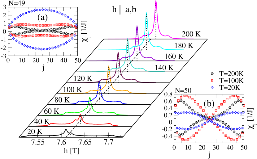
Figure 1: (Color online) Theoretical NMR spectra (3) for a Poisson distribution with $p=0.3\%$ non-magnetic impurities, parameters $J,\,A^{0},\,A^{\pm 1}$ as appropriate for SCO (see text), $\Gamma=4\cdot 10^{-4}$, and $h_{\rm res}^{0}=7.61$ T (dashed line). The dotted lines mark the maxima corresponding to the bulk susceptibility. Insets (a) and (b) show local susceptibilities at various temperatures indicated on the plot.

2 NMR spectra

The Hamiltonian of the spin-$1/2$ $XXZ$ model with $N$ sites and open boundary conditions (OBCs) is given by

$$H=J\sum_{j=1}^{N-1}\left[S^{x}_{j}S^{x}_{j+1}+S^{y}_{j}S^{y}_{j+1}+\Delta S^{z}_{j}S^{z}_{j+1}\right]-h\sum_{j=1}^{N}S^{z}_{j}\;.$$ (1)

Here $J$ is the exchange constant, $\Delta\in[0,1]$ an exchange anisotropy, and $h$ the applied magnetic field. Due to the OBCs, translational invariance is broken leading to a position dependent local susceptibility

$$\chi^{(N)}_{j}=\frac{\partial}{\partial h}\langle S^{z}_{j}\rangle_{h=0}=\frac{1}{T}\langle S^{z}_{j}S^{z}_{\rm tot}\rangle_{h=0}$$ (2)

where $T$ is the temperature and $S^{z}_{\rm tot}=\sum_{j}S^{z}_{j}$. The hyperfine interaction couples nuclear and electron spins. For a chain segment of length $N$ this leads to the Knight shift of the nuclear resonance frequency $K^{(N)}_{j}=(\gamma_{e}/\gamma_{n})\sum_{j^{\prime}}A^{j-j^{\prime}}\chi^{(N)}_{j^{\prime}}$, where $\gamma_{e}$ ($\gamma_{n}$) is the electron (nuclear) gyromagnetic ratio, respectively. The hyperfine interaction is short ranged so that usually only $A^{0}$ and $A^{\pm 1}$ matter. The NMR spectrum is proportional to the distribution of Knight shifts. Let us assume in the following a Poisson distribution of non-magnetic impurities with concentration $p$ and a Lorentzian lineshape with width $\Gamma$ for each Knight shift. The normalized probability distribution is then given by

$$P(K)=\frac{\Gamma}{\pi}\!\!\sum_{N=1}^{\infty}\frac{p(1-p)^{N-1}}{N}\!\sum_{j=1}^{N}\frac{1}{(K-K^{(N)}_{j})^{2}+\Gamma^{2}}\;.$$ (3)

As we will show in the second part of this letter, bosonization allows us to derive a parameter-free result for $\chi_{j}^{(N)}$ in the limit $T/J\ll 1$ and $N\gg 1$. Because the deviations for very small chain lengths are not important for the NMR spectra as long as the probability of having such tiny segments is low, the only parameters entering in (3) are the material-dependent constants $J$, $A^{0}$ and $A^{\pm 1}$.

NMR measurements have been performed on the Heisenberg ($\Delta=1$) chain compound SCO [4, 5]. Chain breaks in this system are believed to be caused by randomly distributed excess oxygen leading to the formation of Zhang-Rice singlets [17, 18]. From measurements of the total susceptibility it follows that $J\sim 2200$ K [17]. By a comparison with YBa₂Cu₃O_6+δ [19] and theory the hyperfine coupling constants $A_{c}^{0}/(2\hbar\gamma_{n})\approx-13$ T, $A_{ab}^{0}/(2\hbar\gamma_{n})\approx 2$ T, and $A^{1}/(2\hbar\gamma_{n})\approx 4$ T are obtained. Here the index denotes the magnetic field direction. We calculate the spectra as a function of $h=(1+K)h_{\rm res}^{0}$ where $h_{\rm res}^{0}=\nu/\gamma_{n}$ is the resonance field for an isolated ⁶³Cu atom. In experiment $\nu=86$ MHz [4] and $\gamma_{n}\approx 11.3$ MHz/T [20] leading to $h_{\rm res}^{0}\approx 7.61$ T. Exemplarily, we show the evolution of the lineshape for an ideal chain with impurity concentration $p=0.3\%$ in fig. 1. At high temperatures a central peak dominates whose position corresponds to the bulk susceptibility value. In addition, broad edges are visible whose separation increases $\sim h^{0}_{\rm res}\sqrt{v/T}\ln^{1/4}(v/T)$ with decreasing temperature with $v$ being the spin velocity. These edges are caused by the extrema in the local susceptibilities of chain segments with lengths $N\gg\pi v/T$ (see Figs. 1 (a) and (b), respectively). Furthermore, we observe a gradual transfer of weight from a peak at high temperatures to a peak corresponding to zero Knight shift at low temperatures stemming from the increasing number of even chain segments with $N\ll\pi v/T$ which become frozen into their singlet ground state (see fig. 1(b)). The odd chain segments with $N\ll\pi v/T$, on the other hand, will yield large Knight shifts (see fig. 1(a)). This leads to a background which grows in intensity and expands with decreasing temperature. The temperature $T^{*}$ where the peak corresponding to zero Knight and the peak corresponding to the bulk susceptibility value have equal height is therefore directly related to the impurity concentration. For $p\ll 1$ we analytically find

$$p\approx 1-3^{-2T^{*}/(J\pi^{2})}$$ (4)

which is a simple criterion to determine the impurity concentration from the NMR spectra alone.

The observation of a central peak at high temperatures and broad edges with separation $\Delta h\sim h^{0}_{\rm res}\sqrt{v/T}$ is in agreement with experimental observations [4, 5] as shown in fig. 2. It has indeed already been pointed out in [4] - based on the theoretical results for the semi-infinite chain by Eggert and Affleck [6] - that the edges are a consequence of the maxima in the local susceptibility.

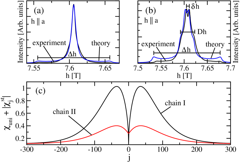
Figure 2: (Color online) (a) Comparison between experimental data taken from [4] and theory with material-dependent parameters as given in the text and $p=5\times 10^{-4}$, $\Gamma=4\times 10^{-4}$ at $T=60$ K. The peak height has been adjusted to agree with experiment and $h^{0}_{\rm res}=7.5955$. (b) Same as (a) at $T=30$ K. (c) Calculated oscillations $\chi_{j}$ at $T=30$ K in an infinite chain with an impurity at $x=0$ (chain I) and reflections in the infinite chain II without impurities due to an interchain coupling with strength $J_{\perp}=5$ K.

However, at temperatures $T\lesssim 30$ K additional structures are visible in the experimental spectra. The peak develops shoulders whose separation is denoted by $Dh$ in fig. 2(b) following the notation introduced in [4]. Furthermore, a splitting of the peak, $\delta h$, very different from the weight transfer with temperature shown in fig. 1, is observed. In ref. [5] it has been tried to explain these features by a phenomenological model of mobile bond defects. In particular, the feature $\delta h$ was ascribed to a periodic arrangement of bond defects leading to chain segments of odd length $N$ only. However, analytically we find that the splitting of the central peak would then grow like $\sim h^{0}_{\rm res}J\ln^{1/4}(N)/(TN^{1/2})$. Due to the prefactor $\sim J$ this predicts a very rapid increase of the splitting not observed in experiment showing that this model is incorrect. Instead, as we will show below, the additional features $Dh$ and $\delta h$ are a consequence of the interchain coupling. The interchain coupling along one of the crystal axes perpendicular to the chains is of order $J_{\perp}\sim 5$ K while it is three orders of magnitude smaller along the other direction [17, 21]. At $T\sim 30$ K we might therefore already expect significant effects of the interchain couplings which, however, can be included perturbatively. Doing so we find that the susceptibility oscillations near an impurity residing in one chain (zeroth order) lead to substantial reflections in the neighboring chain (first order) for parameters appropriate for SCO as shown in fig. 2(c). The ratio of the maximum in chain I to the maximum in chain II is $\sim\Delta h/(Dh)$, i.e., the shoulders of the peak, $Dh$, are caused by the maxima of the reflected oscillations. We find $Dh\sim h^{0}_{\rm res}J_{\perp}\sqrt{v}T^{-3/2}$ but logarithmic corrections can disguise this scaling as will become clear later on. The splitting of the central peak $\delta h$, see fig. 2(b), has a more complicated origin. First, there are also a reflections in next-nearest neighboring chains (second order). The maxima would then yield a splitting $\delta h\sim h^{0}_{\rm res}J_{\perp}^{2}\sqrt{v}T^{-5/2}$ (again ignoring logarithmic corrections). However, for impurity concentrations $p\sim 5\times 10^{-4}$ relevant for the experiments there is another effect which actually dominates: Including the first and second order reflections from neighboring chains, the chain of average length $\bar{N}\approx 1/p$ will not have any sites left which show bulk behavior. This means that at temperatures $T\lesssim 30$ K the probability for having Knight shifts corresponding to values close to the bulk susceptibility starts to decrease dramatically thus leading to a drop in intensity in $P(K)$. Therefore $\delta h$ denotes not a splitting of the central peak but rather a dip of intensity at the bulk susceptibility value. The oscillations, which now basically spread over the entire crystal, might get further stabilized by anisotropic exchange terms. This might also explain the small differences in the lineshape near the peak for $h\parallel a$ and $h\parallel c$ [4, 5]. A detailed analysis of these anisotropy effects is beyond the scope of this letter.

We also want to stress that having additional structures in the spectra due to interchain couplings is very different from a scenario where instead such structures occur due to a direct hyperfine interaction or a dipolar coupling of the nuclear spins with electron spins in adjacent chains. The latter case would lead to $Dh/\Delta h=\mbox{const.}$ ($\delta h/\Delta h=\mbox{const.}$) as a function of temperature if the shoulders (splitting) are caused by this mechanism, respectively. Only three (two) different temperatures are presented in [5] where the shoulders (splitting) are visible, respectively, making a detailed analysis impossible. However, we find that the data are consistent with $Dh/\Delta h\sim 1/T$ as expected if interchain coupling dominates but certainly not consistent with either $Dh/\Delta h=\mbox{const.}$ or $\delta h/\Delta h=\mbox{const.}$.

To calculate the NMR lineshapes for SCO at low temperatures, we have to deal with a two-dimensional array of weakly coupled chains. In general, this is a very complicated task requiring a two-dimensional impurity averaging. However, for small impurity concentrations significant simplifications are possible. At a given temperature, the oscillations extend over a characteristic length $\xi$. If $\bar{N}=1/p\gg\xi$ then the probability of having two impurities in neighboring chains so close to each other that the zeroth order oscillations in the chain and the reflections from neighboring chains overlap is small. We therefore assume that reflections in a chain of length $N$ only occur in regions where the chain shows bulk behavior. In a chain of length $N$, $2pN$ reflections from the nearest neighbor chains and $2pN$ reflections from nearest-neighbor chains will occur on average. If a chain segment is long enough, we consider the zeroth, first, and second order oscillations as independent entities. If the segment is too short, we reduce the extend of the first and second order oscillations mimicking the overlap. For the chain segments we then do the full impurity averaging (3). The theoretically calculated lineshapes we obtain this way are in excellent agreement with experiment as shown in fig. 2. For both temperatures we use the peak to adjust the intensity. For $T=60$ K we also used $p$ and $h^{0}_{\rm res}$ as parameters and find $p=5\times 10^{-4}$ and $h^{0}_{\rm res}=7.5955$ T. In fig. 2 (b) we use the same values. An even better agreement would be obtained here if we choose $h^{0}_{\rm res}=7.598$ T which is equivalent to a deviation of $0.03\%$ from our prediction for the evolution of the bulk susceptibility value. Furthermore, the intensity of the edges $\Delta h$ is overestimated. This is most likely a consequence of our assumption that the zeroth order oscillations do not overlap with the reflections. Configurations where such an overlap occur would wash out the maxima of the zeroth order oscillations. In addition, this might also point to some deviations from a Poisson distribution with short chains occurring less frequently than expected.

3 Local susceptibility

We now explain how the parameter-free results for $\chi_{j}^{(N)}$ have been obtained. In the low-energy limit, the spin operators can be expressed in terms of a boson $\Phi$ as

$$S^{z}_{j}\approx\sqrt{\frac{K_{L}}{2\pi}}\partial_{x}\Phi+c(-1)^{j}\cos\sqrt{2\pi K_{L}}\Phi\;.$$ (5)

Here $K_{L}$ is the Luttinger parameter and $c$ the amplitude of the alternating part. The integrability of model (1) by Bethe ansatz allows it to determine $K_{L}$ and $c$ exactly for all $\Delta$. Ignoring bulk and boundary irrelevant operators, the Hamiltonian (1) is equivalent to a free boson model

$$H\! = \!\frac{v}{2}\int_{0}^{L+a}\!\!\!\!\!\!\!\!dx\left[\Pi^{2}+(\partial_{x}\Phi)^{2}\right]-h\sqrt{\frac{K_{L}}{2\pi}}\!\int_{0}^{L+a}\!\!\!\!\!\!\!\!dx\,\partial_{x}\Phi$$ (6)

where $v$ is the spin velocity, $L=Na$, and $a$ the lattice constant. The bosonic fields obey the standard commutation rule $[\Phi(x),\Pi(x^{\prime})]=\text{i}\delta(x-x^{\prime})$ with $\Pi=v^{-1}\partial_{t}\Phi$. To calculate the local susceptibility (2) we use a mode expansion

$$\Phi(x=ja,t)=\sqrt{\frac{\pi}{8K_{L}}}+\sqrt{\frac{2\pi}{K_{L}}}S^{z}_{\rm tot}\frac{j}{N+1}$$

$$+ \sum_{n=1}^{\infty}\frac{\sin\left(\pi nj/(N+1)\right)}{\sqrt{\pi n}}\left(\text{e}^{-i\frac{\pi nvt}{L+a}}b_{n}+\text{e}^{i\frac{\pi nvt}{L+a}}b_{n}^{\dagger}\right)$$

which incorporates the OBCs. Here $b_{n}$ is a bosonic annihilation operator. Eq. (3) is a discrete version of the mode expansions used in [22, 18] with $x=ja$ becoming a continuous coordinate for $a\to 0$, $N\to\infty$ with $L=Na$ fixed. Using this mode expansion, the local observables respect the discrete lattice symmetry $j\to N+1-j$ corresponding to a reflection at the central bond (site) for $N$ even (odd), respectively. The sites $0$ and $N+1$ are added to model (1) and we demand that the spin density vanishes at these sites. Therefore the upper boundary for the integrals in (6) is $L+a$. The zero mode part (first line of eq. (3)) fulfills $\sum_{j}S^{z}_{j}\approx\sqrt{\frac{K_{L}}{2\pi}}\int_{0}^{L+a}\partial_{x}\Phi\equiv S^{z}_{\rm tot}$ and the oscillator part (second line of eq. (3)) vanishes for $j=0,\,N+1$ as required.

Using (5) in the formula for the local susceptibility (2), we find $\chi_{j}=\chi_{j}^{\rm uni}+(-1)^{j}\chi_{j}^{\rm st}$. The uniform part is independent of position, $\chi_{j}^{\rm uni}\equiv\chi^{\rm uni}=\langle(S^{z}_{\rm tot})^{2}\rangle/(TN)$ and we can therefore directly use the parameter-free result derived in [18].

Figure 3: (Color online) $\chi_{j}$ for $\Delta=0.3$ and $T/J=0.02$. Comparison between QMC and field theory for $N=100$ and $N=99$.

For the staggered part, on the other hand, we find $\chi_{j}^{\rm st}=\frac{c}{T}\langle\cos\sqrt{2\pi K_{L}}\Phi\rangle_{\rm osc}\langle\cos\sqrt{2\pi K_{L}}\Phi S^{z}_{\rm tot}\rangle_{\rm zm}$ where we have split the correlation function into an oscillator and a zero mode part according to (3). Using the cumulant theorem for bosonic modes $\langle\exp(\pm\text{i}\sqrt{2\pi K_{L}}\Phi)\rangle_{\rm osc}=\exp(-\pi K_{L}\langle\phi\phi\rangle_{\rm osc})$ we obtain, following [23, 18],

$$\langle\cos\sqrt{2\pi K_{L}}\Phi\rangle_{\rm osc}=\left(\frac{\pi}{N+1}\right)^{K_{L}/2}\!\!\!\!\!\!\frac{\eta^{3K_{L}/2}\left(\text{e}^{-\frac{\pi v}{TL}}\right)}{\theta_{1}^{K_{L}/2}\left(\frac{\pi j}{N+1},\text{e}^{-\frac{\pi v}{2TL}}\right)}\,.$$ (8)

Here $\eta(x)$ is the Dedekind eta-function and $\theta_{1}(u,q)$ the elliptic theta-function of the first kind. For the zero mode part we find

$$\langle\cos\sqrt{2\pi K_{L}}\Phi S^{z}_{\rm tot}\rangle_{\rm zm}$$

$$= -\frac{\sum_{m}m\sin[2\pi mj/(N+1)]\text{e}^{-\pi vm^{2}/(K_{L}LT)}}{\sum_{m}\text{e}^{-\pi vm^{2}/(K_{L}LT)}}$$

with $m$ running over all integers (half-integers) for $N$ even (odd), respectively. In the thermodynamic limit, $N\to\infty$, we can simplify our result and obtain

$$\chi_{j}^{\rm st}=\frac{cK_{L}}{v}\frac{x}{\left[\frac{v}{\pi T}\sinh\left(\frac{2\pi Tx}{v}\right)\right]^{K/2}}$$ (10)

with $x=ja$. This agrees for the isotropic Heisenberg case, $K_{L}=1$, with the result in [6]. The amplitude $c$ can be determined with the help of the Bethe ansatz along the lines of ref. [24]. This leads to $c=\sqrt{A_{z}/2}$ with $A_{z}$ as given in eq. (4.3) of [24]. Our result for the staggered part of the local susceptibility is therefore parameter free. This means that we can directly compare our analytical result for $\chi_{j}$ with quantum Monte Carlo (QMC) data. For an anisotropy $\Delta=0.3$, shown in fig. 3, the agreement is excellent.

Figure 4: (Color online) $\chi_{j}$ for $\Delta=1$ and $N=100$. Comparison between QMC (closed symbols) and field theory (open symbols) for $T/J=0.02,~{}0.05,~{}0.1$, as indicated on the plot.

Next, we come to the experimentally most relevant isotropic case, $\Delta=1$ ($K_{L}=1$). Umklapp scattering is then marginally irrelevant and the scaling dimensions of correlation functions have to be replaced by renormalization group improved versions. For $\chi_{j}$ the calculations are rather similar to those in ref. [25] for the longitudinal spin-spin correlation function. We find that we have to replace $1/K_{L}\to 1-g$ in (3) whereas $K_{L}\equiv 1$ in the oscillator part, eq. (8). The renormalization of $K_{L}$ for this part is incorporated into an effective amplitude $c\to(2\pi^{3}g)^{-1/4}$. The running coupling constant $g$ depends, in general, on the three length scales $x$, $L$, and $v/T$. At low enough energies the smallest scale will always dominate and $g$ is given by the solution of $1/g+\ln(g)/2=\ln\left\{C_{0}\min[x,L-x,v/T]\right\}$ where $C_{0}$ is a constant. In fig. 4 a comparison between this analytic result and QMC data is shown with $C_{0}=6$. We note that fitting the constant $C_{0}$ improves the results near the boundaries. For low temperatures and $x,L-x\gg 1$, however, the value of $C_{0}$ becomes irrelevant and our result for $\chi_{j}$ therefore again parameter-free. The agreement with QMC is not as good as for the anisotropic case. This is a consequence of the fact that $g$ has been derived in the limit $x,L,v/T\gg 1$. However, the deviations are only of the order of a few percent and have very little effect on the NMR spectra presented in the first part of this letter.

Finally, the first order reflection $\chi_{j}^{\rm st(1)}$ of susceptibility oscillations in a neighboring chain, shown in fig. 2(c), is given in first order perturbation theory in $J_{\perp}$ by

$$\chi_{j}^{\rm st(1)}=-\frac{J_{\perp}}{T}(-1)^{j}\sum_{k}\chi_{k}^{\rm st}G^{zz,st}_{j-k}\,.$$ (11)

Here eq. (10) has to be used for $\chi_{k}^{\rm st}$ and $G^{zz,st}_{j-k}=\langle S^{z}_{j}S^{z}_{k}\rangle^{\rm st}=c^{2}/\left[\frac{v}{\pi T}\sinh(\frac{\pi T}{v}|j-k|)\right]^{K}$ is the staggered part of the bulk two-point correlation function. While it would be extremely difficult to obtain accurate numerical data for two weakly coupled chains at temperatures $T/J\sim 0.01$ as considered in fig. 2(c) we can easily check formula (11) at higher temperatures but still $T/J\ll 1$. Particularly suited to study the case of an infinite chain with a single non-magnetic impurity at the origin which is weakly coupled to an infinite chain without impurities is the density-matrix renormalization group (DMRG) applied to transfer matrices. This algorithm allows it to directly obtain results in the thermodynamic limit [26, 27]. In fig. 5, DMRG data are compared to the field theoretical formulas (10,11) and good agreement is found.

Figure 5: (Color online) $\chi_{j}^{\rm st}$ for $\Delta=1$, $J_{\perp}=0.03J$, and $T=0.1J$. Comparison between DMRG data (closed symbols) and field theory (open symbols) for an infinite chain with a non-magnetic impurity at $j=0$ (squares) and an infinite neighboring chain without impurities (circles).

The maximum of $|\chi_{j}^{\rm st(1)}|$ and therefore the separation of the shoulders $Dh$ scales like $T^{-3/2}$ for $K_{L}=1$ with complicated logarithmic corrections coming in through the amplitude $c$. This might make it hard to detect this power law in experiment. The second order reflections can be calculated analogously.

4 Conclusions

To conclude, we have derived an analytic formula for the local susceptibility of a finite Heisenberg chain. This allows us to calculate NMR spectra for spin chains with arbitrary impurity concentrations and distributions which would be impossible by numerical calculations at temperatures $T/J\ll 1$. We also showed how to calculate NMR spectra for weakly coupled spin chains if the impurities are dilute. For SCO we have demonstrated excellent agreement between our theory and experiment showing that SCO is indeed a prototypical quasi one-dimensional spin chain compound. More generally speaking, we have shown that NMR spectra are extremely useful to extract information about the impurity concentration as well as about the magnetic couplings. In particular, the coupling between the chains leads to an additional structure and its position allows it to directly extract the coupling strength. We also want to remark that this structure is very sensitive to the type of interchain coupling. If two chains are coupled by a zigzag-interchain coupling, as is the case, for example, for SrCuO₂ [17], $\chi_{j}^{\rm st(1)}$ would be zero, i.e., there would not be any reflections to first order in neighboring chains. An analysis of NMR spectra can therefore also help to clarify the geometry of the relevant magnetic exchange couplings. Furthermore, we expect the results presented here to be also helpful for a more detailed analysis of NMR spectra for systems like YBCO [3] where CuO chains and CuO₂ planes are weakly coupled.

- [1] \NameTakigawa M. et al. \REVIEWPhys. Rev. B431991247; \NameAlloul H. et al. \REVIEWPhys. Rev. Lett.6719913140.
- [2] \NameIshida K., Mukuda H., Kitaoka Y., Asayama K., Mao Z. Q., Mori Y. Maeno Y. \REVIEWNature 3961998658.
- [3] \NameYamani Z., Statt B. W., MacFarlane W. A., Liang R., Bonn D. A. Hardy W. N. \REVIEWPhys. Rev. B 732006212506.
- [4] \NameTakigawa M., Motoyama N., Eisaki H. Uchida S. \REVIEWPhys. Rev. B 55199714129.
- [5] \NameBoucher J. P. Takigawa M. \REVIEWPhys. Rev. B 622000367.
- [6] \NameEggert S. Affleck I. \REVIEWPhys. Rev. Lett. 751995934.
- [7] \NameAlloul H., Bobroff J., Gabay M. Hirschfeld P. J. \REVIEWRev. Mod. Phys.81200945.
- [8] \NameMartins G.B. et. al \REVIEWPhys. Rev. Lett.7819973563. \NameLaukamp M. et. al \REVIEWPhys. Rev. B57199810755. \NameTedoldi F. et. al \REVIEWPhys. Rev. Lett.831999412. \NameAlet F. Sorensen E.S. \REVIEWPhys. Rev. B62200014116. \NameDas J. et. al \REVIEWPhys. Rev. B692004144404.
- [9] \NameZotos X. \REVIEWPhys. Rev. Lett. 8219991764.
- [10] \NameBenz J., Fukui T., Klümper A. Scheeren C. \REVIEWJ. Phys. Soc. Jpn. Suppl.742005181.
- [11] \NameHeidrich-Meisner F., Honecker A., Cabra D.C. Brenig W. \REVIEWPhys. Rev. B682003134436.
- [12] \NameSirker J. \REVIEWPhys. Rev. B732006224424.
- [13] \NameGiamarchi T. \REVIEWPhys. Rev. B7319912905.
- [14] \NameRosch A. Andrei N. \REVIEWPhys. Rev. Lett.8520001092.
- [15] \NameThurber K.R., Hunt A.W., Imai T. Chou F.C. \REVIEWPhys. Rev. Lett.872001247202.
- [16] \NamePratt F.L., Blundell J., Lancaster T., Baines C. Takagi S. \REVIEWPhys. Rev. Lett.962006247203.
- [17] \NameMotoyama N., Eisaki H. Uchida S. \REVIEWPhys. Rev. Lett. 7619963212.
- [18] \NameSirker J., Laflorencie N., Fujimoto S., Eggert S. Affleck I. \REVIEWPhys. Rev. Lett. 982007137205; \REVIEWJ. Stat. Mech.2008P02015
- [19] \NameMonien H., Pines D. Takigawa M. \REVIEWPhys. Rev. B431990258.
- [20] \NameAbragam A. Bleaney B. \BookElectron Paramagnetic Resonance of Transition Ions (Clarendon Press) Oxford 1970.
- [21] \NameRosner H. \REVIEWPhys. Rev. B5619973402.
- [22] \NameEggert S. Affleck I. \REVIEWPhys. Rev. B 46199210866.
- [23] \NameMattson A.E. et al. \REVIEWPhys. Rev. B56199715615; \NameEggert S. et al. \REVIEWPhys. Rev. Lett.892002047202.
- [24] \NameLukyanov S. Terras V. \REVIEWNucl. Phys. B 6542003323.
- [25] \NameAffleck I. \REVIEWJ. Phys. A 3119984573.
- [26] \NameSirker J. Klümper A. \REVIEWEurophys. Lett.602002 262.
- [27] \NameBortz M. Sirker J. \REVIEWJ. Phys. A: Math. Gen.3820055957.