Medium-modified average multiplicity and multiplicity fluctuations in jets

Redamy Pérez-Ramos

II. Institut für Theoretische Physik, Universität Hamburg

Luruper Chaussee 149, D-22761 Hamburg, Germany

Abstract: The energy evolution of average multiplicities and multiplicity fluctuations in jets produced in heavy-ion collisions is investigated from a toy QCD-inspired model. In this model, we use modified splitting functions accounting for medium-enhanced radiation of gluons by a fast parton which propagates through the quark gluon plasma. The leading contribution of the standard production of soft hadrons is enhanced by a factor $\sqrt{N_{s}}$ while next-to-leading order (NLO) corrections are suppressed by $1/\sqrt{N_{s}}$, where the parameter $N_{s}>1$ accounts for the induced-soft gluons in the medium. Our results for such global observables are cross-checked and compared with their limits in the vacuum.

Recent experiments at the Relativistic Heavy Ion Collider (RHIC) have established a phenomenon of strong high-transverse momentum hadron suppression [1], which supports the picture that hard partons going through dense matter suffer a significant energy loss prior to hadronization in the vacuum (for recent review see [2]).

Predictions concerning multi-particle production in nucleus-nucleus collisions can be carried out by using a toy QCD-inspired model introduced by Borghini and Wiedemann in [3]; it allows for analytical computations and may capture some important features of a more complete QCD description. In this model, the Dokshitzer-Gribov-Lipatov-Altarelli-Parisi (DGLAP) splitting functions $q\to g\bar{q}$ and $g\to gg$ [4] of the QCD evolution equations were distorted so that the role of soft emissions was enhanced by multiplying the infra-red singular terms by the medium factor $N_{s}$. The model [3] was further discussed and used on the description of final states hadrons produced in heavy-ion collisions [5].

Within the model, we make predictions for the medium-modified average multiplicity $N_{A}$ in quark and gluon jets ($A=q,g$) produced in such reactions, for the ratio $r=N_{g}/N_{q}$ and finally for the second multiplicity correlators $\langle N_{A}(N_{A}-1)\rangle/N_{A}^{2}$, which determines the width of the multiplicity distribution.

The starting point of our analysis is the NLO or Modified-Leading-Logarithmic-Approximation (MLLA) master evolution equation for the generating functional [4] which determine the jet properties at all energies together with the initial conditions at threshold at small $x$, where $x$ is the fraction of the outgoing jet energy carried away by a single gluon. Their solutions with medium-modified splitting functions can be resummed in powers of $\sqrt{\alpha_{s}/N_{s}}$ and the leading contribution can be represented as an exponential of the medium-modified anomalous dimension which takes into account the $N_{s}$-dependence:

$$N_{A}\simeq\exp\left\{\int^{Y}\gamma_{\text{med}}\left(\alpha_{s}(Y)\right)dY\right\},$$ (1)

where $\gamma_{\text{med}}(\alpha_{s})$ can be expressed as a power series of $\sqrt{\alpha_{s}/N_{s}}$ in the symbolic form:

$$\gamma_{\text{med}}\left(\alpha_{s}\right)\simeq\sqrt{N_{s}}\times\sqrt{\alpha_{s}}\left(1+\sqrt{\frac{\alpha_{s}}{N_{s}}}+{\cal O}\left(\frac{\alpha_{s}}{N_{s}}\right)\right).$$

Within this logic, the leading double logarithmic approximation (DLA, ${\cal O}(\sqrt{N_{s}\alpha_{s}})$), which resums both soft and collinear gluons, and NLO (MLLA, ${\cal O}(\alpha_{s})$), which resums hard collinear partons and accounts for the running of the coupling constant $\alpha_{s}$, are complete. The choice $dY=d\Theta/\Theta$, where $\Theta\ll 1$ is the angle between outgoing couples of partons in independent partonic emissions, follows from Angular Ordering (AO) in intra-jet cascades [4]. In order to obtain the hadronic spectra, we advocate for the Local Parton Hadron Duality (LPHD) hypothesis [6]: global and differential partonic observables can be normalized to the corresponding hadronic observables via a certain constant ${\cal K}$ that can be fitted to the data, i.e. $N_{g,q}^{h}={\cal K}\times N_{g,q}$.

The evolution of a jet of energy $E$ and half-opening angle $\Theta$ involves the DLA anomalous dimension $\gamma_{0}$ related to the coupling constant $\alpha_{s}$ through $\gamma_{0}^{2}=2N_{c}\alpha_{s}/\pi$, with $\alpha_{s}=2\pi/4N_{c}\beta_{0}(Y+\lambda)$, where $Y=\ln(Q/Q_{0})$ ($Q=E\Theta$ is the hardness or maximum transverse momentum of the jet), $\lambda=\ln(Q_{0}/\Lambda_{{}_{{}_{\rm QCD}}})$ is a parameter associated with hadronization ($Q_{0}$ is the collinear cut-off parameter, $k_{T}>Q_{0}$, and $\Lambda_{{}_{{}_{\rm QCD}}}$ is the intrinsic QCD scale) and $\beta_{0}=\frac{1}{4N_{c}}\left(\frac{11}{3}N_{c}-\frac{4}{3}T_{R}\right)$, where $T_{R}=n_{f}/2$, $n_{f}$ being the number of active flavors. At MLLA, as a consequence of angular ordering in parton cascading, the average multiplicity inside a gluon and a quark jet, $N_{g,q}$, obey the system of two-coupled evolution equations [7] (the subscript _Y denotes $d/dY$)

$${N_{g}}_{Y}\!\! \!\!=\!\! \!\!\int_{0}^{1}dx\,\gamma_{0}^{2}\left[\Phi_{g}^{g}\left(N_{g}(x)+N_{g}(1-x)-N_{g}\right)+n_{f}\Phi_{g}^{q}\left({N_{q}}(x)+N_{q}(1-x)-N_{g}\right)\right],$$ (2)

$${N_{q}}_{Y}\!\! \!\!=\!\! \!\!\int_{0}^{1}dx\,\gamma_{0}^{2}\!\!\left[\Phi_{q}^{g}\left(N_{g}(x)+N_{q}(1-x)-N_{g}\right)\right],$$ (3)

which follow from the MLLA master evolution equation for the generating functional; $N_{g,q}\equiv N_{g,q}(Y)$, $N_{g,q}(x)\equiv N_{g,q}(Y+\ln x)$, $N_{g,q}(1-x)\equiv N_{g,q}(Y+\ln(1-x))$, $\Phi_{A}^{B}$ denotes the medium-modified DGLAP splitting functions:

$$\Phi_{g}^{g}(x)\! \!=\! \!\frac{N_{s}}{x}-(1-x)[2-x(1-x)],$$

$$\Phi_{g}^{q}(x)\! \!=\! \!\frac{1}{4N_{c}}[x^{2}+(1-x)^{2}],$$

$$\Phi_{q}^{g}(x)\! \!=\! \!\frac{C_{F}}{N_{c}}\left(\frac{N_{s}}{x}-1+\frac{x}{2}\right),$$ (4)

which accounts for parton energy loss in the medium by enhancing the singular terms like $\Phi\approx N_{s}/x$ as $x\ll 1$ as proposed in the Borghini-Wiedemann model [3]. Thus, when $N_{s}$ increases the DLA becomes dominant and energy-momentum conservation plays a less important role.

For $Y\gg\ln x\sim\ln(1-x)$, $N_{g,q}(x)$ ($N_{g,q}(1-x)$) can be replaced by $N_{g,q}$ in the hard partonic splitting region $x\sim 1-x\sim 1$ (non-singular or regular parts of the splitting functions), while the dependence at small $x\ll 1$ is kept in the singular term $\Phi(x)\approx N_{s}/x$ as done in the vacuum. Furthermore, the integration over $x$ can be replaced by the integration over $Y(x)=\ln\left(\frac{xE\Theta}{Q_{0}}\right)$. Thus, one is left with the approximate system of two-coupled equations,

$$\frac{d^{2}}{dY^{2}}N_{g}(Y)\! \!=\! \!\gamma_{0}^{2}\left(N_{s}-a_{1}\frac{d}{dY}\right)N_{g}(Y),$$ (5)

$$\frac{d^{2}}{dY^{2}}N_{q}(Y)\! \!=\! \!\frac{C_{F}}{N_{c}}\gamma_{0}^{2}\left(N_{s}-\tilde{a}_{1}\frac{d}{dY}\right)N_{g}(Y),$$ (6)

with the initial conditions at threshold $N_{A}(0)=1$ and $N_{A}^{{}^{\prime}}(0)=0$ and the hard constants:

$$a_{1}\!\!=\!\!\frac{1}{4N_{c}}\left[\frac{11}{3}N_{c}+\frac{4}{3}T_{R}\left(1-2\frac{C_{F}}{N_{c}}\right)\right],\quad\tilde{a}_{1}=3/4.$$

The quantum corrections $\propto a_{1},\;\tilde{a}_{1}$ in (5,6) arise from the integration over the regular part of the splitting functions, they are ${\cal O}(\sqrt{\alpha_{s}/N_{s}})$ suppressed and partially account for energy conservation as happens in the vacuum.

These equations can be solved by applying the inverse Mellin transform to the self-contained gluonic equation (5), which leads to

$$N_{g}^{h}(Y)\simeq{\cal K}\times\int_{C}\frac{d\omega}{2\pi i}\omega^{\frac{a_{1}}{\beta_{0}}-2}\exp{\left[\omega(Y+\lambda)+\frac{N_{s}}{\beta_{0}\omega}\right]},$$ (7)

where the contour $C$ lies to the right of all singularities of $N_{g}(\omega)$ in the complex plane. Since we are concerned with the asymptotic solution of the equation as $Y\gg 1$ ($E\Theta\gg Q_{0}$), that is the high-energy limit, the inverse Mellin transform (7) can be estimated by the steepest descent method. Indeed, the large parameter is $Y$ and the function in the exponent presents a saddle point at $\omega_{0}=\sqrt{N_{s}/\beta_{0}(Y+\lambda)}$, such that the asymptotic solution reads

$$N_{g}^{h}(Y)\simeq{\cal K}\times{(Y+\lambda)}^{-\frac{\sigma_{1}}{\beta_{0}}}\exp{\sqrt{\frac{4N_{s}}{\beta_{0}}(Y+\lambda)}},$$ (8)

where $\sigma_{1}=\frac{a_{1}}{2}-\frac{\beta_{0}}{4}$. The constant $\sigma_{1}$ is $N_{s}$-independent because it resums vacuum corrections. Therefore, the production of soft gluons in the medium becomes $\exp\left[2(\sqrt{N_{s}}-1)\sqrt{(Y+\lambda)/\beta_{0}}\right]$ higher than the standard production of soft gluons in the vacuum [4]. From (1) and (8) one obtains the medium-modified MLLA anomalous dimension $\gamma_{\text{med}}=\frac{1}{N_{g}}\frac{dN_{g}}{dY}=\sqrt{N_{s}}\gamma_{0}-\sigma_{1}\gamma_{0}^{2}$, which is nothing but the MLLA rate of multi-particle production with respect to the evolution-time variable $Y$ in the dense medium. In Fig. 1, we display the medium-modified average multiplicity (8) with predictions in the vacuum ($N_{s}=1$) in the range $10\leq Q(\text{GeV})\leq 200$; we set $Q_{0}=\Lambda_{{}_{{}_{\rm QCD}}}=0.23$ GeV in the limiting spectrum approximation [7], and take ${\cal K}=0.2$ from [7]. The values $N_{s}=1.6$ and $N_{s}=1.8$ in the medium may be realistic for RHIC and LHC phenomenology [3, 5]; the jet energy subrange $10\leq Q(\text{GeV})\leq 50$ displayed in Fig. 1 has been recently considered by the STAR collaboration, which reported the first measurements of charged hadrons and particle-identified fragmentation functions from p+p collisions [8] at $\sqrt{s_{\text{NN}}}=200$ GeV. Finally, the whole jet energy range in the same figure, in particular for those values at $Q\geq 50$ GeV, will be reached at the LHC, i.e $Q=100$ GeV is an accessible value in this experiment (see [3] and references therein).

We find, as expected, that the production of soft hadrons increases as $N_{s}>1$: the available phase space for the production of harder collinear hadrons is restricted as the model itself states.

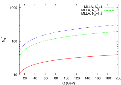
Figure 1: MLLA (8) medium-modified average multiplicity as a function of $Q=E\Theta$ in the vacuum ($N_{s}=1$) and in the medium ($N_{s}=1.6$ and $N_{s}=1.8$) for $n_{f}=3$.

The medium-modified MLLA gluon to quark average multiplicity ratio, $r=N_{g}/N_{q}=N_{g}^{h}/N_{q}^{h}$, following from (8) and (3) reads

$$r=r_{0}\left[1-r_{1}\frac{\gamma_{0}}{\sqrt{N_{s}}}+{\cal O}\left(\frac{\gamma_{0}^{2}}{N_{s}}\right)\right],\;r_{0}=\frac{N_{c}}{C_{F}},$$ (9)

where we introduced the coefficient $r_{1}=a_{1}-\tilde{a}_{1}$ in the term suppressed by $\gamma_{0}/\sqrt{N_{s}}$ as $N_{s}>1$. Therefore, if compared with its behavior at $N_{s}=1$, we check, as expected from the model [3], that $r$ becomes closer to its asymptotic DLA limit $r_{0}=N_{c}/C_{F}=9/4$, as depicted in Fig. 2. Setting $N_{s}=1$ in (9), one recovers the appropriate limits in the vacuum [4, 9, 10]. Finally, the gluon jets are still more active than the quark jets in producing secondary particles and the shape of the curves are roughly the same.

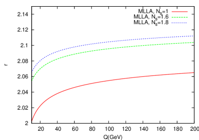
Figure 2: MLLA ratio $r$ (9) as a function of $Q=E\Theta$ in the vacuum ($N_{s}=1$) and in the medium ($N_{s}=1.6$ and $N_{s}=1.8$) for $n_{f}=3$.

The normalized second multiplicity correlator $A_{2}=\langle{N_{A}}({N_{A}}-1)\rangle/N_{A}^{2}$ defines the width of the multiplicity distribution and is related to its dispersion by the formula $D_{A}^{2}=(A_{2}-1)N_{A}^{2}+N_{A}$ [9]. These moments, which are less inclusive than the average multiplicity, prove to be ${\cal K}$-independent and therefore provide a pure test of multiparticle production. The medium-modified system of two-coupled evolution equations for this observable follows from the MLLA master equation for the azimuthally averaged generating functional [4] and can be written in the convenient form

$$\frac{d}{dY}(N_{g}^{(2)}-N_{g}^{2})\!\! \!\!=\!\! \!\!\int_{0}^{1}dx\gamma_{0}^{2}\Phi_{g}^{g}\left[N_{g}^{(2)}(Y+\ln x)\!+\!\Big{(}N_{g}^{(2)}(Y+\ln(1-x))-N_{g}^{(2)}(Y)\Big{)}\right.$$ (12)

$$\left.\hskip 14.22636pt+\Big{(}N_{g}(Y+\ln x)-N_{g}(Y)\Big{)}\Big{(}N_{g}(Y+\ln(1-x))-N_{g}(Y)\Big{)}\right]$$

$$\hskip-28.45274pt+n_{f}\!\!\int_{0}^{1}dx\gamma_{0}^{2}\Phi_{g}^{q}\left[2\Big{(}N_{q}^{(2)}(Y+\ln x)\!-\!N_{q}^{2}(Y+\ln x)\Big{)}\!-\!\Big{(}N_{g}^{(2)}(Y)\!-\!N_{g}^{2}(Y)\Big{)}\right.$$

$$\!\!+\!\! \!\!\left.\Big{(}2N_{q}(Y+\ln x)-N_{g}(Y)\Big{)}\Big{(}2N_{q}(Y+\ln(1-x))-N_{g}(Y)\Big{)}\right],$$ (13)

$$\frac{d}{dY}(N_{q}^{(2)}-N_{q}^{2})\!\! \!\!=\!\! \!\!\int_{0}^{1}dx\gamma_{0}^{2}\Phi_{q}^{g}\left[N_{g}^{(2)}(Y+\ln x)\!+\!\left(N_{q}^{(2)}(Y+\ln(1-x))-N_{q}^{(2)}(Y)\right)\right.$$ (15)

$$\left.\hskip 8.5359pt+2\Big{(}N_{g}(Y+\ln x)-N_{q}(Y)\Big{)}\Big{(}N_{q}(Y+\ln(1-x))-N_{q}(Y)\Big{)}\right],$$

which proves to be more suitable for obtaining analytical solutions in the following. We use a new method to compute solutions at MLLA by replacing $N_{A}^{(2)}=A_{2}N_{A}^{2}$ on both sides of the expanded equations at $x\sim 1-x\sim 1$. The notations in (13,15) follow the same logic as those in (5,6). Applying the analysis that led to the system (5,6), we obtain from (13,15)

$$\frac{d^{2}}{dY^{2}}\left(N^{(2)}_{g}-N_{g}^{2}\right)\! \!=\! \!\gamma_{0}^{2}\left(N_{s}-a_{1}\frac{d}{dY}\right)N^{(2)}_{g}+(a_{1}-b_{1})\gamma_{0}^{2}\frac{d}{dY}N_{g}^{2},$$ (16)

$$\frac{d^{2}}{dY^{2}}\left(N^{(2)}_{q}-N_{q}^{2}\right)\! \!=\! \!\frac{C_{F}}{N_{c}}\gamma_{0}^{2}\left(N_{s}-\tilde{a}_{1}\frac{d}{dY}\right)N^{(2)}_{g},$$ (17)

where

$$b_{1}=\frac{1}{4N_{c}}\left[\frac{11}{3}N_{c}-4\frac{T_{R}}{N_{c}}\left(1-2\frac{C_{F}}{N_{c}}\right)^{2}\right].$$

The constant $N_{s}$ only affects the leading double logarithmic term of the equations. The terms proportional to $a_{1}$, $(a_{1}-b_{1})$ and $\tilde{a}_{1}$ are hard vacuum corrections, which partially account for energy conservation, indeed $\gamma_{0}^{2}\frac{dN}{dY}\approx\sqrt{N_{s}}\gamma_{0}^{3}$ and the relative correction to DLA is ${\cal O}(\sqrt{\alpha_{s}/N_{s}})$.

Setting $N^{(2)}_{g}=G_{2}N_{g}^{2}$ in (16) and making use of (8), the system can be solved iteratively by taking terms up to ${\cal O}(\alpha_{s})$ into consideration. The analytical solution reads,

$$G_{2}-1=\frac{1-\displaystyle{\left(\frac{2}{3}a_{1}+2b_{1}\right)\frac{\gamma_{0}}{\sqrt{N_{s}}}}+{\cal O}\left(\frac{\gamma_{0}^{2}}{N_{s}}\right)}{3-(4a_{1}-\beta_{0})\displaystyle{\frac{\gamma_{0}}{\sqrt{N_{s}}}}+{\cal O}\left(\frac{\gamma_{0}^{2}}{N_{s}}\right)},$$ (18)

while its expansion in the form $1+\gamma_{0}/\sqrt{N_{s}}$ leads to

$$G_{2}-1\approx\frac{1}{3}-c_{1}\frac{\gamma_{0}}{\sqrt{N_{s}}}+{\cal O}\left(\frac{\gamma_{0}^{2}}{N_{s}}\right),$$ (19)

where the linear combination of color factors can be written in the form

$$c_{1}=\frac{1}{4N_{c}}\!\left(\!\frac{55}{9}-4\frac{T_{R}}{N_{c}}+\frac{112}{9}\frac{T_{R}}{N_{c}}\frac{C_{F}}{N_{c}}-\frac{32}{3}\frac{T_{R}}{N_{c}}\frac{C_{F}^{2}}{N_{c}^{2}}\right).$$ (20)

We use (19) and (9) and substitute $N^{(2)}_{q}=Q_{2}N_{q}^{2}$ into (17) such that the solution reads

$$Q_{2}-1\approx\frac{N_{c}}{C_{F}}\left(\frac{1}{3}-\tilde{c}_{1}\frac{\gamma_{0}}{\sqrt{N_{s}}}\right)+{\cal O}\left(\frac{\gamma_{0}^{2}}{N_{s}}\right),$$ (21)

where we obtain the combination of color factors

$$\tilde{c}_{1}=\frac{1}{4N_{c}}\!\left(\!\frac{55}{9}+\frac{4}{9}\frac{T_{R}}{N_{c}}\frac{C_{F}}{N_{c}}-\frac{8}{3}\frac{T_{R}}{N_{c}}\frac{C_{F}^{2}}{N_{c}^{2}}\right).$$ (22)

Setting $N_{s}=1$ in (19) and (21) we get a perfect agreement with the vacuum results [9]. In Fig. 3 and Fig. 4, we compare our results for the medium-modified second multiplicity correlators (19) and (21) with predictions in the vacuum ($N_{s}=1$) [9] in the limiting spectrum approximation inside the typical range $10\leq Q(\text{GeV})\leq 200$ for RHIC and LHC phenomenology.

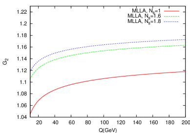
Figure 3: MLLA second multiplicity correlator inside a gluon jet (19) as a function of $Q=E\Theta$ in the vacuum ($N_{s}=1$) and in the medium ($N_{s}=1.6$ and $N_{s}=1.8$ for $n_{f}=3$.

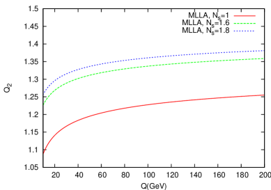
Figure 4: MLLA second multiplicity correlator inside a quark jet (21).

Similarly to the MLLA ratio $r(N_{s})$, Eq. (9), the hard corrections ${\cal O}(\gamma_{0})$ are suppressed by a factor $1/\sqrt{N_{s}}$. As expected from the model, we check that these results approach their DLA limits when $N_{s}$ increases; moreover, the multiplicity fluctuations of individual events must be larger for quark jets as compared to gluon jets just like in the vacuum [9]. Another interesting feature of these observables concerns the shape of the curves. They are roughly identical and prove not to depend on the medium parameter $N_{s}$. Moreover, there exists evidence for a flattening of the slopes as the hardness of the jet $Q=E\Theta$ increases for $N_{s}\geq 1$ (vacuum and medium). This kind of scaling behavior is known as the Koba-Nielsen-Olsen (KNO) scaling [11]: it was discovered by Polyakov in quantum field theory [12] and experimentally confirmed by $e^{+}e^{-}$ measurements [13] for the second and higher order multiplicity correlators.

In this paper we have dealt with the medium-modified average multiplicity and the medium-modified second multiplicity correlator in quark and gluon jets at RHIC and LHC energy scales. The starting point of our calculations is based on the Borghini-Wiedemann work [3], which models parton energy loss in a nuclear medium. The average multiplicity is found to be enhanced by the factor $\sqrt{N_{s}}$ acting on the exponential leading contribution (8); this leads in particular to the rescaling of the anomalous dimension $\gamma_{\text{med}}$ ($\gamma\to\gamma_{\text{med}}\approx\sqrt{N_{s}}\gamma_{0}$) or equivalently, to the enhancement of the in medium coupling constant. Since hard corrections are suppressed by the extra factor $1/\sqrt{N_{s}}$, it is straightforward to check that $r$, $G_{2}$ and $Q_{2}$ approach the asymptotic DLA limits $r_{0}=N_{c}/C_{F}$, $G_{2}=4/3$ and $Q_{2}=1+N_{c}/3C_{F}$ [4] when $N_{s}$ increases. The previously mentioned KNO-scaling experienced by $G_{2}$ and $Q_{2}$ proves no special sensibility to the model and should normally hold like in the vacuum.

Finally, since these results are model-dependent, they may still be improved in the future, specially after the $N_{s}$-dependence of the non-singular parts of the splitting functions (4) has been exactly computed.

Perspective: Many experimental characterizations of the medium-modified intrajet structure in heavy-ion collisions at RHIC and at the LHC require a soft momentum cut-off $p_{T}^{\text{cut}}$, with $Q>p_{T}^{\text{cut}}$ to remove the effects of the high multiplicity background. In [3], the soft background was subtracted by integrating the single inclusive differential distribution $\frac{dN}{d\ln p_{T}}$ (“hump-backed plateau”) over the range $Q\geq p_{T}\geq p_{T}^{\text{cut}}$, with $p_{T}^{\text{cut}}>\Lambda_{QCD}$. Accordingly, the equivalent computation should be performed for the second multiplicity correlator by integrating the double differential inclusive distribution (two-particle correlation) $\frac{d^{2}N}{d\ln p_{1,T}d\ln p_{2,T}}$ over $p_{i,T}$, with the lower bounds of integration $p_{i,T}^{\text{cut}}>\Lambda_{QCD}$ ($i=1,2$). Imposing such a cut-off in our calculations will affect the normalization rather than the behavior and the shape of these observables as a function of $N_{s}$ and the jet energy scale of the process $Q$ [14].

References

[1]
K. Adcox et al. (PHENIX Collab.), Phys. Rev. Lett. 88
(2002) 022301;
S.S. Adler et al. (PHENIX Collab.),
Phys. Rev. Lett. 91 (2003) 072301;
C. Adler et al. (STAR Collab.),
Phys. Rev. Lett 89 (2002) 202301.
[2]
F. Arleo, hep-ph/0810.1193 and references therein;
S. Peigné & A.V. Smilga, hep-ph/0810.5702.
[3]
N. Borghini & U.A. Wiedemann, hep-ph/0506218.
[4]
Yu.L. Dokshitzer, V.A. Khoze, A.H. Mueller & S.I. Troyan, Basics of
Perturbative QCD, Editions Frontières, Paris (1991).