Emission-lines calibrations of the Star Formation Rate from the Sloan Digital Sky Survey

Abstract

Aims. Up to now, the study of the star formation rate in galaxies has been mainly based on the H$\alpha$ emission-line luminosity. However, this standard calibration cannot be applied at all redshifts given one instrumental setup. Surveys based on optical spectroscopy do not observe the H$\alpha$ emission line at redshifts higher than $z\sim 0.5$. Our goal is to study existing star formation rate calibrations and to provide new ones, still based on emission-line luminosities, which can be applied for various instrumental setups.

Methods. We use the SDSS public data release DR4, which gives star formation rates and emission-line luminosities of more than $100\,000$ star-forming galaxies observed at low redshifts. We take advantage of this statistically significant sample in order to study the relations, based on these data, between the star formation rate and the luminosities of some well-chosen emission lines. We correct the emission-line measurements for dust attenuation using the same attenuation curve as the one used to derive the star formation rates.

Results. We confirm that the best results are obtained when relating star formation rates to the H$\alpha$ emission line luminosity, itself corrected for dust attenuation. This calibration has an uncertainty of $0.17$ dex. We show that one has to check carefully the method used to derive the dust attenuation and to use the adequate calibration: in some cases, the standard scaling law has to be replaced by a more general power law. When data is corrected for dust attenuation but the H$\alpha$ emission line not observed, the use of the H$\beta$ emission line, if possible, has to be preferred to the [Oii]$\lambda$3727 emission line. In the case of uncorrected data, the correction for dust attenuation can be assumed as a constant mean value but we show that such method leads to poor results, in terms of dispersion and residual slope. Self-consistent corrections such as previous studies based on the absolute magnitude give better results in terms of dispersion but still suffer from systematic shifts, and/or residual slopes. The best results with data not corrected for dust attenuation are obtained when using the observed [Oii]$\lambda$3727 and H$\beta$ emission lines together. This calibration has an uncertainty of $0.23$ dex.

1 Introduction

Massive ongoing spectroscopic surveys of the high-redshift Universe allow us to draw a new picture of how the galaxies evolve through cosmic times. Many physical properties are used as tracers of the evolutionary stage and the past history of one galaxy (e.g. stellar mass, metallicity, amount of dust, star formation rate). Thanks to extensive works on stellar population models (Bruzual & Charlot, 2003; Fioc & Rocca-Volmerange, 1997) and photo-ionization models (Charlot & Longhetti, 2001), most of these parameters can now be well recovered from rest-frame optical spectroscopic observations, using all information available from the stellar continuum and absorption- or emission-line measurements.

Unfortunately, these models often require a better signal-to-noise ratio, wavelength coverage, and/or spectral resolution than the ones available on recent deep surveys (e.g. VVDS: Le Fèvre et al., 2005; zCOSMOS: Lily et al. 2007). Thus, a simpler approach is to use instead emission-line diagnostics that would be calibrated on high quality samples, taken from local Universe surveys (e.g. 2dFGRS: Colless et al., 2001; SDSS: York et al., 2000). This approach has already been extensively used with older data to recover metallicities with oxygen-to-hydrogen (McGaugh, 1991; Kewley & Dopita, 2002) or nitrogen-to-hydrogen (Pettini & Pagel, 2004; van Zee et al., 1998) line ratios, dust content with the H$\alpha$/H$\beta$ Balmer decrement (Seaton, 1979; Calzetti, 2001), or star formation rates with the H$\alpha$ or [Oii]$\lambda$3727 emission-line luminosities (Kennicutt, 1998; Kewley et al., 2004).

Recently, the star formation rates of $>100\,000$ SDSS star-forming galaxies have been estimated using the CL01 method (Charlot & Longhetti, 2001) which takes into account all information available in emission-line measurements (Brinchmann et al., 2004). Then, the emission-line measurements of the same galaxies have also been made publicly available. We can thus use this large amount of data to derive new good quality calibrations of the star formation rates (hereafter SFR) from emission-line luminosities.

The standard calibration of the SFR versus the H$\alpha$ luminosity is based on a very simple scaling relation, driven by the amount of H$\alpha$ recombination photons being directly proportional to the intensity of the ionizing source, i.e. the amount of young, hot stars, which the SFR is an indicator of (Kennicutt, 1998). The only drawback to this simple assumption is that the H$\alpha$ luminosity has to be corrected for dust attenuation.

As shown by Kewley et al. (2004), the calibration of the SFR versus the [Oii]$\lambda$3727 luminosity is not only more affected by dust attenuation, but also depends on metallicity, since interstellar medium with higher gas-phase metallicities produces less [Oii]$\lambda$3727 photons because of increased oxygen cooling. Starting from this result, they have derived new calibrations of the SFR versus [Oii]$\lambda$3727 luminosity which take into account the metallicity. The idea was to calibrate the [Oii]$\lambda$3727/H$\alpha$ emission-line ratio versus the metallicity, and then to use it to recover the SFR from the H$\alpha$ luminosity, itself derived from the [Oii]$\lambda$3727 luminosity. The dependence on the metallicity of the [Oii]$\lambda$3727/H$\alpha$ emission-line ratio, or more generally the [Oii]$\lambda$3727 based SFR calibrations, has been later confirmed by Mouhcine et al. (2005) and Bicker & Fritze-v. Alvensleben (2005).

Recently Moustakas et al. (2006) and Weiner et al. (2007) have derived a new calibration of the SFR of galaxies versus [Oii]$\lambda$3727 luminosity. They take care of the effect of the metallicity with a slightly different approach, by parametrizing their calibration in terms of the $B$-band luminosity, which can be used as a rough metallicity indicator because of the metallicity-luminosity relation (Lequeux et al., 1979; Skillman et al., 1989; Richer & McCall, 1995; Lamareille et al., 2004; Tremonti et al., 2004; Lamareille et al., 2006).

We point out that these previous studies base their new calibrations on either a direct estimate or a secondary indicator (e.g. rest-frame luminosity) of the metallicity, which in both cases suffers from intrinsic uncertainties and degeneracies (see Kewley & Ellison, 2008 for a detailed discussion on the uncertainties of metallicity calibrations, or Lamareille et al. 2004 for a discussion on the dispersion of the luminosity-metallicity relation). Moreover, some of these previous works also assume that the dust attenuation is known, whereas it is difficult to estimate this quantity when H$\alpha$ emission line is not measured (which is the case when one wants to used [Oii]$\lambda$3727 instead to derive SFR).

The paper is organized as follows: we first present the sample we have used and the selection we applied to it (Sect. 2), then we calibrate the SFR as a function of emission-line luminosities when a correction for dust attenuation is available (Sect. 3), or when it is not available (Sect. 4). We finally draw some conclusions (Sect. 5).

2 Description of the sample

The physical properties of a total of $567\,486$ galaxy spectra inside SDSS Data Release 4 (DR4, Adelman-McCarthy et al., 2006) have been made publicy available on the following website: http://www.mpa-garching.mpg.de/SDSS/. Taking advantage of this huge amount of data, we made a sub catalog with the SFR, the emission-line measurements, the spectral classification and the metallicities of a sub sample of galaxies. The selection will be described later in this section as we first describe, for the benefit of the reader, the main ingredients of the methods used to derive the physical parameters.

2.1 Physical properties

The spectral properties of SDSS galaxies have been measured with “platefit” software by Tremonti et al. (2004). For each spectrum, they perform a careful subtraction of the stellar continuum and absorption lines by fitting a linear combination of single stellar population models of different ages (Bruzual & Charlot, 2003). Then they fit all emission lines at the same time as a unique nebular spectrum in which each line is modeled by a Gaussian. Thanks to the subtraction of the stellar component, Balmer emission lines are automatically corrected for underlying absorption. We note that the [Oii]$\lambda$3727 line that we use in this study is the sum of two Gaussians of the same width modeling the [Oii]$\lambda\lambda$3726,3729 doublet. The AGN classification is based on the [Oiii]$\lambda$5007/H$\beta$ vs. [Nii]$\lambda$6584/H$\alpha$ emission-line diagnostic diagram and has been performed by Kauffmann et al. (2003a).

The SFR and gas-phase oxygen abundances have been computed from emission-lines fluxes using the Charlot & Longhetti (2001, hereafter CL01) method by Brinchmann et al. (2004) and Tremonti et al. (2004) respectively. This method compares all emission-lines fluxes together to a set of theoretical nebular spectra, which are modeled with five parameters: the metallicity, the ionization degree, the dust-to-metal ratio, the dust attenuation, and the SFR efficiency factor. For each galaxy, one estimate of each observed parameter is computed through a Bayesian approach (see Brinchmann et al., 2004 for more details). We note that the SFRs are computed assuming the Kroupa (2001) initial mass function (IMF). One may scale the SFR estimates discussed in this paper to the Salpeter (1955) IMF by multiplying them by a factor $1.5$ (or by adding $0.176$ dex to their logarithm), and to the Chabrier (2003) IMF by multiplying them by a factor $0.88$ (or by subtracting $0.056$ dex to their logarithm). The CL01 SFR will be used as the reference SFR throughout this study.

We compute the luminosity $L$ of each line starting from its measured flux $F$, and the redshift $z$ of the galaxy, using the following equation:

$$\begin{array}[]{c}L=4\pi\left(\frac{c}{H_{\mathrm{0}}}\cdot(1+z)\cdot\int_{0}^{z}f(z^{\prime})^{-1/2}dz^{\prime}\right)^{2}\times F\\ f(z^{\prime})=(1+z^{\prime})^{2}(1+\Omega_{\mathrm{m}}z^{\prime})-\Omega_{\Lambda}z^{\prime}(2+z^{\prime})\end{array}$$ (1)

The luminosities are calculated with the same cosmology based on WMAP results (Spergel et al., 2003) as the one used by Brinchmann et al. (2004) to estimate the SFR: $H_{\mathrm{0}}=70$ km s^-1 Mpc^-1, $\Omega_{\Lambda}=0.7$ and $\Omega_{\mathrm{m}}=0.3$. We note that all the calibrations provided in this study are independent of the cosmology. They indeed compare SFR and emission-line luminosities which are affected in the same way by the distance modulus.

Finally, we have cross-matched this catalog with the VAGC catalog (Blanton et al., 2005) to get the $k$-corrected absolute magnitudes which are used in this study. The absolute magnitude in the $B$-band is derived from SDSS $u^{\prime}$- and $g^{\prime}$-bands using Eq. 1 of Moustakas et al. (2006).

2.2 Dust attenuation

We will use the following notations in all this work: the observed flux of the three emission lines used in this study are designed by the name of the line: H$\alpha$, H$\beta$ and [Oii] (stands for [Oii]$\lambda$3727). The intrinsic flux corrected for dust attenuation is designed by a superscript i: H$\alpha^{\mathrm{i}}$, H$\beta^{\mathrm{i}}$ and [Oii]ⁱ. The attenuation law is designed by the function $\tau(\lambda)$, and the effective dust attenuation in $V$-band by the symbol $\tau_{V}$. For simplification purposes, we also note: $\tau(V)=\tau(5500\,\mbox{\AA})$ ($V$-band), $\tau(\beta)=\tau(4861\,\mbox{\AA})$, $\tau(\alpha)=\tau(6563\,\mbox{\AA})$, and $\tau(\mathrm{O}\mathsc{ii})=\tau(3727\,\mbox{\AA})$. The intrinsic flux $f_{\lambda}^{\mathrm{i}}(\lambda)$ at any wavelength $\lambda$ as a function of the observed flux $f_{\lambda}(\lambda)$ is given by the following equation:

$$f_{\lambda}^{\mathrm{i}}(\lambda)=f_{\lambda}(\lambda)\cdot\exp\left(\frac{\tau_{V}}{\tau(V)}\cdot\tau(\lambda)\right)$$ (2)

We compute the dust attenuation by comparing the observed to the intrinsic H$\alpha$/H$\beta$ emission-line ratios, using the following equation:

$$\tau_{V}^{\mathrm{Balmer}}=\frac{\ln(\mathrm{H}\alpha/\mathrm{H}\beta)-\ln(\mathrm{H}\alpha^{\mathrm{i}}/\mathrm{H}\beta^{\mathrm{i}})}{\tau(\beta)-\tau(\alpha)}\cdot\tau(V)$$ (3)

In the following work, we use the standard case B recombination ratio (hereafter standard intrinsic Balmer ratio): $\mathrm{H}\alpha^{\mathrm{i}}/\mathrm{H}\beta^{\mathrm{i}}=2.85$ (Osterbrock, 1989) and the Charlot & Fall (2000) mean attenuation curve: $\tau(\lambda)\propto\lambda^{-0.7}$. The choice of this curve is made to be consistent with the setup used to compute the SFRs in the SDSS DR4 data (the SFR is computed self-consistently with correction for dust attenuation).

The dust attenuation recovered with an assumed constant intrinsic Balmer ratio ($\tau_{V}^{\mathrm{Balmer}}$) does not take into account the variations of this ratio with other physical parameters (e.g. metallicity). We thus also use in this study the true dust attenuation recovered with CL01 models by Brinchmann et al. (2004). We design it by the symbol $\tau_{V}^{\mathrm{CL01}}$. The intrinsic flux corrected for dust attenuation using this parameter is designed by a superscript $iC$: H$\alpha^{\mathrm{iC}}$, H$\beta^{\mathrm{iC}}$ and [Oii]^iC.

Finally, another way to estimate the dust attenuation is to compare the observed colors of the galaxies to a library of stellar population synthesis models (hereafter SED fitting). This work has been carried on with Bruzual & Charlot (2003) models on SDSS galaxies by Kauffmann et al. (2003b), who provide an estimate of the continuum attenuation in the $z$-band ($A_{z}$) with Charlot & Fall (2000) attenuation curve. It is straightforward to convert the $A_{z}$ parameter to $\tau_{V}$ using the following formula:

$$\tau_{V}^{\mathrm{SED}}=\frac{A_{z}}{1.086}\cdot\left(\frac{5500}{8800}\right)^{-0.7}\cdot\frac{1}{A_{\star}/A_{\mathrm{g}}}$$ (4)

Please note that the $1.086$ factor is the conversion from magnitudes to opacities and $A_{\star}/A_{\mathrm{g}}$ is the mean ratio between the dust attenuation affecting stars (which dominate the colors of the galaxies) and the one affecting gas. The dust attenuation estimated from SED fitting is characterized by a high uncertainty but might be used in a statistical way.

2.3 Sample selection

Thanks to the spectral classification provided by Kauffmann et al. (2003a), we select only star-forming galaxies and remove all AGN from our sample. In the whole study, we additionally remove all galaxies for which H$\alpha$ and H$\beta$ emission lines (used for estimating the dust attenuation) are not measured with a signal-to-noise ratio of at least $5$. We apply the same selection to the [Oii] emission line in order to derive the calibrations in which this line is involved. We note that the signal-to-noise ratios have been corrected according to the values provided in the SDSS/MPA website (based on the analysis of duplicated observations): they have been divided by $2.473$ for H$\alpha$ line, $1.882$ for H$\beta$ line and $2.199$ for [Oii] line. We also kept only galaxies with an available estimate of $\tau_{V}^{\mathrm{CL01}}$. This selection was applied to remove a number of spectra with unreliable flux measurements. Please note that a number of objects may show a negative $\tau_{V}^{\mathrm{Balmer}}$ estimate. This is due to statistical variations around the wrong assumption of a constant intrinsic Balmer ratio: these objects have not to be removed.

Finally, some objects in SDSS DR4 catalog have been observed twice or more. We decided to keep only one observation of each duplicated galaxy by selecting the one with the best signal-to-noise ratio on the H$\alpha$ emission line. We end up with $123\,713$ and $84\,733$ star-forming galaxies for H$\alpha$-based and [Oii]-based studies respectively.

All the parameters used in this study (SFR, metallicity, dust attenuation) are the median estimates.

2.4 Properties of the studied sample

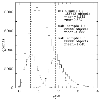
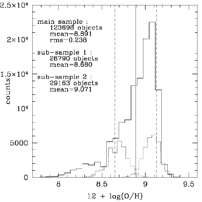
Figure 1: This plot shows the histogram of the dust attenuation (left), or of the gas-phase oxygen abundance (right), both estimated with the CL01 method, for the star-forming galaxies in the SDSS DR4 data. The solid vertical line shows the mean value of the distribution, and the dashed vertical lines the 1-$\sigma$ tails. The values are given in the plot. The two dotted histograms shows the distribution of our two sub-samples (see text for details).

Fig. 1 (left) shows the distribution of the effective dust attenuation in the $V$-band (estimated with the CL01 method) in the sample we have obtained. The mean value is $1.21$ and the dispersion is $0.637$. We note that this values are obtained with the selection on H$\alpha$ and H$\beta$ lines only. The new mean and dispersion when we add the selection on the [Oii] line are $1.10$ and $0.547$ respectively. Fig. 1 (right) shows the distribution of the gas-phase oxygen abundance in the same sample (for objects with an available measurement of this parameter). The mean value is $8.89$ with a dispersion of $0.24$ ($8.88$ mean value with a dispersion of $0.21$ if the selection on the [Oii] line is applied).

Fig. 1 also shows the distributions of four sub-samples (two in each panel). These sub-samples have been randomly selected from the main sample, forcing their mean values to be closest as possible to the mean value of the main sample plus or minus its dispersion, and their dispersion to be half the dispersion of the main sample. We end up with four sub-samples: low dust attenuation, high dust attenuation, low metallicity, and high metallicity. They will be used to test the calibrations on samples with different dust properties.

3 SFR calibration with an available dust estimate

We present in this section emission-line calibrations of the SFR based on data already corrected for dust attenuation. We first focus in Sect. 3.2 on data with dust attenuation estimated from the Balmer decrement, which is the common case in the literature. We then study in Sect. 3.3 the different calibrations we obtain when using the dust attenuation estimated from the CL01 method or SED fitting.

3.1 Base theory

The common way to calibrate the SFR against one emission line luminosity (e.g. H$\alpha$) is a simple scaling relation of the following form:

$$\mathrm{SFR}=L(\mathrm{H}\alpha)/\eta_{\mathrm{H}\alpha}$$ (5)

This formula, where $\eta_{H\alpha}$ is the efficiency factor, reproduces the simple relation between the amount of ionizing photons (the SFR) and the emission-line luminosity. However, it has been already shown that the H$\alpha$ efficiency factor depends on other physical properties of the galaxies: Charlot & Longhetti (2001) have shown that $\eta_{H\alpha}$ depends on the metallicity, metal-rich stars being less luminous and thus producing less H$\alpha$ photons in the interstellar medium for a same SFR. More recently, Brinchmann et al. (2004) have shown that $\eta_{H\alpha}$ is also linked to the stellar mass of SDSS galaxies, massive galaxies producing less H$\alpha$ photons than dwarfs for a given SFR. We note that these two results are obviously linked by the mass-metallicity relation (Tremonti et al., 2004; Lamareille et al., 2008). Fortunately, Brinchmann et al. (2004) have also shown that this effect is canceled by the commonly used wrong assumption of a constant intrinsic H$\alpha$/H$\beta$ intrinsic Balmer ratio. In fact this ratio increases with metallicity, ending up with an overestimate of the dust attenuation for metal-rich galaxies. This latter effect almost exactly compensates the decrease of $\eta_{H\alpha}$ when metallicity increases.

Nevertheless, we decided to adopt a more general approach using a power-law as described by the following formula:

$$\log(\mathrm{SFR})=\epsilon_{\mathrm{H}\alpha}\log L(\mathrm{H}\alpha)-\log(\eta_{\mathrm{H}\alpha})$$ (6)

The parameter $\epsilon_{\mathrm{H}\alpha}$ is the exponent of the power law. The simple calibration described by Eq. 5 corresponds to the $\epsilon_{\mathrm{H}\alpha}=1$ special case. We show in the following sections that this more general approach is not mandatory for the cases with a dust attenuation estimated from the Balmer decrement ($\epsilon_{\mathrm{H}\alpha}$ is very close to $1$), but that it is useful in other cases.

We note that the correlation between dust attenuation and metallicity (Cortese et al., 2006; Mouhcine et al., 2005) also has an effect on the slope. However the goal of our work in not to study in details such phenomenon.

In the following sections, the efficiency factors are expressed in erg s^-1 (M_⊙ yr^-1)^-1 units and the exponents of the power laws are unit-less. All fits are least square fits with errors in $x$ and $y$. The errors on the fitted parameters are given by the rms of 40 bootstrap estimates. The term “dispersion” relates to the rms of the residuals around the fitted calibrations, the term “shift” to the mean of these residuals. The given residual slopes are unit-less.

3.2 Dust estimated from the Balmer decrement

We now present possible calibrations of the SFR based on data corrected with dust estimated from the Balmer decrement (see Eq. 3). We remind the reader that the results presented in this subsection are valid only if we correct the observed flux for dust attenuation using Eqs. 2 and 3, i.e. making the wrong assumption that the intrinsic Balmer ratio is constant over all the range of stellar masses.

3.2.1 Improved standard calibrations

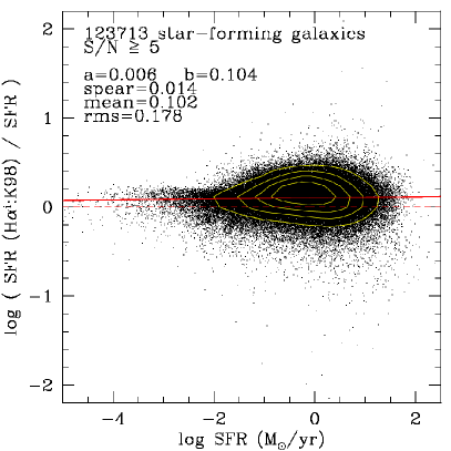
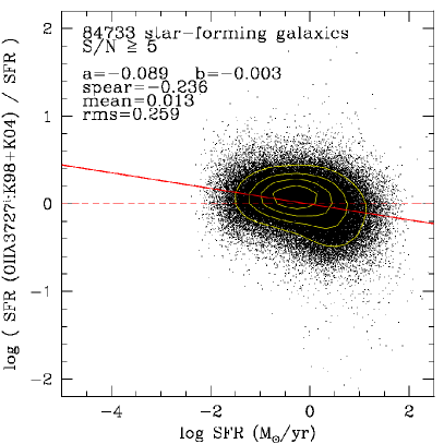
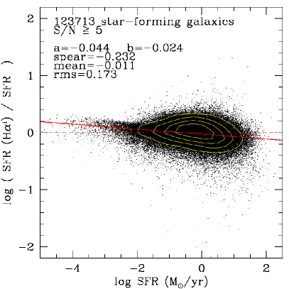
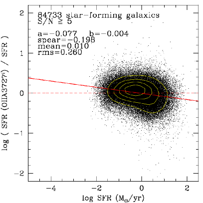
Figure 2: These four plots show the residuals of the SFR recovered from an emission-line calibration as compared to the reference CL01 SFR, for star-forming galaxies in the SDSS DR4 data. This comparison is shown as the logarithm of the ratio between the derived and the reference SFR, as a function of the logarithm of the reference SFR (in M_⊙/yr). The number of objects used in the comparison, the shift, the dispersion, and the Spearman rank correlation coefficient are given in the plot. The dashed horizontal line is the $y=0$ curve, the solid line is the $y=a\cdot x+b$ curve where $a$ and $b$ are the parameters of the linear regression given in the plot. Isodensity contours are overplotted in white. The studied calibrations are: top-left: Kennicutt (1998) H$\alpha^{\mathrm{i}}$; top-right: Kennicutt (1998) (corrected by Kewley et al., 2004) [Oii]ⁱ; bottom-left: our improved H$\alpha^{\mathrm{i}}$ calibration; bottom-right: our improved [Oii]ⁱ calibration.

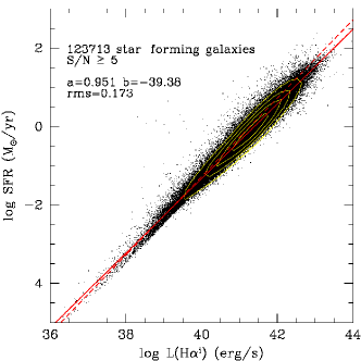
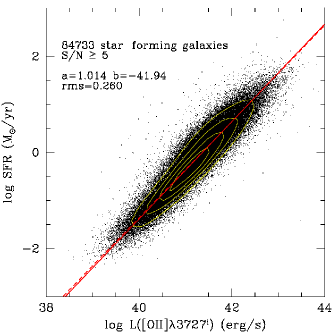
Figure 3: Relation between the SFR (logarithm of M_⊙/yr) and the H$\alpha^{\mathrm{i}}$ (left) or [Oii]ⁱ (right) emission lines luminosities (logarithm of erg/s) for star-forming galaxies in the SDSS DR4 data. The solid line is a least-square fit to the data (errors on $x$ and $y$). The dashed line is the Kennicutt (1998) calibration corrected to our assumed IMF, and corrected for dust by Kewley et al. (2004) on the right panel. Isodensity contours are overplotted in white.

Kennicutt (1998) has developed two calibrations of the SFR versus H$\alpha^{\mathrm{i}}$ or the [Oii]ⁱ emission lines which are now widely used in the literature. We take advantage of the SDSS DR4 data to test these two calibrations as compared to the high quality CL01 estimate of the SFR. We also derive two new improved calibrations based on Eq. 6 rather than Eq. 5.

Fig. 2 (top-left) shows the comparison between the CL01 SFR and the one recovered with the standard Kennicutt (1998) H$\alpha^{\mathrm{i}}$ calibration, which uses $\log(\eta_{\mathrm{H}\alpha}^{\mathrm{i}})=41.28$ if we scale their results to our adopted IMF. We find a good agreement: the dispersion is $0.17$ dex, which is very similar to the minimum uncertainty associated to the CL01 SFR estimates (i.e. $0.16$ dex). Thus, we confirm that the H$\alpha$ emission line luminosity alone is sufficient to recover almost perfectly the SFR.

However, we see that the reduced efficiency factor and the dust attenuation overestimate do not exactly cancel each other on the massive end of the sample, which induces a mean of the residuals of $+0.1$ dex. One might decide to subtract $0.1$ dex to the Kennicutt (1998) calibration in order to find a null mean of the residuals, or we can try to derive an improved calibration.

Fig. 3 (left) shows our improved calibration for the correlation between the H$\alpha^{\mathrm{i}}$ emission-line luminosity and the SFR in SDSS DR4 data. We find the following best fit values:

$$\left\{\begin{array}[]{ccl}\log\eta_{\mathrm{H}\alpha}^{\mathrm{i}}&=&39.38\pm 0.03\\ \epsilon_{\mathrm{H}\alpha}^{\mathrm{i}}&=&0.951\pm 0.001\end{array}\right.$$ (7)

One can notice that the formal errors of these two parameters are very low thanks to the large number of objects, which makes this calibration quite reliable. The uncertainty on the exponent of the power law especially tells us that this parameter is very well constrained, while not equal to $1$ as compared to all previous studies. As shown in Fig. 2 (bottom-left), the mean on the residuals is now almost null ($0.01$ dex) with the improved calibration. A small residual slope ($-0.04$) is present as the improved calibration is now less accurate for very low SFR values. This residual slope is not significant given the low Spearman rank correlation coefficient: $-0.23$.

We now consider the case where the H$\alpha$ line is not observed, or not measurable, and that we decide to use the [Oii]$\lambda$3727 emission line instead. In such case, the dust attenuation might be derived from another Balmer ratio not involving the H$\alpha$ line (e.g. H$\gamma$/H$\beta$, H$\delta$/H$\gamma$, …)

As already stated in the literature, the relation between the SFR and the [Oii] line has to be considered with caution because of the stronger dependence of this line on metallicity (compared to H$\alpha$), as well as a stronger sensibility to dust attenuation. However, as shown in Fig. 2 (top-right), we find a good agreement with the standard Kennicutt (1998) [Oii]ⁱ calibration, which uses $\log(\eta_{[\mathrm{O}\mathsc{ii}]}^{\mathrm{i}})=41.36$ if we correct their results for dust attenuation (Kewley et al., 2004) and scale them to our adopted IMF.

It seems that the effect of metallicity on the [Oii] line does not produce any systematic shift and only leads to a higher dispersion: $0.25$ dex. To be more precise, the three effects of the metallicity on the relative strength of the [Oii] line, on the efficiency factor, and on the estimate of the dust attenuation exactly compensate in order to produce a exponent of the power law very close to unity.

Fig. 3 (right) shows our improved calibration in the correlation between the [Oii]ⁱ emission-line luminosity and the SFR in SDSS DR4 data. We find the following best-fit values:

$$\left\{\begin{array}[]{ccl}\log\eta_{[\mathrm{O}\mathsc{ii}]}^{\mathrm{i}}&=&41.94\pm 0.7\\ \epsilon_{[\mathrm{O}\mathsc{ii}]}^{\mathrm{i}}&=&1.014\pm 0.02\end{array}\right.$$ (8)

As expected, and as shown in Fig. 2 (bottom-right), this calibration does not produce any significant improvement compared to the Kennicutt (1998) (corrected by Kewley et al., 2004) calibration. In both cases, the observed residual slope of $-0.09$ is not significant (Spearman rank correlation coefficient of $-0.24$).

3.2.2 New calibrations

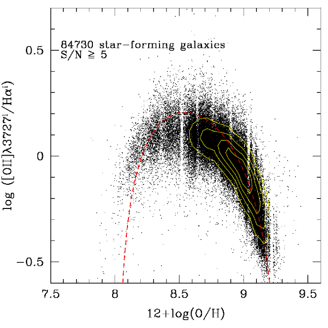
Figure 4: Relation between the [Oii]$\lambda$3727ⁱ/H$\alpha^{\mathrm{i}}$ emission line ratio and gas-phase oxygen abundance (estimated with the CL01 method) for the star-forming galaxies in the SDSS DR4 catalog. The dashed curve is a semi-empirical estimation of this relation (Kewley et al., 2004).

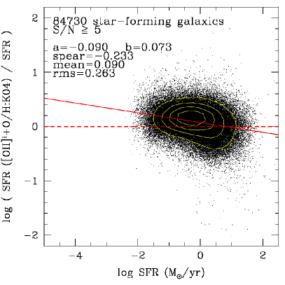
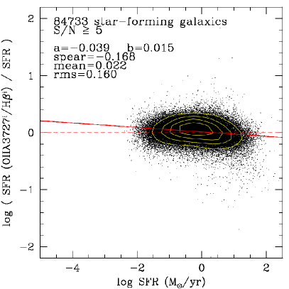
Figure 5: Same legend as in Fig. 2. The studied calibrations are: left: Kewley et al. (2004) [Oii]ⁱ with a correction for metallicity; right: our new [Oii]ⁱ+H$\beta^{\mathrm{i}}$ calibration.

As already shown in previous works (Kewley et al., 2004; Moustakas et al., 2006; Weiner et al., 2007), the best way to provide a reliable SFR vs. [Oii] calibration is to actually use the SFR vs. H$\alpha^{\mathrm{i}}$ calibration, and to calibrate either the [Oii]/H$\alpha^{\mathrm{i}}$ (observed-to-intrinsic) or the [Oii]ⁱ/H$\alpha^{\mathrm{i}}$ (intrinsic-to-intrinsic) line ratio against a well chosen parameter. Then the star formation rate is given by the following formula:

$$\log\mathrm{SFR}=\epsilon_{\mathrm{H}\alpha}^{\mathrm{i}}\left(\log L(\mathrm{[O}\mathsc{ii}\mathrm{]}^{\mathrm{i?}})-\log(\mathrm{[O}\mathsc{ii}]^{\mathrm{i?}}/\mathrm{H}\alpha^{\mathrm{i}})\right)-\log\eta_{\mathrm{H}\alpha}^{\mathrm{i}}$$ (9)

Kewley et al. (2004) has calibrated the [Oii]ⁱ/H$\alpha^{\mathrm{i}}$ line ratio against the gas-phase oxygen abundance ($12+\log(\mathrm{O}/\mathrm{H})$), ending up in an appreciable improvement of the calibration. As also shown by Mouhcine et al. (2005) with 2dFGRS data and in Fig. 4, there is indeed a robust correlation between these two parameters. The dashed line in Fig. 4 shows the relation derived semi-empirically by Kewley et al. (2004). The residuals around this relation are characterized by a mean of $-0.04$ dex and a rms of $0.1$ dex in SDSS DR4 data.

However, we see three drawbacks against the use of this relation:

• First the gas-phase oxygen abundance is not an easy parameter to derive. There are many different calibrations which can be different from each other by up to $0.5$ dex (see Kewley & Ellison, 2008, for a detailed discussion). Moreover, most of these calibrations need many emission lines to be measured and we emphasize that, in such cases, it might be easier to use directly the SFR estimated from multiple-lines fitting methods like CL01.

• Second, we already stated before that correcting the [Oii] emission line for dust attenuation requires in most common cases that the H$\alpha$ emission line is being observed: in this case one would estimate the SFR directly from the H$\alpha$ line, rather from the [Oii] line. Thus, trying to improve the [Oii] calibration with data corrected for dust attenuation is actually not applicable in most common cases.

• For the other cases (e.g. dust attenuation estimated from another Balmer ratio), we also remark that using the metallicity estimate (or any other derived parameter) to correct the calibration is not necessary. Indeed a very simple relation, which do not need a metallicity estimate, already exists between [Oii]ⁱ, H$\alpha^{\mathrm{i}}$ and H$\beta^{\mathrm{i}}$ emission lines. This simple relation is expressed by the following equation assuming the standard intrinsic Balmer ratio:

  $$\frac{[\mathrm{O}\mathsc{ii}]^{\mathrm{i}}}{\mathrm{H}\alpha^{\mathrm{i}}}=\frac{[\mathrm{O}\mathsc{ii}]^{\mathrm{i}}}{\mathrm{H}\beta^{\mathrm{i}}}/\frac{\mathrm{H}\alpha^{\mathrm{i}}}{\mathrm{H}\beta^{\mathrm{i}}}=\frac{[\mathrm{O}\mathsc{ii}]^{\mathrm{i}}}{\mathrm{H}\beta^{\mathrm{i}}}/2.85$$ (10)

We applied Eq. 15 of Kewley et al. (2004) in order to compare their metallicity- and dust-corrected calibration to the reference CL01 SFR. We have done that only for the $84\,730$ galaxies for which an estimate of the gas-phase oxygen abundance was available. Before doing that, we have corrected our available CL01 metallicities to Kewley & Dopita (2002) metallicities, using the formula in Table B3 of Kewley & Ellison (2008).

As shown in Fig. 5 (left), the Kewley et al. (2004) calibration shows a non-negligible $0.1$ dex shift. Moreover, the dispersion of the relation is $0.26$ dex, which is not better than the standard [Oii]ⁱ calibration without a correction for metallicity. Their is also a small, not significant, residual slope of $-0.09$ (Spearman rank correlation coefficient of $-0.23$) .

Eqs. 9 and 10 are now combined to provide an estimate of the SFR, which is compared to the CL01 SFR on Fig. 5 (right). The relation is, as expected, very good as no dispersion is added by Eq. 10. The small dispersion of the relation ($0.16$ dex) comes only from the uncertainty of the H$\alpha^{\mathrm{i}}$ calibration that we derived previously. This calibration do not show a significant residual slope (Spearman rank correlation coefficient: $-0.17$). In fact this new [Oii]ⁱ+H$\beta^{\mathrm{i}}$ calibration is expected to give exactly the same results as the underlying H$\alpha^{\mathrm{i}}$ calibration since the relation between them is the constant $2.85$ factor. Fig. 5 (right) is nothing else than Fig. 2 (bottom-left) without some missing points because of the additional selection on the [Oii] line. These missing points explain the smaller scatter.

Following this conclusion, we emphasize that a simple H$\beta^{\mathrm{i}}$ calibration is even easier to derive and to apply to the observations using this relation:

$$\mathrm{H}\alpha^{\mathrm{i}}=\mathrm{H}\beta^{\mathrm{i}}\times 2.85$$ (11)

The H$\beta^{\mathrm{i}}$ is expected to give exactly the same results as the H$\alpha^{\mathrm{i}}$ calibration, provided that a correction for dust attenuation has been estimated from the assumption of a constant intrinsic Balmer ratio.

3.3 Dust estimated from another method

The dust attenuation might not be estimated with the assumption of a constant intrinsic Balmer decrement. Other methods such as CL01 can provide a better estimate of the dust attenuation, not biased towards the metallicity dependence of the intrinsic Balmer ratio (thanks to the use of all available emission-line measurements). The dust attenuation estimated from SED fitting methods does not either make the assumption of a constant intrinsic Balmer ratio.

As stated before, the calibrations derived in previous subsection should show an exponent of the power law greater than $1.0$, because of the metallicity dependence of the relation between the SFR and the emission-line luminosities (assuming that the higher is the SFR the higher are the stellar mass and the metallicity). However, this effect is not seen since it is almost exactly compensated by the overestimate of the dust attenuation at high metallicities.

We thus study in this subsection the results obtained with dust estimated from other methods.

3.3.1 Metallicity-unbiased calibrations

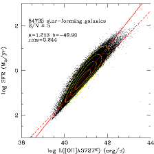
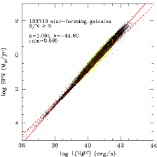
Figure 6: Relation between the SFR (logarithm of M_⊙/yr) and the H$\alpha^{\mathrm{iC}}$ (left), [Oii]^iC (center) or H$\beta^{\mathrm{iC}}$ emission lines luminosities (logarithm of erg/s) for star-forming galaxies in the SDSS DR4 data. The solid line is a least-square fit to the data (errors on $x$ and $y$). These data have been corrected using the unbiased CL01 estimate of dust attenuation. The dashed lines show the previous calibrations obtained with dust estimated from the assumption of a constant intrinsic Balmer ratio (see Fig. 3). Isodensity contours are overplotted in white.

We provide new calibrations to be used on data corrected with a good estimate of the dust attenuation, i.e. not biased towards metallicity. To this end, we corrected the emission-line luminosities using the dust attenuation estimated with the CL01 method, instead of the one estimated from the Balmer decrement. We emphasize that this work is mainly done for comparison purposes: using the CL01 method to estimate the dust attenuation makes our SFR calibration useless since the CL01 SFR is already better constrained.

Fig. 6 shows the relations between the SFR and H$\alpha^{\mathrm{iC}}$, [Oii]^iC or H$\beta^{\mathrm{iC}}$ emission lines. In the three cases, we find as expected an exponent of the power law greater than $1$. However we see that the metallicity dependence of the efficiency factor has not a strong effect on the slope for the H$\alpha^{\mathrm{iC}}$ and H$\beta^{\mathrm{iC}}$ calibrations. We remind the reader that, in contrary to what we have said in Sect. 3.2, the calibrations based on H$\alpha^{\mathrm{iC}}$ or H$\beta^{\mathrm{iC}}$ lines are now slightly different since the ratio between these two lines is not any more assumed constant. We obtain the following results:

$$\left\{\begin{array}[]{ccl}\log\eta_{\mathrm{H}\alpha}^{\mathrm{iC}}&=&44.22\pm 0.03\\ \epsilon_{\mathrm{H}\alpha}^{\mathrm{iC}}&=&1.072\pm 0.001\end{array}\right.$$ (12)

$$\left\{\begin{array}[]{ccl}\log\eta_{[\mathrm{O}\mathsc{ii}]}^{\mathrm{iC}}&=&49.90\pm 0.9\\ \epsilon_{[\mathrm{O}\mathsc{ii}]}^{\mathrm{iC}}&=&1.213\pm 0.03\end{array}\right.$$ (13)

$$\left\{\begin{array}[]{ccl}\log\eta_{\mathrm{H}\beta}^{\mathrm{iC}}&=&44.60\pm 0.03\\ \epsilon_{\mathrm{H}\beta}^{\mathrm{iC}}&=&1.094\pm 0.001\end{array}\right.$$ (14)

In the three cases, the dispersion is reduced thanks to the better estimate of the dust attenuation provided by the CL01 method. Is it now $<0.1$ dex in the H$\alpha^{\mathrm{iC}}$ and H$\beta^{\mathrm{iC}}$ calibrations and $0.24$ dex in the [Oii]^iC calibration.

3.3.2 Dust estimated from SED fitting

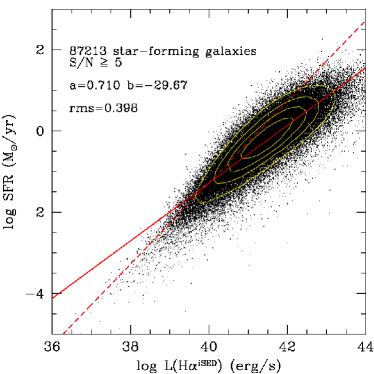
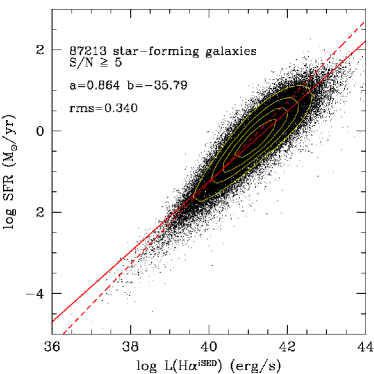
Figure 7: Relation between the SFR (logarithm of M_⊙/yr) and the H$\alpha^{\mathrm{iSED}}$ emission lines luminosity (logarithm of erg/s) for star-forming galaxies in the SDSS DR4 data. The solid line is a least-square fit to the data (errors on $x$ and $y$). The data has been corrected for dust attenuation estimated with the SED fitting method (see Eq. 4). The stellar-to-gas attenuation ratio has been assumed to $0.3$ (left: SDSS mean value), or $0.44$ (right: Calzetti, 2001). The dashed line is the Kennicutt (1998) calibration corrected to our assumed IMF. Isodensity contours are overplotted in white.

One may ask if emission lines can also be used to derived SFR with an estimation of dust attenuation coming from SED fitting. Fig. 7 (left) shows the correlation between the intrinsic H$\alpha$ emission-line luminosity and the SFR in SDSS DR4 data, if we correct H$\alpha$ luminosities with the dust attenuation computed from SED fitting by Kauffmann et al. (2003b) (see Eq. 4). Note that only the $87\,213$ galaxies with an available estimate of the dust attenuation are plotted.

We use a stellar-to-gas attenuation ratio of $0.3$ which corresponds to the mean value observed in the SDSS data (Brinchmann, private communication). We see that the exponent of the power law is quite smaller ($0.710\pm 0.001$), telling us that the SED fitting dust attenuation is even more overestimated at higher masses than with the Balmer decrement method.

But no strong conclusion can be drawn: the dispersion that we find ($0.40$ dex) is indeed quite high and moreover, it does not take into account the likely variations of the stellar-to-gas attenuation ratio between the SDSS data and any other sample. Using instead a stellar-to-gas attenuation ratio of $0.44$ (Calzetti, 2001), we found in Fig. 7 (right) an exponent of the power law of $0.864\pm 0.001$. The derived efficiency factors with a mean stellar-to-gas attenuation ratio of $0.3$ and $0.44$ are respectively $29.67\pm 0.02$ and $35.79\pm 0.03$. We emphasize that a stellar-to-gas attenuation ratio of $0.44$ is not the right value representing these data, even if it gives by chance a less dispersed calibration ($0.34$ dex).

We conclude that the most critical issue in using dust estimated from SED fitting, in order to correct emission lines, comes from the uncertainty in the stellar-to-gas attenuation ratio. This problem makes SFR derived using this method almost completely random on a galaxy per galaxy basis. We note that this method might be used in a statistical way, but with great uncertainties coming both from the dispersion observed in Fig. 7, and from the fact that one has to know the right stellar-to-gas attenuation ratio to apply to his data.

4 SFR calibration without a dust estimate

We present in this section emission-line calibrations of the SFR based on data not corrected for dust attenuation. Because of the small wavelength coverage of many spectroscopic surveys, it is common that not all emission lines necessary to derive a correction for dust attenuation, and to compute a SFR, are present in a given spectrum.

There are two ways to handle such data: (i) use an assumed mean extinction and apply a statistical correction for dust attenuation (see Sect. 4.1); or (ii) use a SFR calibration which provides, still in a statistical approach, a self-consistent correction for dust-attenuation, i.e. with dust properties recovered from another parameter (see Sect. 4.2). We remark that such self-consistent correction depends on the properties of the sample used to do the calibration. Thus, we present in Sect. 4.3 a way to correct for this bias.

4.1 Use of an assumed mean correction

When dust attenuation cannot be reliably derived from the data, it is common in the literature to use an assumed mean correction (frequently $A_{V}=1$).

4.1.1 Standard calibrations with $A_{V}=1$

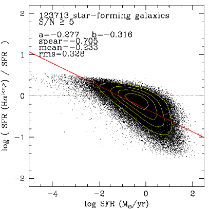
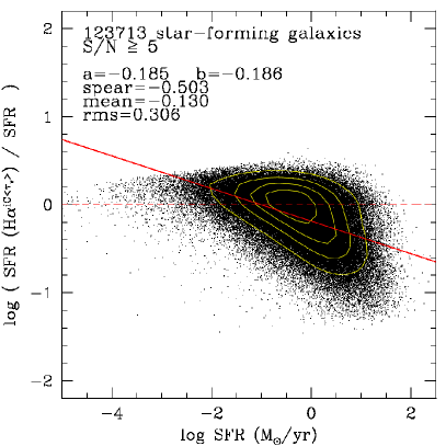
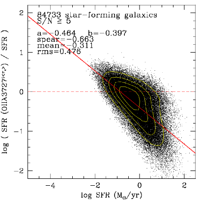
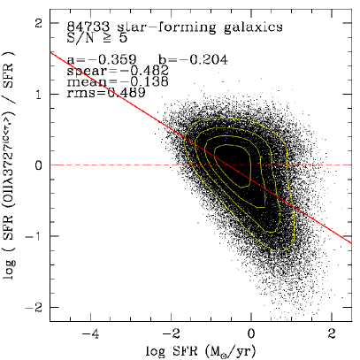
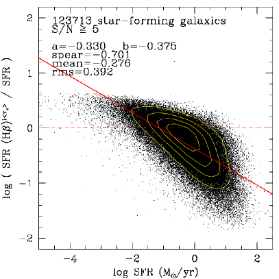
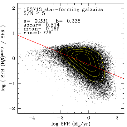
Figure 8: Same legend as in Fig. 2. The studied calibrations are the standard H$\alpha^{\mathrm{i}}$ (top-left), [Oii]ⁱ (middle-left), and H$\beta^{\mathrm{i}}$ (bottom-left) calibrations, or the metallicity-unbiased H$\alpha^{\mathrm{iC}}$ (top-right), [Oii]^iC (middle-right), and H$\beta^{\mathrm{iC}}$ (bottom-right) calibrations, all applied on data corrected using an assumed mean dust attenuation $A_{V}=1$.

In this subsection, we discuss the quality of the standard calibrations used on SDSS DR4 with an assumed mean correction for dust of $A_{V}=1$.

One important question we need to answer is: what kind of calibration should we use on data corrected with a mean dust attenuation ? Should we use the standard calibrations derived with the wrong assumption of a constant intrinsic Balmer ratio (Sect. 3.2), or our new calibrations derived with the better CL01 estimates of the dust (Sect. 3.3) ? The answer basically depends on the way the mean dust attenuation have been estimated (is it biased towards the metallicity dependence of the intrinsic Balmer ratio or not ?).

We thus plot the comparison of both calibrations in Fig. 8. The main conclusion we draw from this figure is that the residuals are not only highly dispersed (rms in the range $0.3$-$0.5$ dex depending on the calibration) but also show a clear residual slope in all cases ($-0.2$ to $-0.5$ depending on the calibration). This residual slope is the signature of the correlation between the dust attenuation and the SFR in galaxies. This correlation is obviously not taken into account by the assumption of a constant dust attenuation for the whole sample.

We note that the residual slopes are significant as shown by the Spearman rank correlation coefficients ($-0.5$ to $-0.7$). It is clear also that the residual slopes obtained with the H$\alpha^{\mathrm{iC}}$, [Oii]^iC , and H$\beta^{\mathrm{iC}}$ calibrations, based on the CL01 estimates of the dust, are not only smaller but also less significant (smaller Spearman rank correlation coefficient).

The method of the assumed mean correction thus leads to poor results, either on galaxy-per-galaxy studies (high dispersion) or on statistical studies (non-negligible residual slope). This method applied with the [Oii] line is particularly inadvisable (worst dispersion and steeper residual slope).

4.1.2 Additional sources of biases

Figure 9: Relation between the dust attenuation estimated with the CL01 method or with the Balmer decrement method, for star-forming galaxies in the SDSS DR4 data. The dashed line is the $y=x$ curve. The solid line is the $y=a\cdot x+b$ curve where $a$ and $b$ are the parameters of the least-square fit (errors in $x$ and $y$), as given in the plot. Isodensity contours are overplotted in white.

We now discuss the additional effect of the use of a wrong mean correction. Following Eq. 2 and 6, the bias introduced on the SFR can be computed like that:

$$\log\left(\frac{\mathrm{SFR^{w}}}{\mathrm{SFR}}\right)=\epsilon\times\frac{\tau_{V}^{\mathrm{w}}-\tau_{V}}{\ln(10)}$$ (15)

where $\tau_{V}^{\mathrm{w}}$ is the wrong assumed dust attenuation, and SFR^w is the wrong derived SFR. Below, we investigate three possible sources of bias.

The first bias comes from the assumption of $A_{V}=1$. The sample used in this study actually shows a mean dust attenuation $\left\langle\tau_{V}^{\mathrm{CL01}}\right\rangle=1.21$ (see Sect. 2 and Fig. 1). Converting from opacities to magnitudes, we obtain $\left\langle A_{V}^{\mathrm{CL01}}\right\rangle=\left\langle\tau_{V}^{\mathrm{CL01}}\right\rangle\times 1.086=1.31$. The difference between the assumed $A_{V}=1$ and the actual value in the sample is partly responsible of the non-null means of the residuals observed in Fig. 8: applying Eq. 15, we find a theoretical bias of the order of $-0.15$ dex, which is similar to the observed values for the CL01 calibrations (Fig. 8 right).

The second bias comes from the dispersion in the distribution of dust attenuation. In the SDSS DR4 data, the dispersion on the derived dust attenuation is $0.64$, which means that the mean dust attenuation may not be assumed with a better precision than $\pm 0.64$. Thus it implies a possible systematic shift of the order of $\pm 0.30$ dex. As stated in Sect. 2, the mean dust attenuation is $\left\langle\tau_{V}^{\mathrm{CL01}}\right\rangle=1.10$ instead of $1.21$ when we add the selection on the [Oii] line: this implies a bias of the order of $\pm 0.05$ dex.

Finally, we remind the reader that he has to think carefully of the origin of the assumed mean correction before applying it, i.e. he has to check whether this assumption comes from a dust attenuation derived with a constant Balmer decrement, or from an unbiased estimation. Having checked that, he would be able to apply the right calibrations. Fig. 9 gives for convenience the relation between $\tau_{V}^{\mathrm{Balmer}}$ and the unbiased $\tau_{V}^{\mathrm{CL01}}$ in the SDSS DR4 data. We fit an empirical relation which follows this formula:

$$\tau_{V}^{\mathrm{Balmer}}=1.53\times\tau_{V}^{\mathrm{CL01}}-0.3$$ (16)

This implies a theoretical bias of the order of $-0.25$ dex, which is again similar to the observed values for the standard calibrations (Fig. 8 left).

Hence we conclude that the use of an assumed mean correction has to be handled with great care.

4.2 Use of a self-consistent correction

As stated in previous subsection, the use of an assumed mean correction has one main drawback: it does not take into account the variation of the dust attenuation as a function of SFR. We thus discuss in this subsection three possible ways to reduce this bias. The idea common to these three possibilities is that the relation between the dust attenuation and the SFR might be itself recovered from the data, i.e. self-consistently.

We explore the self-consistent corrections obtained either from the observed line luminosities, another parameter like the magnitude, or a combination of two emission lines.

4.2.1 Single-line calibrations

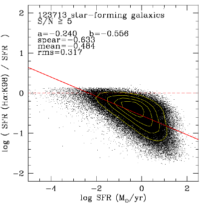
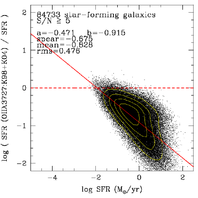
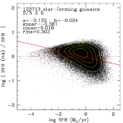
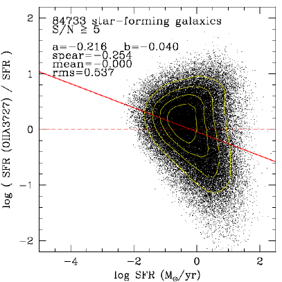
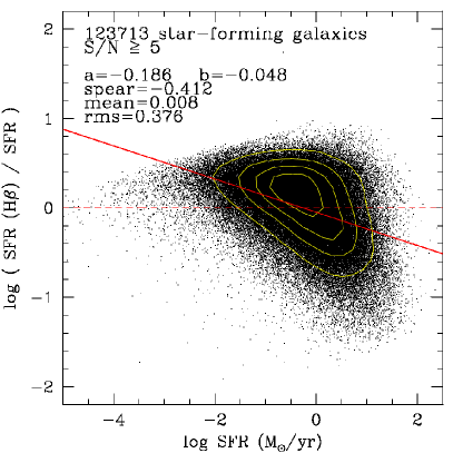
Figure 10: Same legend as in Fig. 2. The studied calibrations are: top-left: Kennicutt (1998) H$\alpha^{\mathrm{i}}$ applied on uncorrected data; top-right: Kennicutt (1998) (corrected by Kewley et al., 2004) [Oii]ⁱ on uncorrected data; middle-left: our new H$\alpha$ calibration; middle-right: our new [Oii] calibration; bottom: our new H$\beta$ calibration.

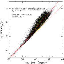
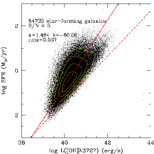
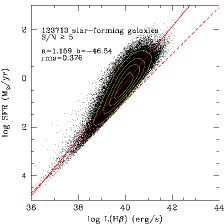
Figure 11: Relation between the SFR (logarithm of M_⊙/yr) and the H$\alpha$ (left), [Oii] (center) or H$\beta$ (right) observed emission lines luminosities (logarithm of erg/s) for star-forming galaxies in the SDSS DR4 data. The solid line is a least-square fit to the data (errors on $x$ and $y$). The dashed lines show the intrinsic calibrations obtained with dust estimated with the Balmer decrement method (see Fig. 3). Isodensity contours are overplotted in white.

The simplest way to apply a self-consistent correction for dust is to relate the dust attenuation to the line luminosity itself. Hence, it consists on calibrating the SFR directly with the observed, not intrinsic, line luminosity with a two-parameter law as described in Eq. 6.

Fig. 10 (top-left) shows the results obtained when using the standard Kennicutt (1992) H$\alpha^{\mathrm{i}}$ calibration on data uncorrected for dust attenuation. We clearly see that the dust attenuation causes an underestimate of the SFR (the mean of the residuals is $-0.48$ dex), and that this effect is increasing with SFR. Moreover the dispersion is $0.32$ dex, and there is a residual slope of $-0.24$ which is significant (Spearman rank correlation coefficient of $-0.63$). Taking this into account, a two parameter law is necessary, differently from what we observed on dust-corrected data in Sect. 3.2.

Fig. 11 (left) shows the correlation between the observed H$\alpha$ emission-line luminosity and the SFR in SDSS DR4 data. We obtain the following new calibration:

$$\left\{\begin{array}[]{ccl}\log\eta_{\mathrm{H}\alpha}&=&46.49\pm 0.04\\ \epsilon_{\mathrm{H}\alpha}&=&1.141\pm 0.001\end{array}\right.$$ (17)

As shown in Fig. 10 (middle-left), the dispersion of this new calibration is $0.30$ dex, which tells us that the SFR recovered without dust attenuation correction are almost twice more dispersed than when an estimate of dust attenuation is available. The mean of the residuals are now almost null ($0.02$ dex). This calibration is better, in terms of the dispersion, than the results obtained with an assumed mean correction (see Sect. 4.1, dispersion of $0.33$ dex) but, it still quite poor.

Unfortunately the use of the two-parameters law, which allows in principle to take into account the dependence between the dust attenuation and the SFR, does not cancel completely the residual slope which is still of $-0.13$. However it is clear, from the comparison of Fig. 8 and Fig. 10 that this remaining residual slope is much less significant (Spearman rank correlation coefficient of $-0.36$ instead of $-0.5$ to $-0.7$).

No estimation of the dust attenuation would be available in most cases where one has to use the [Oii] or the H$\beta$ emission line in order to compute a SFR. This is basically due to the fact the H$\alpha$ line is commonly used to estimate the dust attenuation, and that there is no reason to use another line if the H$\alpha$ line is measured.

Fig. 10 (top-right) shows the results obtained when using the standard Kennicutt (1992) [Oii]ⁱ calibration on data uncorrected for dust attenuation. the dispersion is $0.48$ dex which is high. There is also a significant systematic shift of $-0.83$ dex, plus a significant (Spearman rank correlation coefficient of $-0.68$) residual slope of $-0.47$. Fig. 11 (center) shows the relation between the observed [Oii] emission line luminosity and the SFR in SDSS DR4 data. We obtain the following best-fit values:

$$\left\{\begin{array}[]{ccl}\log\eta_{[\mathrm{O}\mathsc{ii}]}&=&60.06\pm 1.9\\ \epsilon_{[\mathrm{O}\mathsc{ii}]}&=&1.484\pm 0.05\end{array}\right.$$ (18)

But, as we can see from Fig. 10 (middle-right) the dispersion ($0.54$ dex) is higher than the results obtained with an assumed mean correction (see Sect. 4.2, dispersion of $0.48$ dex): the correlation between observed [Oii] luminosity and SFR is rather poor. Nevertheless, this new calibration has the advantage of showing a smaller residual slope of $-0.22$, also much less significant (Spearman rank correlation coefficient of $-0.25$).

Fig. 11 (right) shows the relation between the observed H$\beta$ emission line luminosity and the SFR in SDSS DR4 data, which gives the following parameters:

$$\left\{\begin{array}[]{ccl}\log\eta_{\mathrm{H}\beta}&=&46.54\pm 0.04\\ \epsilon_{\mathrm{H}\beta}&=&1.159\pm 0.001\end{array}\right.$$ (19)

As shown in Fig. 10 (bottom), this new calibration shows a small improvement as compared to the method of an assumed mean correction: dispersion of $0.38$ dex instead of $0.39$ dex, smaller residual slope of $-0.19$, smaller Spearman rank correlation coefficient of $-0.41$ for this residual slope.

The two-parameters calibrations presented in this subsection do not show significant residual slopes as compared to the method of the assumed mean correction. Unfortunately, the gain of having no more significant residual slopes is diminished by the still high dispersion. We claim that these new self-consistent single-line calibrations are however useful when one as no idea of the mean dust attenuation he wants to assume. As stated before, the use of wrong mean correction could lead to a non-negligible systematic bias.

4.2.2 Discussion of previous works

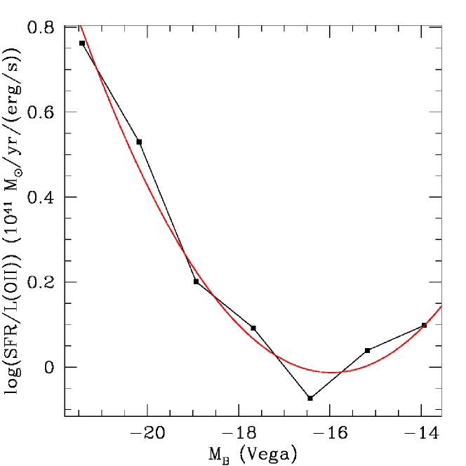
Figure 12: Relation between the SFR efficiency factor of the [Oii] emission line and the $B$-band $k$-corrected absolute magnitude (Vega system). The data points are the values given in Table 2 of Moustakas et al. (2006). The solid curve is our 2nd degree polynomial least square fit with the coefficients given in the text.

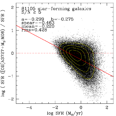
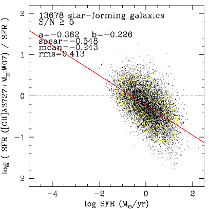
Figure 13: Same legend as in Fig. 2. The studied calibrations are: left: Moustakas et al. (2006) [Oii]+$M_{B}$ calibration; right: Weiner et al. (2007) [Oii]+$M_{H}$ calibration.

Another way to correct self-consistently for dust attenuation, as long as for other parameters (e.g. metallicity, ionization degree, …), is to use the absolute magnitude. Indeed, the absolute magnitude provides an estimate of the dust attenuation through the general correlation between mass and dust attenuation in galaxies. It also provides an estimate of the metallicity through the luminosity-metallicity relation. We note that these calibrations are only derived for the [Oii] line. Again, it is better to correct directly for dust attenuation using the Balmer decrement when H$\alpha$ is observed.

The Moustakas et al. (2006) [Oii] calibration is based on a correction with $B$-band $k$-corrected absolute magnitude, and starts now to be widely used in the literature. However, since the correction is provided by the authors in a few number of discrete points (see Table 2 of their paper), it is not clear how to interpolate between them. The common approach now used in other works is to calculate a global linear regression. Fig. 12 shows that this approach is not valid in the whole domain. We thus provide a parabolic fit which leads to the following final formula:

$$\log\mathrm{SFR}=\log L(\mathrm{[O}\mathsc{ii}\mathrm{]})-41+6.86+0.862\times M_{B}+0.027\times M_{B}^{2}$$ (20)

where $M_{B}$ is the $B$-band $k$-corrected absolute magnitude in the Vega system ($B_{\mathrm{Vega}}=B_{\mathrm{AB}}+0.09$).

Fig. 13 (left) shows how the results obtained with the Moustakas et al. (2006) calibration compares with the reference CL01 SFR. This calibration shows a significant systematic shift of $-0.22$ dex. However, the dispersion of $0.43$ dex is better than previous calibrations on the observed [Oii] luminosity. We observe also a non-negligible residual slope of $-0.30$ (Spearman rank correlation coefficient of $-0.46$), but not stronger than the residual slope obtained with the method of the assumed mean correction.

The Weiner et al. (2007) [Oii] calibration is based on a correction with $H$-band $k$-corrected absolute magnitude. The authors give the slope of the relation between the $\log(\mathrm{[O}\mathsc{ii}\mathrm{]}_{obs}/\mathrm{H}\alpha^{i})$ ratio and the $H$-band $k$-corrected absolute magnitude: $+0.23$ dex/mag. The zero-point is obtained by applying the $0.68$ dex $A(\mathrm{H}\alpha$) extinction to the $\log(\mathrm{[O}\mathsc{ii}\mathrm{]}_{obs}/\mathrm{H}\alpha_{obs})$ ratio of $-0.32$ dex at $M_{H}=-21$. The final formula is:

$$\log\mathrm{SFR}=\epsilon_{\mathrm{H}\alpha}^{\mathrm{i}}\left(\log L(\mathrm{[O}\mathsc{ii}\mathrm{]})-0.23\times M_{H}-3.83\right)-\log\eta_{\mathrm{H}\alpha}^{\mathrm{i}}$$ (21)

where $M_{H}$ is the $H$-band $k$-corrected absolute magnitude in the AB system.

Fig. 13 (right) shows how the results obtained with the Weiner et al. (2007) calibration compares with the reference CL01 SFR. The mean of the residuals is $-0.24$ dex, the dispersion of $0.41$ dex is better than the calibration on the observed [Oii] luminosity, but is still significantly high. Moreover, this smaller dispersion may be only due to the small number of galaxies ($13\,678$) with an available measurement of $M_{H}$ in our sample. Finally, their is also a significant residual slope in this calibration of $-0.36$ (Spearman rank correlation coefficient of $-0.55$).

We conclude that the calibrations proposed by Moustakas et al. (2006) and Weiner et al. (2007) lead to poor results on the SDSS DR4 data. They do neither significantly better, nor significantly worse, than the results obtained with the method of the assumed mean correction, or with our direct calibrations between the SFR and observed line luminosities.

4.2.3 Two-lines calibrations

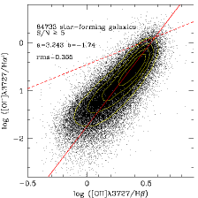
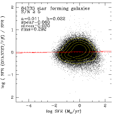
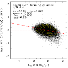
Figure 14: Left: Relation between the [Oii]/H$\alpha^{\mathrm{i}}$ (observed-to-intrinsic) and the [Oii]/H$\beta$ (observed-to-observed) line ratios for star-forming galaxies in the SDSS DR4 data. The solid line is a least-square fit to the data (errors on $x$ and $y$). The dashed line is the $\mathrm{H}\alpha=2.85\cdot\mathrm{H}\beta$ line. Isodensity contours are overplotted in white. Center and right: Same legend as in Fig. 2. The studied calibration are the new [Oii]/H$\beta$ calibrations (center: Eq. 23, right: Eq. ).

Finally we consider the general case where no estimation of the dust attenuation is available. Moustakas et al. (2006) and Weiner et al. (2007) have produced calibrations of the [Oii]/H$\alpha^{\mathrm{i}}$ line ratio against respectively $B$-band or $H$-band absolute magnitudes. Following our idea of using only emission-line measurements, we explore a possible correlation between [Oii]/H$\alpha^{\mathrm{i}}$ (observed-to-intrinsic) and [Oii]/H$\beta$ (observed-to-observed) line ratios. Fig. 14 (left) shows the best-fit relation, as defined by the following equation:

$$\begin{array}[]{cl}\log\left([\mathrm{O}\mathsc{ii}]/\mathrm{H}\alpha^{\mathrm{i}}\right)=&3.243(\pm 0.3)\cdot\log\left([\mathrm{O}\mathsc{ii}]/\mathrm{H}\beta\right)-1.74(\pm 0.09)\end{array}$$ (22)

The mean and the rms of the residuals around the fitted line are respectively $-6\cdot 10^{-10}$ dex and $0.37$ dex. We note that the objects plotted upward the dashed line in Fig. 14 (left) have negative dust attenuation when we derive them from H$\alpha$/H$\beta$ ratio with the assumption of a constant intrinsic Balmer ratio.

Putting Eqs. 9 and 22 together, we obtain the following calibration formula:

$$\log\mathrm{SFR}=\epsilon_{\mathrm{H}\alpha}^{\mathrm{i}}\left(\log L(\mathrm{[O}\mathsc{ii}\mathrm{]})-3.243\cdot\log\left([\mathrm{O}\mathsc{ii}]/\mathrm{H}\beta\right)+1.74\right)-\log\eta_{\mathrm{H}\alpha}^{\mathrm{i}}$$ (23)

Fig. 14 (center) shows the quality of the recovered SFR as compared to the reference CL01 SFR. We see that our new calibration show no significant systematic shift ($0.02$ dex), and no significant residual slope ($0.01$ with a Spearman rank correlation coefficient of $0.06$). Moreover our new calibration shows a dispersion of $0.29$ dex which, while being still higher than the results obtained with a correction for dust attenuation, is the best result obtained in Sect. 4 between all other possibilities: assumed mean dust correction, direct calibration with observed line luminosities, or self-consistent correction with the absolute magnitude.

We also explore the results obtained by doing a direct least-square fit of the SFR as a function of the [Oii] line luminosity and the [Oii]/H$\beta$ line ratio, without assuming the underlying H$\alpha^{\mathrm{i}}$ calibration. We find the following second-degree best-fit relation:

$$\begin{array}[]{r}\log\mathrm{SFR}=-39.21+0.982\cdot\log L(\mathrm{[O}\mathsc{ii}\mathrm{]})-2.396\cdot\log\left([\mathrm{O}\mathsc{ii}]/\mathrm{H}\beta\right)\\ -0.3354\cdot\log\left([\mathrm{O}\mathsc{ii}]/\mathrm{H}\beta\right)^{2}\end{array}$$ (24)

Fig. 14 (right) shows the quality of this other calibration as compared to the reference CL01 SFR. As compared to Eq. 23, the SFR derived with Eq. 24 show a null systematic shift and a smaller dispersion of $0.23$ dex. Nevertheless this smaller dispersion is diminished by a residual slope of $-0.12$ (Spearman rank correlation coefficient of $-0.31$).

Because it is much easier to use and gives better results, our calibrations based on only two observed line fluxes ([Oii] and H$\beta$) should be preferred in most cases with no available correction for dust attenuation. The minimum uncertainty when dealing with data not corrected for dust attenuation is then only $0.23$ dex. We discuss in the following section the different cases where it is better to use Eq. 23 or Eq. 24.

4.3 The self-consistent correction on samples with different properties

It is clear at this stage of our study that all the calibrations derived or studied in Sect. 4 (including those by Moustakas et al., 2006 and Weiner et al., 2007), which are based on observed quantities, depend on the properties of the reference sample. Nevertheless, we emphasize that such statistically significant sample such as the SDSS DR4 data, with a large selection function, is not expected to be strongly biased in favor of one particular population of galaxies.

It might be useful however to know how these calibrations are sensible to the variations of the properties of the studied sample, especially in terms of dust or metallicity.

4.3.1 Dependence on dust

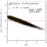
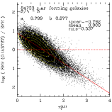
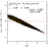
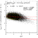
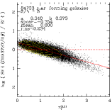
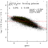
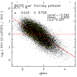
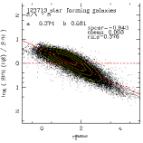
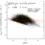
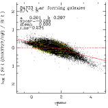
Figure 15: Same legend as in Fig. 2, except that the residuals of the SFR calibration are now plotted as a function of the dust attenuation estimated with the CL01 method (top) or with the Balmer decrement method (bottom). The studied calibrations are, from left to right: H$\alpha$, [Oii], H$\beta$, [Oii]/H$\beta$ (Eq. 23), and [Oii]/H$\beta$ (Eq. 24). All calibrations are related to observed quantities.

Table 1: Coefficients to be used to correct the SFR derived from an observed calibration, as a function of the dust attenuation following Eq. 25. The coefficients are given for a dust attenuation estimated with the CL01 or the Balmer decrement method.

method	CL01		Balmer
calibration	$a$	$b$	$a$	$b$
H$\alpha$	$-0.45$	$0.56$	$-0.28$	$0.44$
[Oii]	$-0.80$	$0.88$	$-0.51$	$0.75$
H$\beta$	$-0.57$	$0.70$	$-0.37$	$0.58$
[Oii]/H$\beta$ (Eq. 23)	$-0.18$	$0.22$	$-0.082$	$0.14$
[Oii]/H$\beta$ (Eq. 24)	$-0.34$	$0.37$	$-0.20$	$0.30$

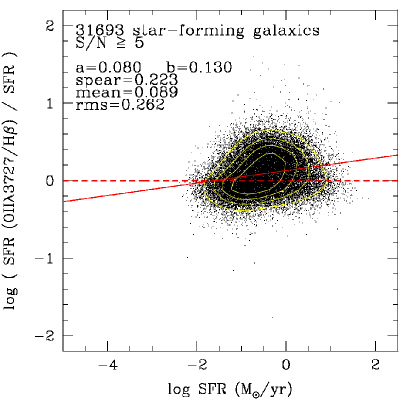
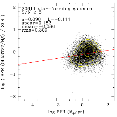
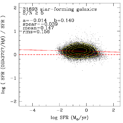
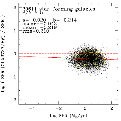
Figure 16: Same legend as in Fig. 2. The studied calibration is the new [Oii]/H$\beta$ calibration given by Eq. 23 (top) or Eq. 24 (bottom), applied on the two dust sub-samples defined in Sect. 2. Left: $\left\langle\tau_{V}^{\mathrm{CL01}}\right\rangle=0.63$, right: $\left\langle\tau_{V}^{\mathrm{CL01}}\right\rangle=1.84$.

We now study in Fig. 15 the residuals of our new calibrations, as compared to the reference CL01 SFR, as a function of the dust attenuation estimated either with the CL01 method, or with the assumption of a constant intrinsic Balmer ratio. This has been done for the poor quality single-line calibrations (H$\alpha$, [Oii], and H$\beta$, see Fig. 10), and for the better quality [Oii]/ H$\beta$ calibration (see Fig. 14 center and right).

In all cases, the means of the residuals are very low, which is expected as we always derived the best-fit calibration.

For the single-line calibrations, we obtain very significant correlations between the residuals and the dust attenuation, with Spearman rank correlation coefficients of the order of $-0.75$ to $-0.95$. Thus, we can derive linear relations which may be used to correct these calibrations for a desired studied sample, for which one has a rough estimate of the mean dust attenuation. The corrective formula as derived from Fig. 15 is:

$$\log\left(\mathrm{SFR}^{\mathrm{corr}}\right)=\log\left(\mathrm{SFR}\right)+a\times\tau_{V}+b$$ (25)

The $a$ and $b$ coefficients are summarized in Table 1. We note that this correction formula give a null correction for a dust attenuation equal to the mean value in the SDSS DR4 sample: $\tau_{V}^{\mathrm{CL01}}=1.21$ in the H$\alpha$ and H$\beta$ cases, and for $\tau_{V}^{\mathrm{CL01}}=1.1$ in the [Oii] case.

For the [Oii]/H$\beta$ two-lines calibration given in Eq. 23, we see that the residuals do not show any more any strong significant correlation with the dust attenuation: smaller slopes, and smaller Spearman rank correlation coefficients of the order of $-0.1$ to $-0.3$. This result shows that the [Oii]/H$\beta$ calibration given in Eq. 23 is not significantly sensitive to variations in the dust attenuation. This calibration can thus reliably been used in any sample without applying a correction. This conclusion is not true for the [Oii]/H$\beta$ calibration given in Eq. 24 which shows similar, but lower, residual slopes as compared to single-line calibrations.

Fig. 16 shows the [Oii]/H$\beta$ calibrations applied on the two sub-samples defined in Sect. 2, with two different dust properties: $\left\langle\tau_{V}^{\mathrm{CL01}}\right\rangle=0.63$ and $\left\langle\tau_{V}^{\mathrm{CL01}}\right\rangle=1.84$. It confirms that the calibration defined in Eq. 23 is reliable when applied on samples with different dust properties: the dispersion does not significantly changes, and the observed residual slopes are not significant (Spearman rank correlation coefficients of the order of $0.2$). In both cases, the observed systematic shifts are in agreement with the correction formula given in Eq. 25 and the coefficients given in Table 1.

4.3.2 Dependence on metallicity

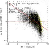
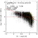
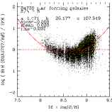
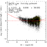
Figure 17: Same legend as in Fig. 2, except that the residuals of the SFR calibration are now plotted as a function of the gas-phase oxygen abundance estimated with the CL01 method. The studied calibrations are, from left to right: H$\alpha$, [Oii], H$\beta$, [Oii]/H$\beta$ (Eq. 23), and [Oii]/H$\beta$ (Eq. 24). All calibrations are related to observed quantities.

Table 2: Coefficients to be used to correct the SFR derived from an observed calibration, as a function of the gas-phase oxygen abundance following Eq. . (first three calibrations) or Eq.  (two last calibrations).

calibration	$a$	$b$	$c$
H$\alpha$	$-0.53$	$4.80$
[Oii]	$-1.50$	$13.35$
H$\beta$	$-0.74$	$6.67$
[Oii]/H$\beta$ (Eq. 23)	$1.47$	$-25.18$	$107.5$
[Oii]/H$\beta$ (Eq. 24)	$0.51$	$-8.96$	$39.3$

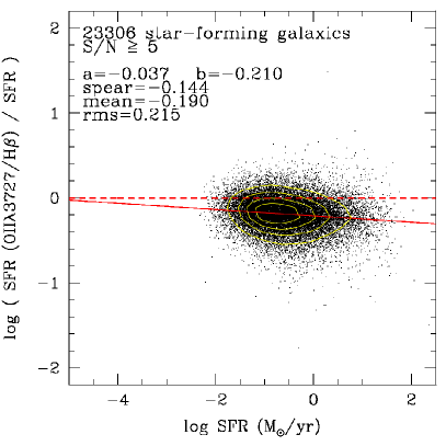
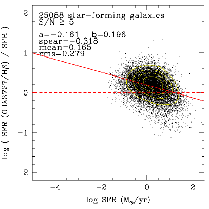
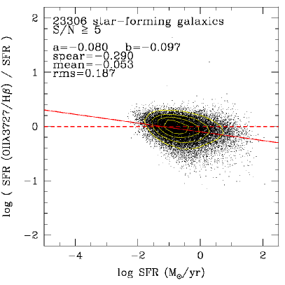
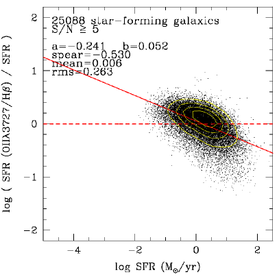
Figure 18: Same legend as in Fig. 2. The studied calibration is the new [Oii]/H$\beta$ calibration given by Eq. 23 (top) or Eq. 24 (bottom), applied on the two metallicity sub-samples defined in Sect. 2. Left: $\left\langle 12+\log(\mathrm{O/H})\right\rangle=8.68$, right: $\left\langle 12+\log(\mathrm{O/H})\right\rangle=9.07$.

We also study the residuals of our new calibrations, as compared to the reference CL01 SFR, as a function of the gas-phase oxygen abundance estimated with the CL01 method. For the single-line calibrations, Fig. 17 shows a significant correlation between these two quantities with Spearman rank correlation coefficients of the order of $-0.5$ to $-0.6$. Thus, we can derive linear relations which may be used to correct these calibrations for a desired studied sample, for which one has a rough estimate of the mean metallicity. The corrective formula as derived from Fig. 17 is:

$$\log\left(\mathrm{SFR}^{\mathrm{corr}}\right)=\log\left(\mathrm{SFR}\right)+a\times x+b$$ (26)

with $x=12+\log(\mathrm{O/H})$. The $a$ and $b$ coefficients are summarized in Table 2. We note that this correction formula give an approximately null correction for a metallicity equal to the mean value in the SDSS DR4 sample: $12+\log(\mathrm{O/H})=8.89$.

For both [Oii]/H$\beta$ calibrations, we have fitted a second degree curve to the residual, which leads to the following corrective formula:

$$\log\left(\mathrm{SFR}^{\mathrm{corr}}\right)=\log\left(\mathrm{SFR}\right)+a\times x^{2}+b\times x+c$$ (27)

with $x=12+\log(\mathrm{O/H})$. The $a$,$b$ and $c$ coefficients are summarized in Table 2.

For the [Oii]/H$\beta$ two-lines calibration given in Eq. 24, we see that the residuals do not show any more any strong significant correlation with the metallicity, with a Spearman rank correlation coefficients of $0.08$. This result shows that the [Oii]/H$\beta$ calibration given in Eq. 24 is not significantly sensitive to variations in the metallicity. This conclusion is not true for the [Oii]/H$\beta$ calibration given in Eq. 23 which shows a Spearman correlation coefficient of $0.57$.

Fig. 18 shows the [Oii]/H$\beta$ calibrations applied on the two sub-samples defined in Sect. 2, with two different metallicity properties: $\left\langle 12+\log(\mathrm{O/H})\right\rangle=8.68$ and $\left\langle 12+\log(\mathrm{O/H})\right\rangle=9.07$. It confirms that the calibration defined in Eq. 24 is reliable when applied on samples with different dust properties: the dispersion does not significantly changes. In both cases, the observed systematic shifts are in agreement with the correction formula given in Eq. 27 and the coefficients given in Table 2.

We conclude that:

• The [Oii]/H$\beta$ calibration given in Eq. 23 is weakly sensitive to variations in dust attenuation. It can be applied on samples with an assumed metallicity, using the corrective formula given in Eq. 27.

• The [Oii]/H$\beta$ calibration given in Eq. 24 is not sensitive to variations in metallicity. It can be applied on samples with an assumed dust attenuation, using the corrective formula given in Eq. 25.

5 Conclusions

We draw the following conclusions from our study:

• As already shown in many previous studies, we confirm from SDSS DR4 data the the best emission-line calibration of the SFR is based on H$\alpha^{\mathrm{i}}$, this one being corrected for dust attenuation (see Sect. 3.2.1). This calibration has an uncertainty of $0.17$ dex.

• If the dust has been estimated from the wrong assumption of a constant intrinsic Balmer ratio, the standard one-parameter Kennicutt (1998) scaling law gives good enough results. Nevertheless, the SDSS DR4 data has shown a $-0.11$ dex systematic shift which can be corrected either by applying a mean shift in the opposite direction, or by using a two-parameter power law (see Fig. 2, Fig. 3 and Eq. 7).

• When H$\alpha^{\mathrm{i}}$ is not observed but a correction for dust attenuation is still available, the Kennicutt (1998) law based on [Oii]ⁱ (and corrected for dust by Kewley et al., 2004) gives good results but shows a higher dispersion (see Fig. 2).

• This dispersion may be reduced by taking into account the dependence of [Oii]ⁱ on the metallicity. However, the metallicity correction proposed by Kewley et al. (2004) does not end to a significant improvement, while it relies on a very uncertain calibration of the metallicity, as shown by Kewley & Ellison (2008) (see Fig. 4 and Fig. 5).

• A very good correction of this effect is rather obtained by using the [Oii]ⁱ and H$\beta^{\mathrm{i}}$ lines together or, even better, H$\beta^{\mathrm{i}}$ alone (see Eq. 9, Eq. 10 and Eq. 11).

• We caution the reader against the use of the inadequate SFR calibration when data is corrected for dust estimated from another method (e.g. CL01 method). If the method to derive dust attenuation is not biased towards the wrong assumption of a constant intrinsic Balmer ratio, then a different SFR calibration should be used (see Sect. 3.3.1, Fig. 6, Eq. 12, Eq. 13, and Eq. 14).

• We advise the reader not to use dust estimated from SED fitting in order to calculate SFR from emission lines. This method leads to highly uncertain results because of the high dispersion in the stellar-to-gas attenuation ratio (see Fig. 7). We emphasize that dust attenuation estimated from SED fitting would be reliable only if it is applied to the light emitted by stars, not to emission lines.

• When no estimation of the dust attenuation is available, it is common in the literature to assume a mean correction, typically $A_{V}=1$. We advise the reader to use such method with great care for two reasons: (i) the SFRs recovered with the assumption of a constant dust attenuation are biased by a non-negligible residual slope, coming from the correlation between dust attenuation and SFR (see Sect. 4.1.1 and Fig. 8); (ii) additional biases come from the choice of the assumed dust attenuation which is likely not to be the right one. The choice of a wrong assumed dust attenuation leads to non-negligible systematic shifts (see Sect. 4.1.2).

• We have derived new direct calibrations between the SFR and the observed line luminosities which are still quite poor in terms of dispersion, even if they do not show any more a significant residual slope (see Fig. 10, Fig. 11, Eq. 17, Eq. 18 and Eq. 19).

• The calibrations proposed by Moustakas et al. (2006) or Weiner et al. (2007) which include a correction based on the $B$-band or $H$-band $k$-corrected absolute magnitudes do neither significantly better nor significantly worse (see Fig. 13).

• We derive two new two-lines calibrations based only on the [Oii] and H$\beta$ observed line flux. These calibrations give the best results among all calibrations based on observed quantities (i.e. not reliably corrected for dust attenuation). It shows no systematic shift, no significant residual slope, and a reduced dispersion (see Fig. 14, Eq. 23 and Eq. 24). The minimum uncertainty with data not corrected for dust attenuation is $0.23$ dex.

• We have studied the relation between the residuals of our calibrations based on observed quantities, and the dust attenuation (see Fig. 15). There is a clear correlation for single-line calibrations, which can be corrected (see Eq. 25 and Table 1). We have also found a correlation between the residuals of our calibrations based on observed quantities (see Fig. 17), which can be corrected for single-line calibrations using Eq. 26 and Table 2.

• Among our two new [Oii]/H$\beta$ calibrations, the one defined by Eq. 23 is designed to be used on a sample with an assumed metallicity and an unknown dust attenuation, while the one defined by Eq. 24 give better results on samples with unknown metallicity and an assumed dust attenuation.