Fundamental vibration mode in a highly inhomogeneous star

Abstract

The eigenfrequency problem of fundamental vibration mode in a highly inhomogeneous star modeled by self-gravitating mass of viscous liquid with singular density at the center is considered in juxtaposition with that for Kelvin fundamental mode in the liquid star model with uniform density. Particular attention is given to the difference between spectral equations for the frequency and lifetime of $f$-mode in the singular and homogeneous star models. The newly obtained results are discussed in the context of theoretical asteroseismology of white dwarfs.

1 Introduction

The term fundamental mode has been introduced in the theory of stellar pulsations by Cowling (1941) from hydrodynamical model of a heavy mass of inviscid incompressible liquid of uniform density $\rho$ undergoing free oscillations with nodeless irrotational velocity of fluctuating flow. The extended discussion of the eigenfrequency problem of this model, whose solution is due to Kelvin (1863), can be found elsewhere (e.g. Lamb 1945, Chandrasekhar 1961, Bastrukov 1996). An outstanding importance of this fiducial model for theoretical asteroseismology is that it sets the standard for analytic study of non-radial pulsations of the main-sequence stars (Cox 1980, Unno et al 1989) and serves as an example, according to Chandrasekhar (1961), of ”at least one problem for which analytic solution can be found” and which illustrates ”the type of difficulties one must confront in the other problem”, because ”in most instances, the problems become of such complexity and involve so many parameters that elementary methods of solution seem impracticable”.

The purpose of this work is to explore some peculiarities of the fundamental vibration mode in the inhomogeneous stars. In approaching the topic like this it seems better to start with a brief outline of assumptions lying at the base of the $f$-mode frequency computation in the homogeneous liquid star model in which the uniform equilibrium density is not altered, $\delta\rho=0$. The obvious consequence of this assumption steaming from the continuity equation

$$\delta{\dot{\rho}}=-\nabla\,(\rho\,\delta{\bf v})=-(\delta{\bf v}\cdot\nabla)\,\rho-\rho\,\nabla\cdot\delta{\bf v}$$ (1)

is that the velocity of flow oscillating in a spherical mass of incompressible liquid of uniform density is described by the potential vector field of the form

$$\nabla\cdot\delta{\bf v}({\bf r},t)=0,\quad\delta{\bf v}({\bf r},t)=\nabla\chi({\bf r},t),$$ (2)

$$\nabla^{2}\chi({\bf r},t)=0,\quad\chi({\bf r},t)=A_{\ell}\,r^{\ell}\,P_{\ell}(\cos\theta){\dot{\alpha}}(t).$$ (3)

The last equation exhibits nodeless character of the velocity flow as a function of distance from center to the surface of the star. It is this feature of oscillating flow is regarded as the major kinematic signature of fundamental vibration mode.

In this paper we relax the basic assumption of the homogeneous liquid star model about uniform equilibrium density, preserving the above major kinematic signature of $f$-mode. Specifically, we consider admittedly idealized a highly inhomogeneous liquid star model in which the non-uniform density profile has singularity at the star center of the form

$$\rho(r)=\frac{5}{6}\rho_{s}\left({\frac{R}{r}}\right)^{1/2}.$$ (4)

One of the most conspicuous features of this density profile is that the total mass of such a star

$$M=\int\rho(r)\,d{\cal V}=\frac{4\pi}{3}\rho_{s}R^{3}$$ (5)

is finite and identical to that for the total mass of the canonical homogenous liquid star model. In somewhat different context the model of inhomogeneous liquid star with similar density profile has been briefly discussed by Clayton (1986). This curious feature of the model, which from now on is referred to as the singular star model, is interesting in its own right because it permits too analytically tractable solution of the eigenfrequency problem for $f$-mode. Perhaps the most striking feature distinguishing vibrational behavior of inhomogeneous from homogeneous one is that the nodeless non-rotational vibrations of a spherical liquid mass of non-uniform density are of substantially compressional character, as it follows from the continuity equation. Therefore, one of the prime purposes of our study is to find out how this striking distinction between the density profiles of homogeneous and inhomogeneous models is reflected in the frequency and lifetime spectra of fundamental vibration mode.

The paper is organized as follows. In section 2, a general mathematical treatment of the inhomogeneous star vibrations in the fundamental mode on the basis of the Rayleigh’s energy variational principle is outlined. In section 3, the detailed analytic computation of the spectral equations for the frequency and lifetime of $f$-mode in the singular liquid star model is presented followed by their comparison with those for the Kelvin fundamental mode in homogeneous star model which is the subject of Section 4. The newly obtained results are highlighted in section 5 and briefly discussed in the context of current development of theoretical asteroseismology of white dwarfs.

2 General equations of nodeless stellar vibrations in fundamental mode

The state of motion of flowing stellar matter under the action of forces of buoyancy, gravity and viscous stress is uniquely described in terms of five dynamical variables, to wit, the density $\rho({\bf r},t)$, three components of the flow velocity ${\bf v}({\bf r},t)$ and the pressure $p({\bf r},t)$ obeying the coupled equations of fluid-mechanics and Newtonian universal gravity

$$\frac{d\rho}{dt}=-\rho\,\frac{\partial v_{k}}{\partial x_{k}},\quad\quad\frac{d}{dt}=\frac{\partial}{\partial t}+v_{k}\frac{\partial}{\partial x_{k}},$$ (6)

$$\rho\frac{dv_{i}}{dt}=-\frac{\partial p}{\partial x_{i}}+\rho\frac{\partial U}{\partial x_{i}}+\frac{\partial\pi_{ik}}{\partial x_{k}},$$ (7)

$$\frac{dp}{dt}=\frac{\Gamma_{1}p}{\rho}\frac{d\rho}{dt}=-\Gamma_{1}\,p\frac{\partial v_{k}}{\partial x_{k}},\quad\quad\Gamma_{1}=\frac{\partial\ln p}{\partial\ln\rho},$$ (8)

$$\nabla^{2}U=-4\pi G\rho.$$ (9)

The equation for density $\rho$ is the condition of continuity of flowing stellar matter. The Navier-Stokes equation for the velocity flow expresses the second law of Newtonian dynamics for viscous liquid and equation for pressure is the condition of adiabatic behavior of stellar matter; $\Gamma_{1}$ stands for the adiabatic coefficient of gaseous pressure in the star. This latter condition means that in the process of motion, like vibrations, the time scale of energy exchange between infinitesimally close elementary volume of liquid is much longer than characteristic period of oscillations (e.g. Huang 1987, Kawaler & Hansen 1994). The tensor of Newtonian viscous stresses is given by

$$\pi_{ik}=2\eta\,v_{ik}+\left(\zeta-\frac{2}{3}\,\eta\right)v_{jj}\,\delta_{ik},\quad\quad v_{ik}=\frac{1}{2}\left(\nabla_{k}v_{i}+\nabla_{i}v_{k}\right).$$ (10)

In computing frequency of fundamental vibration mode, the equilibrium density profile $\rho$, the pressure $P_{c}$ at the star center as well as the transport coefficients of stellar matter, the shear $\eta$ and the bulk $\zeta$ viscosities, are regarded as input, in advance given, parameters.

The potential of self-gravity $U(r)$ and pressure $p(r)$ in motionless, ${\bf v}=0$, state of hydrostatic equilibrium, are the solutions of coupled equations

$$\nabla_{i}\,p(r)=\rho(r)\nabla_{i}\,U(r),\quad\quad\nabla^{2}U(r)=-4\pi G\rho(r).$$ (11)

The gravity potential $U$ is determined, in effect, by Poisson equation for internal potential $U_{i}$ and Laplace equation for external one $U_{e}$ supplemented by the standard boundary conditions of the continuity of these potentials and their normal derivatives on the star surface

$$\nabla^{2}U_{i}(r)=-4\pi G\rho(r),\quad r\leq R,\quad\quad\nabla^{2}U_{e}(r)=0,\quad r>R,$$ (12)

$$U_{i}(r)=U_{e}(r)\Big{|}_{r=R},\quad\quad\frac{dU_{i}(r)}{dr}=\frac{dU_{e}(r)}{dr}\Big{|}_{r=R}.$$ (13)

The general solution of equation for pressure is specified by standard boundary condition of stress-free surface $p(r=R)=0$.

The equations of linear oscillations of stellar matter about stationary state of hydrostatic equilibrium of a star with non-uniform equilibrium density, $\rho=\rho(r)$, are obtained by applying to (6)-(9) the standard procedure of linearization

$$\rho\to\rho(r)+\delta\rho({\bf r},t)\,\quad p\to p(r)+\delta p({\bf r},t)$$ (14)

$$v_{i}\to v_{i}+\delta v_{i}({\bf r},t),\quad[v_{i}=0],\quad U\to U({\bf r})+\delta U({\bf r},t).$$ (15)

As was stated, in this work we focus on the regime of irrotational vibrations in which the velocity field of fluctuating flow subjects to

$$\nabla\cdot\delta{\bf v}=0,\quad\nabla\times\delta{\bf v}=0.$$ (16)

Given this, the continuity equation takes form

$$\delta{\dot{\rho}}=-(\delta v_{k}\nabla_{k})\rho.$$ (17)

The liner fluctuations of the flow velocity are governed by linearized Navier-Stokes equation

$$\rho\delta{\dot{v}}_{i}=-\nabla_{i}\delta p+\rho\nabla_{i}\delta U+\delta\rho\nabla_{i}U+\nabla_{k}\delta\pi_{ik},$$ (18)

$$\delta\pi_{ik}=2\eta\delta v_{ik},\quad\quad\delta v_{ik}=\frac{1}{2}(\nabla_{i}\delta v_{k}+\nabla_{k}\delta v_{i}).$$ (19)

From (8) it follows that rate of change in the pressure is controlled by equation

$$\delta{\dot{p}}=-(v_{k}\nabla_{k})\,p.$$ (20)

Fluctuations in potential of self-gravity inside the star $\delta U=\delta U_{i}$, caused by fluctuations in density $\delta\rho$, subject to the Poisson equation

$$\nabla^{2}\delta U=-4\pi G\,\delta\rho.$$ (21)

The energy balance in the process of oscillations is controlled by equation

$$\frac{\partial}{\partial t}\int\frac{\rho\delta v^{2}}{2}\,d{\cal V}=-\int[(\delta v_{k}\nabla_{k})\delta p-\rho(\delta v_{k}\nabla_{k})\delta U-\delta\rho(\delta v_{k}\nabla_{k})U-\delta\pi_{ik}\delta v_{ik}]\,d{\cal V}$$ (22)

which is obtained after scalar multiplication of (18) by $\delta v_{i}$ and integration over the star volume. To compute the eigenfrequency of vibrations we take advantage of the Rayleigh’s energy variational principle at the base of which lies the following separable representation of fluctuating variables

$$\delta v_{i}({\bf r},t)=a_{i}({\bf r}){\dot{\alpha}}(t),\quad\delta U({\bf r},t)=\phi({\bf r}){\alpha}(t),$$ (23)

$$\delta\rho({\bf r},t)=\tilde{\rho}({\bf r})\,{\alpha}(t),\quad\tilde{\rho}({\bf r})=-(a_{k}({\bf r})\nabla_{k})\,\rho(r),$$ (24)

$$\delta p({\bf r},t)=\tilde{p}({\bf r})\,{\alpha}(t),\quad\tilde{p}({\bf r})=-(a_{k}({\bf r})\nabla_{k})\,p(r),$$ (25)

$$\delta\pi_{ik}({\bf r},t)=2\eta\,\delta v_{ik}=2\eta\,a_{ik}({\bf r}){\dot{\alpha}}(t),$$ (26)

$$\delta v_{ik}({\bf r},t)=a_{ik}({\bf r}){\dot{\alpha}}(t),\quad\quad a_{ik}({\bf r})=\frac{1}{2}(\nabla_{i}a_{k}({\bf r}),+\nabla_{k}a_{i}({\bf r})).$$ (27)

Hereafter $a_{i}({\bf r})$ stands for the time-independent field of instantaneous material displacements and $\alpha(t)$ for the temporal amplitude of oscillations. The key idea of such representation is that it transforms equation of energy balance (22) into equation for $\alpha$ having well-familiar form of equation of damped oscillations

$$\frac{d{\cal E}}{dt}=-2{\cal F},\quad\quad{\cal E}=\frac{{\cal M}{\dot{\alpha}}^{2}}{2}+\frac{{\cal K}\alpha^{2}}{2},\quad{\cal F}=\frac{{\cal D}{\dot{\alpha}^{2}}}{2},$$ (28)

$${\cal M}{\ddot{\alpha}}+{\cal D}{\dot{\alpha}}+{\cal K}\alpha=0,$$ (29)

$${\cal M}=\int\rho(r)a_{k}\,a_{k}\,d{\cal V},\quad{\cal D}=2\int\eta(r)a_{ik}\,a_{ik}\,d{\cal V}$$ (30)

$${\cal K}=\int[(a_{k}\,\nabla_{k}\,\rho(r))\,(a_{k}\,\nabla_{k}\,U({\bf r}))-\rho(r)(a_{k}\,\nabla_{k})\phi({\bf r})-(a_{k}\nabla_{k})\,(a_{k}\nabla_{k})p(r)]\,d{\cal V}.$$ (31)

Here ${\cal E}$ is the energy of free, non-dissipative, oscillations and ${\cal F}$ is the dissipative function of Rayleigh describing their damping by shear viscosity of stellar matter. The solution of (29) is given by

$$\alpha(t)=\alpha_{0}\,\exp(-t/\tau)\,\cos\omega(\tau)t,$$ (32)

$$\omega^{2}(\tau)=\omega^{2}[1-(\omega\tau)^{-2}],\quad\omega^{2}=\frac{{\cal K}}{{\cal M}},\quad\tau=\frac{2{\cal M}}{{\cal D}}$$ (33)

where $\omega(\tau)$ is the frequency of dissipative oscillations damped by viscosity, $\omega$ is the frequency of free oscillations and $\tau$ is their lifetime. Thus, to compute the frequency and lifetime one need to specify all variables entering integral parameters of inertia ${\cal M}$, stiffness ${\cal K}$ and viscous friction ${\cal D}$.

We start with the field of instantaneous displacements $a_{k}({\bf r})$ which is the key kinematic characteristics of $f$-mode. In the star undergoing irrotational oscillations in the $f$-mode, the shape of an arbitrary spherical surface takes the form of harmonic spheroids which are described by

$$r(t)=r[1+\alpha_{\ell}(t)P_{\ell}(\zeta)],\quad\zeta=\cos\theta$$ (34)

where $P_{\ell}(\zeta)$ is the Legendre polynomial of the multipole order $\ell$ specifying the overtone number in fundamental vibration mode. In the system with fixed polar axis the potential field of velocity is found from Laplace equation supplemented by boundary condition that radial component of velocity on the star surface equals to the rate of the surface distortions taking the shape of harmonic spheroids

$$\nabla_{k}\,\delta v_{k}=0,\quad\delta v_{k}=\nabla_{k}\chi,\quad\nabla^{2}\chi=0\quad\to\quad\chi=A_{\ell}\,r^{\ell}\,P_{\ell}(\zeta)\,{\dot{\alpha}}(t),$$ (35)

$$\delta v_{r}\big{|}_{r=R}={\dot{R}}(t),\quad R(t)=R[1+\alpha_{\ell}(t)P_{\ell}(\zeta)].$$ (36)

Taking into account that $\delta{\bf v}({\bf r},t)={\bf a}({\bf r}){\dot{\alpha}}(t)$ one has

$${\bf a}({\bf r})=A_{\ell}\nabla r^{\ell}\,P_{\ell}(\zeta),\quad\quad A_{\ell}=\frac{1}{\ell R^{\ell-2}}.$$ (37)

In terms of this field, the linearized equations for the density $\delta\rho$ and for the pressure $\delta p$ reads

$$\delta\rho({\bf r},t)=\tilde{\rho}({\bf r})\,{\alpha}(t),\quad\tilde{\rho}({\bf r})=-({\bf a}\cdot\nabla)\,\rho(r)=-A_{\ell}P_{\ell}(\zeta)\ell\,r^{\ell-1}\frac{\partial\rho(r)}{\partial r},$$ (38)

$$\delta p({\bf r},t)=\tilde{p}({\bf r})\,{\alpha}(t),\quad\tilde{p}({\bf r})=-({\bf a}\cdot\nabla)\,p(r)=-A_{\ell}P_{\ell}(\zeta)\ell\,r^{\ell-1}\frac{\partial p(r)}{\partial r}$$ (39)

where $\rho(r)$ and $p(r)$ are the density and pressure of gravitationally equilibrium, hydrostatic, configuration.

To compute variations in the potential of gravity one must consider two equations for internal $\delta U_{i}$ and external $\delta U_{i}$ potentials

$$\nabla^{2}\delta U_{i}({\bf r},t)=-4\pi\,G\delta\rho({\bf r},t),\quad\nabla^{2}\phi_{i}({\bf r})=-4\pi\,G\tilde{\rho}({\bf r})$$ (40)

$$\nabla^{2}\delta U_{e}({\bf r},t)=0,\quad\nabla^{2}\phi_{e}({\bf r})=0.$$ (41)

The outlined energy variational method provides a general framework for computing the frequency of $f$-mode in a inhomogeneous Newtonian liquid star with arbitrary form of non-uniform density profile.

3 The singular star model

As was stated, we use the term singular star for a self-gravitating mass of viscous liquid with the non-uniform and singular in the star center density profile given by equation (4) whose total mass is identical to that for homogenous star model. For such a singular star, the equilibrium potentials and fields of universal gravity are given by

$$\nabla^{2}U_{i}(r)=-4\pi G\rho(r),\quad\rho(r)=\frac{5}{6}\rho_{s}\left({\frac{R}{r}}\right)^{1/2},\quad M=\int\rho(r)\,d{\cal V}=\frac{4\pi}{3}\rho_{s}R^{3},$$ (42)

$$U_{i}(r<R)=\frac{20\pi}{9}G\rho_{s}R^{2}\left[1-\frac{2}{5}\left(\frac{r}{R}\right)^{3/2}\right]=\frac{5}{3}\frac{GM}{R}\left[1-\frac{2}{5}\left(\frac{r}{R}\right)^{3/2}\right],$$ (43)

$${\rm\bf g}_{i}(r<R)=-\nabla U_{i}=\frac{GM}{R^{3}}\left(\frac{r}{R}\right)^{1/2}{\bf r},$$

$$U_{e}(r>R)=\frac{4\pi}{3}G\rho_{s}\frac{R^{3}}{r}=\frac{GM}{r},\quad{\rm\bf g}_{e}(r>R)=-\nabla U_{e}=\frac{GM}{r^{3}}{\bf r}.$$ (44)

The hydrostatic pressure obeying the boundary condition of free surface $p(r)|_{r=R}=0$ reads

$$p(r)=\frac{10\pi}{9}G\rho_{s}^{2}R\left(R-r\right)=P_{c}\left(1-\frac{r}{R}\right),\quad P_{c}=\frac{10\pi}{9}G\rho_{s}^{2}R^{2}=\frac{5}{8\pi}\frac{GM^{2}}{R^{4}}.$$ (45)

It is remarkable that the pressure at the star center, where the density has singularity, is finite and its radial profile is linear function of distance from the center to the star surface. The pressure in the center is defined by equation of state of the stellar matter.. With in advance given equation of state for $P_{c}$ the rightmost identity in (45) is considered as definition of the star radius. The internal gravitational energy is

$$W_{s}=\frac{1}{2}\int\rho_{s}\,U_{i}d{\cal V}=\frac{11}{18}\frac{GM^{2}}{R}\simeq 1.02W,\quad W=\frac{3}{5}\frac{GM^{2}}{R}$$ (46)

where $W$ is the total gravitational energy of homogeneous star of equivalent mass $M$. To take into account the compression effect of self-gravity on mechanical property of star matter we adopt the suggestion of work (Bastrukov et al 2007a) that radial profile of viscosity coefficient is identical to that for the equilibrium pressure profile, that is, of the form

$$\nu(r)=\nu_{c}\left(1-\frac{r}{R}\right)$$ (47)

where $\nu_{c}$ is the shear viscosity in the star center which along with $\rho_{s}$ and $P_{c}$ are regarded as input parameters of the model.

3.1 Exact solution of Poisson equation for variations of self-gravity potential in singular star

Having defined the equilibrium profiles of density $\rho(r)$, the pressure $p(r)$, the shear viscosity profile $\nu(r)$ and knowing the field of instantaneous displacements ${\bf a}({\bf r})$ we are able to compute the inertia ${\cal M}$ and viscous friction ${\cal D}$. However, in order to compute the stiffness ${\cal K}$ we must calculate fluctuations in the potential of self-gravity $\delta U({\bf r},t)=\phi({\bf r})\alpha(t)$, that is, to solve Poisson equation for $\phi({\bf r})$ with a fairly non-trivial right part

$$\nabla^{2}\phi_{i}(r,\zeta)=-\frac{5\pi}{3}A_{\ell}\,G\rho_{s}\,R^{1/2}\,\ell\,r^{\ell-5/2}P_{\ell}(\zeta).$$ (48)

In the spherical polar coordinates we have

$$\frac{1}{r^{2}}\frac{\partial}{\partial r}r^{2}\frac{\partial\phi_{i}(r,\theta)}{\partial r}+\frac{1}{r^{2}\sin\theta}\frac{\partial}{\partial\theta}\sin\theta\frac{\partial\phi_{i}(r,\theta)}{\partial\theta}=-\frac{5\pi}{3}\,A_{\ell}\,G\rho_{s}\,R^{1/2}\,\ell\,r^{\ell-5/2}P_{\ell}(\cos\theta).$$ (49)

Assuming a solution of the form

$$\phi_{i}(r,\theta)=\frac{u(r)}{r}\,P_{\ell}(\cos\theta)$$ (50)

and taking into account that $P_{\ell}(\cos\theta)$ is the solution of equation

$$\frac{1}{\sin\theta}\frac{\partial}{\partial\theta}\sin\theta\frac{\partial P_{\ell}(\cos\theta)}{\partial\theta}=-\ell(\ell+1)\,P_{\ell}(\cos\theta)$$ (51)

we obtain

$$r^{2}\frac{\partial^{2}u(r)}{\partial r^{2}}-\ell(\ell+1)u(r)=-\frac{5\pi}{3}\,A_{\ell}\,G\rho_{s}\,R^{1/2}\,\ell\,r^{\ell+1/2}.$$ (52)

The general solution of equation for $\phi_{i}$, which is finite at the origin, is given by

$$\phi_{i}(r,\theta)=\left\{C\,r^{\ell}+\frac{20\pi}{3}\frac{\ell}{4\ell+1}\,\,A_{\ell}\,\rho_{s}\,G\,R^{1/2}r^{\ell-1/2}\right\}P_{\ell}(\cos\theta)$$ (53)

Outside the star we have

$$\nabla^{2}\delta U_{e}=0\quad\to\quad\nabla^{2}\phi_{e}({\bf r})=0,$$ (54)

$$\phi_{e}=D\,r^{-\ell-1}P_{\ell}(\cos\theta).$$ (55)

The arbitrary constants $C$ and $D$ are eliminated from boundary conditions

$$\phi_{i}=\phi_{e}\Big{|}_{r=R},\quad\quad\frac{\partial\phi_{i}}{\partial r}=\frac{\partial\phi_{e}}{\partial r}\Big{|}_{r=R}.$$ (56)

which yield

$$C=-\frac{10\pi}{3}\,A_{\ell}\,\rho_{s}\,G\,\frac{\ell}{2\ell+1},\quad D=\frac{10\pi}{3}\,A_{\ell}\,\rho_{s}\,G\,\frac{\ell}{(4\ell+1)(2\ell+1)}R^{2\ell+1}.$$ (57)

Finally, we obtain

$$\phi_{i}(r,\theta)=-\frac{10\pi}{3}\frac{\ell}{2\ell+1}A_{\ell}\,\rho_{s}\,G\,\left[r^{\ell}-\frac{2(2\ell+1)}{4\ell+1}R^{1/2}\,r^{\ell-1/2}\right]P_{\ell}(\cos\theta).$$ (58)

It is worth emphasizing that following this line of argument one can get the solutions of Poisson equation for a more wide class of inhomogeneous star models undergoing nodeless spheroidal vibrations with non-rotational field of velocity. Also, the method and obtained solution can be useful in the study of electrodynamic problems of astrophysical interest.

3.2 Spectral equations for frequency and lifetime of $f$-mode

The mass parameter ${\cal M}$ is given by

$${\cal M} = \int_{V}\rho(r)\,[a^{2}_{r}+a^{2}_{\theta}]\,d{\cal V}=\frac{5\pi}{3}\rho_{s}A_{\ell}^{2}R^{1/2}\int\limits_{0}^{R}\,r^{2\ell-1/2}\,dr\,\int\limits_{-1}^{+1}\left[\ell^{2}P^{2}_{\ell}(\zeta)+\left(1-\zeta^{2}\right)\left(\frac{dP_{\ell}(\zeta)}{d\zeta}\right)^{2}\right]d\zeta$$ (59)

$$= \frac{20\pi}{3}\,A_{\ell}^{2}\,\rho_{s}\,R^{2\ell+1}\,\frac{\ell}{4\ell+1}.$$

Computation of the viscous friction parameter, with the non-uniform profile of shear viscosity (47), yields

$${\cal D} = 2\int\eta(r)a_{ij}a_{ij}\,d{\cal V}=2\int\eta(r)\left(a_{rr}^{2}+a_{\theta\theta}^{2}+a_{\phi\phi}^{2}+2a_{r\theta}^{2}\right)d{\cal V}$$ (60)

$$= 8\pi A_{\ell}^{2}\int\limits_{0}^{R}\eta(r)r^{2\ell-2}dr\int\limits_{-1}^{1}\left[\ell^{2}(\ell^{2}-\ell+1)P_{\ell}(\zeta)^{2}-\ell(\ell+1)\zeta P_{\ell}(\zeta)\frac{dP_{\ell}(\zeta)}{d\zeta}+\zeta^{2}\left(\frac{dP_{\ell}(\zeta)}{d\zeta}\right)^{2}\right.$$

$$+ \left.(\ell-1)^{2}(1-\zeta^{2})\left(\frac{dP_{\ell}(\zeta)}{d\zeta}\right)^{2}\right]d\zeta=8\pi A_{\ell}^{2}\,\ell(\ell-1)(2\ell-1)\,\int\limits_{0}^{R}\eta(r)\,r^{2\ell-2}dr$$

$$= 4\pi A_{\ell}^{2}\,\eta_{c}\,R^{2\ell-1}(\ell-1).$$

The lifetime, $\tau=2{\cal M}/{\cal D}$, of $\ell$-pole overtone of $f$-mode is given by

$$\tau_{f}(\ell)=\frac{10}{3}\tau_{\nu}\frac{\ell}{(4\ell+1)(\ell-1)},\quad\tau_{\nu}=\frac{R^{2}}{\nu},\quad\nu=\frac{\eta_{c}}{\rho_{s}}.$$ (61)

The integral parameter of stiffness

$${\cal K}=\int[(a_{k}\,\nabla_{k}\,\rho(r))\,(a_{k}\,\nabla_{k}\,U({\bf r}))-(a_{k}\nabla_{k})\,(a_{k}\nabla_{k})p(r)-\rho(r)(a_{k}\,\nabla_{k})\phi({\bf r})]\,d{\cal V}$$ (62)

can be conveniently represented in the form ${\cal K}=K_{1}+K_{2}+K_{3}$, where

$$K_{1} = \int(a_{k}\,\nabla_{k}\,\rho(r))\,(a_{k}\,\nabla_{k}\,U({r}))\,d{\cal V}=\int\left(a_{r}(r,\theta)\,\frac{\partial\rho(r)}{\partial r}\right)\,\left(a_{r}(r,\theta)\,\frac{\partial U(r)}{\partial r}\right)\,d{\cal V}$$ (63)

$$= \frac{10\pi^{2}}{9}G\rho_{s}^{2}A_{\ell}^{2}\,R\,\ell^{2}\int\limits_{0}^{R}r^{2\ell-1}dr\,\int\limits_{-1}^{+1}P_{\ell}^{2}(\zeta)d\zeta=\frac{10\pi^{2}}{9}G\rho_{s}^{2}\,A_{\ell}^{2}\,R^{2\ell+1}\,\frac{\ell}{2\ell+1}.$$

The integral for $K_{2}$ is given by

$$K_{2} = -\int(a_{k}\nabla_{k})\,(a_{k}\nabla_{k})p(r)\,d{\cal V}=-\int\left[a_{r}(r,\theta)\,\frac{\partial}{\partial r}+\frac{a_{\theta}(r,\theta)}{r}\frac{\partial}{\partial\theta}\right]\left(a_{r}(r,\theta)\,\frac{\partial p(r)}{\partial r}\right)\,d{\cal V}$$ (64)

$$= \frac{10\pi^{2}}{9}G\rho_{s}^{2}R\int\limits_{0}^{R}r^{2\ell-1}dr\,\left[\ell^{2}(\ell-1)\int\limits_{-1}^{+1}P_{\ell}^{2}(\zeta)d\zeta+\ell\int\limits_{-1}^{+1}(1-\zeta^{2})^{1/2}\left(\frac{dP_{\ell}(\zeta)}{d\zeta}\right)^{2}d\zeta\right]$$

$$= \frac{40\pi^{2}}{9}A_{\ell}^{2}G\rho_{s}^{2}R^{2\ell+1}\frac{\ell^{2}}{2\ell+1}.$$

In similar fashion, for $K_{3}$ we obtain

$$K_{3} = -\int\rho(r)(a_{k}\,\nabla_{k})\phi({\bf r})\,d{\cal V}=-\int\rho(r)\left[a_{r}(r,\theta)\,\frac{\partial\phi(r,\theta)}{\partial r}+\frac{a_{\theta}(r,\theta)}{r}\frac{\partial\phi(r,\theta)}{\partial\theta}\right]\,d{\cal V}$$ (65)

$$= \frac{-50\pi^{2}}{9}G\rho_{0}^{2}A_{\ell}^{2}R\left[\int\limits_{0}^{R}\left(\frac{\ell^{3}r^{2\ell-5/2}}{\left(2\ell+1\right)R^{1/2}}-\ell^{2}\frac{2\ell-1}{4\ell+1}r^{2\ell-3}\right)r^{2}dr\int\limits_{-1}^{1}P_{\ell}^{2}(\zeta)\left(\zeta\right)d\zeta\right.$$

$$\qquad\qquad\qquad+\left.\int\limits_{0}^{R}\left(\frac{\ell r^{2\ell-5/2}}{\left(2\ell+1\right)R^{1/2}}-\frac{2\ell r^{2\ell-3}}{4\ell+1}\right)r^{2}dr\int\limits_{-1}^{1}\left(1-\zeta^{2}\right)\left(\frac{dP_{\ell}(\zeta)}{d\zeta}\right)^{2}d\zeta\right]$$

$$= -\frac{50\pi^{2}}{9}A_{\ell}^{2}G\rho_{s}^{2}R^{2\ell+1}\frac{\ell}{(2\ell+1)(4\ell+1)}.$$

The resultant expression for stiffness ${\cal K}$ reads

$${\cal K}=\frac{40\pi^{2}}{9}A_{\ell}^{2}G\rho_{s}^{2}R^{2\ell+1}\frac{\ell(4\ell^{2}+2\ell-1)}{(2\ell+1)(4\ell+1)}.$$ (66)

From analytic form of ${\cal M}$ and ${\cal K}$ it follows that in the singular star model under consideration the lowest overtone of $f$-mode is of dipole degree, $\ell=1$.

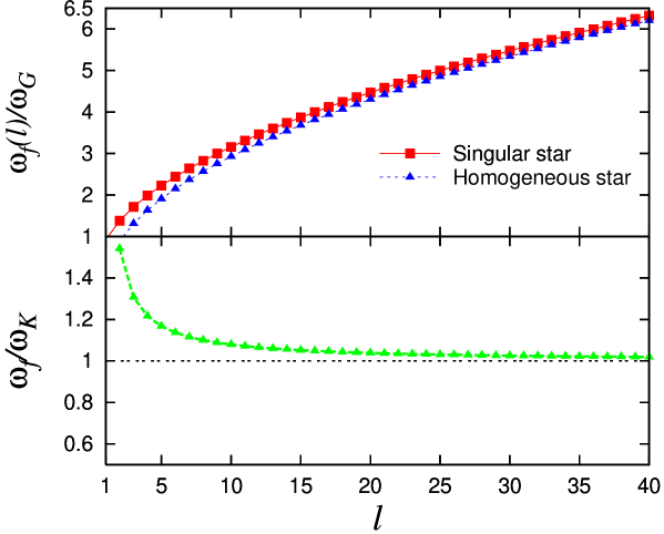
Figure 1: Frequency of fundamental modes $\omega_{f}$ as a function of multipole degree $l$ of global nodeless irrotational vibrations of singular and homogeneous star normalized to the natural unit of frequency $\omega_{G}$ (upper panel), and the ratio of spectral equations for the frequency of fundamental mode in singular model $\omega_{f}$ and in the Kelvin homogeneous model $\omega_{K}$.

The frequency spectrum of fundamental vibration mode in the singular star model reads

$$\omega_{f}^{2}(_{0}g_{\ell})=\omega^{2}_{G}\frac{2\ell(2\ell+1)-1}{2(2\ell+1)},\quad\quad\omega^{2}_{G}=\frac{4\pi}{3}\,G\,\rho_{s}=\frac{GM}{R^{3}},\quad\quad\ell\geq 1.$$ (67)

This last equation can be recast in the following equivalent form

$$\omega_{f}(_{0}g_{\ell})=\omega_{G}\left[\ell-\frac{1}{2(2\ell+1)}\right]^{1/2},$$ (68)

$$\ell>>1\quad\quad\omega_{f}(_{0}g_{\ell})\simeq\omega_{G}\sqrt{\ell}.$$ (69)

showing asymptotic behavior of the frequency at very high overtones.

The obtained frequency spectrum of $f$-mode in singular star model has many features in common with the well-known Kelvin spectral formula for kinematically identical fundamental vibration mode in homogeneous star model

$$\omega_{K}=\omega_{f}(_{0}g_{\ell})=\omega_{G}\left[\frac{2\ell(\ell-1)}{(2\ell+1)}\right]^{1/2},\quad\quad\omega_{G}=\sqrt{\frac{GM}{R^{3}}},\quad\quad\ell\geq 2$$ (70)

but the lowest overtone of Kelvin $f$-mode is of quadrupole degree, $\ell=2$. As is demonstrated in Fig.1, the most essential differences between the above spectral equations are manifested in low-overtone domain (upper panel) and that at large $\ell$ the frequency spectra of $f$-mode in singular and homogeneous star models shear identical asymptotic behavior (lower panel). In the next section this last spectral formula is briefly recovered by the above expounded method with allow for the effect of viscous damping of $f$-mode whose lifetime is computed with non-uniform profile of shear viscosity identical in appearance to that for the profile of hydrostatic pressure in this model.

4 Kelvin $f$-mode in the homogeneous liquid star

In the canonical homogeneous star model of uniform density, $\rho={\rm constant}$ the total mass has one and the same form as in above singular model, $M=(4\pi/3)\rho R^{3}$. The internal and external potentials of Newtonian gravitational field are the solutions of Poisson equation inside and Laplace equation outside the star

$$\nabla^{2}U_{i}=-4\pi\,G\rho:\,\,U_{i}(r<R)=2\pi G\rho R^{2}\left[1-\frac{1}{3}\left(\frac{r}{R}\right)^{2}\right]=\frac{3}{2}\frac{GM}{R}\left[1-\frac{1}{3}\left(\frac{r}{R}\right)^{2}\right],$$ (71)

$$W=\frac{1}{2}\int\rho\,U_{i}\,d{\cal V}=\frac{3}{5}\frac{GM^{2}}{R},\quad\nabla^{2}U_{e}=0:\,\,U_{e}(r>R)=\frac{4\pi}{3}G\rho\frac{R^{3}}{r}=\frac{GM}{r},$$ (72)

$${\rm\bf g}=-\nabla U:\quad{\rm\bf g}_{i}(r<R)=\frac{GM}{R^{3}}\,{\bf r},\quad\quad{\rm\bf g}_{e}(r>R)=\frac{G\,M}{r^{3}}\,{\bf r}.$$ (73)

In (72), $W$ is the internal gravitational energy $W$ of homogeneous star. The solution of equation of hydrostatic for pressure $p(r)$ is given by

$$\nabla p(r)=\rho\nabla U_{i}(r)\quad\to\quad p(r)=\frac{2\pi}{3}G\rho^{2}(R^{2}-r^{2})=P_{c}\left[1-\left(\frac{r}{R}\right)^{2}\right],$$ (74)

$$P_{c}=\frac{2\pi}{3}G\rho^{2}R^{2}=\frac{3}{8\pi}\frac{GM^{2}}{R^{4}},\quad R=\sqrt{\frac{3P_{c}}{{2\pi}{G\rho^{2}}}}.$$ (75)

The last expression shows again that the star radius is determined by the central pressure $P_{c}$ related to the density $\rho$ by equation of state.

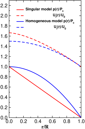
Figure 2: The fractional pressure and gravity potential profiles in singular inhomogeneous star model and in the canonical homogenous star model.

For comparison, in Fig.2 we plot the fractional pressure and gravity potential profiles computed in homogeneous model

$$\frac{p(r)}{P_{c}}=\left[1-\left(\frac{r}{R}\right)^{2}\right],\quad P_{c}=\frac{3}{8\pi}\frac{GM^{2}}{R^{4}},\quad\frac{U_{i}(r)}{U_{0}}=\frac{3}{2}\left[1-\frac{1}{3}\left(\frac{r}{R}\right)^{2}\right],\quad U_{0}=\frac{GM}{R}$$ (76)

and in singular inhomogeneous model

$$\frac{p(r)}{P_{c}}=\left(1-\frac{r}{R}\right),\quad P_{c}=\frac{5}{8\pi}\frac{GM^{2}}{R^{4}},\quad\frac{U_{i}(r)}{U_{0}}=\frac{5}{3}\left[1-\frac{2}{5}\left(\frac{r}{R}\right)^{3/2}\right],\quad U_{0}=\frac{GM}{R}.$$ (77)

The governing equations for non-compressional irrotational vibrations of the homogeneous liquid star are

$$\rho\delta{\dot{v}}_{i}=-\nabla_{i}\delta p+\rho\nabla_{i}\delta U+\nabla_{k}\delta\pi_{ik},$$ (78)

$$\delta{\dot{p}}=-(v_{k}\nabla_{k})\,p,\quad\nabla^{2}\delta U=0,$$ (79)

$$\delta\pi_{ik}=2\eta\delta v_{ik},\quad\delta v_{ik}=\frac{1}{2}(\nabla_{i}\delta v_{k}+\nabla_{k}\delta v_{i}),\quad\eta=\eta_{c}\left[1-\left(\frac{r}{R}\right)^{2}\right].$$ (80)

The equation of energy conservation is

$$\frac{\partial}{\partial t}\int\frac{\rho\delta v^{2}}{2}\,d{\cal V}=-\int[(\delta v_{k}\nabla_{k})\delta p-\rho(\delta v_{k}\nabla_{k})\delta U-\delta\pi_{ik}\delta v_{ik}]\,d{\cal V}.$$ (81)

On substituting here

$$\delta v_{i}({\bf r},t)=a_{i}({\bf r}){\dot{\alpha}}(t),\quad\delta U({\bf r},t)=\phi_{i}({\bf r}){\alpha}(t),\quad\delta p({\bf r},t)=-(a_{k}\nabla_{k})\,p(r){\alpha}(t)$$

we arrive at equation of damped oscillator, ${\cal M}{\ddot{\alpha}}+{\cal D}{\dot{\alpha}}+{\cal K}\alpha=0$, with integral parameters defining the frequency and lifetime of the form

$${\cal M} = \int_{\cal V}\rho\,a_{k}\,a_{k}\,d{\cal V},\quad{\cal D}=2\int\eta(r)a_{ik}\,a_{ik}\,d{\cal V},$$ (82)

$${\cal K} = -\int_{\cal V}[(a_{i}\nabla_{i})\,(a_{k}\nabla_{k})p(r)+\rho\,(a_{k}\,\nabla_{k})\phi({\bf r})]\,d{\cal V},$$ (84)

$$\omega^{2}=\frac{{\cal K}}{{\cal M}},\quad\tau=\frac{2{\cal M}}{{\cal D}}.$$

The only unknown quantity is the variations of the gravity potentials obeying the Laplace equations

$$\nabla^{2}\delta U_{i}=0,\quad\quad\nabla^{2}\delta U_{e}=0$$ (85)

having the general solutions of the form

$$\delta U_{i}(r<R)=C_{\ell}\,r^{\ell}P_{\ell}(\zeta)\alpha(t),\quad\quad\delta U_{e}(r<R)=D_{\ell}\,r^{-(\ell+1)}P_{\ell}(\zeta)\alpha(t).$$ (86)

The arbitrary constants $C_{\ell}$ and $D_{\ell}$ are eliminated from the standard boundary conditions

$$U_{i}(r(t))+\delta U_{i}(r(t))=U_{e}(r(t))+\delta U_{e}(r(t))\Big{|}_{R=R},$$ (87)

$$\frac{d}{dr}\left[U_{i}(r(t))+\delta U_{i}(r(t))\right]=\frac{d}{dr}\left[U_{e}(r(t))+\delta U_{e}(r(t))\right]\Big{|}_{r=R}$$ (88)

where $r(t)=r[1+\alpha(t)P_{\ell}(\cos\theta)]$. Retaining in these equations terms of first order in $\alpha(t)$ and putting $r=R$ we arrive at coupled algebraic equations for $C_{\ell}$ and $D_{\ell}$ whose solution leads to the following final expressions for the time-independent part of gravity potential (Bastrukov 1996a)

$$\phi_{i}=\frac{4\pi}{2l+1}\frac{G\rho}{R^{\ell-2}}\,r^{\ell}\,P_{\ell}(\zeta),\quad\phi_{e}=\frac{4\pi}{2\ell+1}G\rho\,R^{\ell+3}\,r^{-(\ell+1)}P_{\ell}(\zeta).$$ (89)

Computation of integral parameters of the inertia ${\cal M}$ viscous friction ${\cal D}$ yields

$${\cal M}=4\pi\,A^{2}_{\ell}\,\rho R^{2\ell+1}\frac{\ell}{2\ell+1}=\frac{4\pi\rho R^{5}}{\ell\left(2\ell+1\right)},$$ (91)

$${\cal D}=16\pi\,A_{\ell}^{2}\eta_{c}R^{2\ell-1}\frac{\ell(\ell-1)}{2\ell+1}=16\pi\eta_{c}R^{3}\frac{(\ell-1)}{2\ell+1}.$$

Following the suggestion of Cowling (1941), one can consider separately oscillations restored by force associated with gradient in fluctuations of pressure and force owing its origin to fluctuations in the potential of gravity. In accord with this, the integral parameter of stiffness is written represents as a sum

$${\cal K}={\cal K}_{p}+{\cal K}_{g},$$ (92)

$${\cal K}_{p}=-\int_{\cal V}(a_{k}\nabla_{k})\,(a_{i}\nabla_{i})p(r)\,d{\cal V},\quad{\cal K}_{g}=-\int_{\cal V}\rho(a_{i}\nabla_{i})\phi({\bf r})\,d{\cal V}$$ (93)

and, consequently, the frequency frequency of vibrations is also represented as a sum

$$\omega^{2}=\omega_{p}^{2}+\omega_{g}^{2},\quad\omega_{p}^{2}=\frac{{\cal K}_{p}}{\cal M},\quad\omega_{g}^{2}=\frac{{\cal K}_{g}}{\cal M}$$ (94)

where $\omega_{p}$ designate the frequency of $p$-mode and $\omega_{g}$ is the frequency of $g$-mode. For ${\cal K}_{p}$ and ${\cal K}_{g}$ we get

$${\cal K}_{p}=\frac{16\pi^{2}}{3}\frac{G\rho^{2}R^{5}}{2\ell+1},\quad{\cal K}_{g}=-\frac{16\pi^{2}G\rho^{2}R^{5}}{(2\ell+1)^{2}}.$$ (95)

For the frequencies of $p$-mode and $g$ mode we obtain

$$\omega_{p}^{2}=\frac{{\cal K}_{p}}{\cal M}=\omega_{G}^{2}\,\ell,\quad\quad\omega_{g}^{2}=\frac{{\cal K}_{g}}{\cal M}=-\omega_{G}^{2}\frac{3\ell}{2\ell+1}.$$ (96)

One sees that $\omega_{p}^{2}$ is positive whereas $\omega_{g}^{2}$ is negative. It follows that frequency of fundamental mode $\omega_{f}(_{0}g_{\ell})=[\omega_{p}^{2}+\omega_{g}^{2}]^{1/2}$ is given by Kelvin spectral formula (70) and for the lifetime of $\ell$-pole overtone, $\tau_{f}(\ell)$, computed with the non-uniform radial profile of shear viscosity $\eta=\eta(r)$ given by equation (80), we obtain

$$\tau_{f}(\ell)=\frac{\tau_{\nu}}{2(l-1)},\quad\quad\tau_{\nu}=\frac{R^{2}}{\nu},\quad\nu=\frac{\eta_{c}}{\rho}.$$ (97)

Figure 3: The fractional lifetime of $\ell$-pole overtones of fundamental vibrational mode in homogeneous and inhomogeneous liquid star models with non-uniform profiles of shear viscosity in juxtaposition with Lamb spectral equation for damping time of nodeless irrotational oscillations of a spherical mass of viscous liquid of uniform density and constant coefficient of shear viscosity.

It is worthwhile to compare the computed lifetime spectra with the Lamb (1945) spectral equation

$$\tau_{\rm Lamb}(\ell)=\frac{\tau_{\nu}}{(2\ell+1)(l-1)}$$ (98)

that has been obtained in a similar fashion but assuming that coefficient of shear viscosity has constant value in the entire spherical volume of homogeneous viscous liquid (see also Bastrukov et al 2007). It has been pointed by Jeffreys (1976), however, in the context of geoseismology that the approximation of uniform viscosity does not allows for the effect of self-gravity on mechanical property of matter of astrophysical objects. With this in mind, we have supposed that it would be not inconsistent to take radial profile of shear viscosity similar to that for hydrostatic pressure in the star. Also noteworthy is that Newtonian law of shear viscosity is equally appropriate for viscous liquid and viscoelastic solid (e.g. Landau et al 1986). The obtained here spectral equations for the time of viscose damping of nodeless spheroidal vibrations may be of some interest, therefore, for the general seismology of Earth-like planet (Aki & Richards 2002). In Fig.3, the obtained spectral equations for the lifetime, normalized to $\tau_{\nu}$, as a function of overtone number $\ell$ are plotted for both singular (61) and homogeneous (97) models in juxtaposition with the Lamb spectral formula (98).

5 Summary

The most striking differences between vibrational behavior of homogenous and inhomogeneous liquid star models in the fundamental mode of global nodeless irrotational pulsations under the combined action of the buoyancy and gravity forces is that in the inhomogeneous model the oscillations are of substantially compressional character, that is, accompanied by fluctuations in density and the lowest overtone of $f$-mode is of dipole degree, as has first been observed in (Podgainy et al 1996). In the homogeneous star model they are characterized as non-compressional and the lowest overtone is of quadrupole degree.

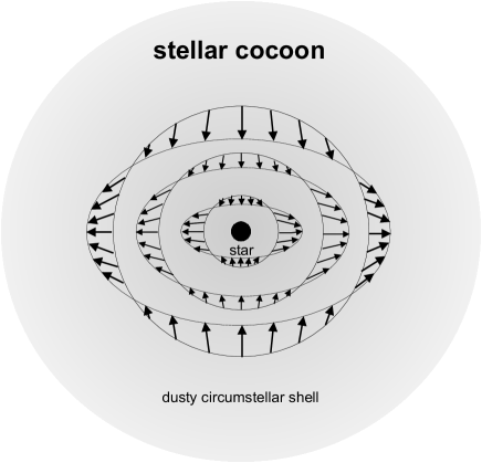
Figure 4: Artist view of a spherical star-forming object, the stellar cocoon, whose largescale vibrations in $f$-mode can be analyzed on the basis considered highly inhomogeneous model.

The natural unit of frequency of $f$-mode, $\omega_{G}=\sqrt{GM/R^{3}}$, has one and the same form as that for gravity or $g$-modes. These letter modes are of particular importance for the asteroseismology of transitory pre-white dwarfs objects and young white dwarfs (e.g. Hansen & Kawaler 1994) whose variability of electromagnetic emission is attributed to non-radial gravity-driven seismic vibrations (Koester & Chanmugam 1990, Fontaine & Brassard 2008, Winget & Kepler 2008). To this end, it is worth emphasizing, the existing modal classification of the $g$-mode spectra presumes that white-dwarf-forming object oscillates in the standing-wave regime in which the frequency is determined by nodal structure of fluctuating variables (e.g. Unno et al 1989, Winget & Kepler 2008). According to standard nomenclature, the $g$-modes of standing-wave regime of non-radial pulsations are specified as ${}_{n}g_{\ell}$, where $n\geq 1$ is the node number and $\ell$ is the multipole degree of overtone. In the meantime, the regime of nodeless oscillations, designated as ${}_{0}g_{\ell}$, remains less studied. Also, the considered model can be invoked in assessing variability of emission from star-forming clouds like stellar cocoon, pictured in Fig.4, as caused by its vibrations in fundamental mode. Motivated by these arguments we have investigated an analytic model of a highly inhomogeneous star undergoing global nodeless irrotational vibrations. In work (Bastrukov 1996b) these kind of nodeless oscillations have been studied in the model of homogeneous liquid layer. In recent papers (Bastrukov et al 2007b, 2008), the nodeless vibrations of a solid star driven by restoring force of elastic deformations and locked in the peripheral finite-depth mantle, has been been studied in the context of seismic vibrations of the neutron star crust in the approximation of uniform density of crustal matter. Understandably that in real white dwarfs and neutron stars the bulk density is non-homogeneous function of position. However, this realistic case of nodeless irrotational vibrations entrapped in the peripheral finite-depth seismogenic layer with non-uniform density profile demands more elaborate mathematical treatment which will be the subject of our forthcoming paper.

References

(1) Aki K & Richards P G 2002 Quantitative Seismology (Mill-Valley, CA: University Science Books)
(2) Bastrukov S I 1996a Phys. Rev. E 53 1917
(3) Bastrukov S I 1996b Int. J. Mod. Phys. D 5 45
(4) Bastrukov S I, Chang H-K, Mişicu Ş, Molodtsova I V & Podgainy D V
2007a Int. J. Mod. Phys. A 22 3261
(5) Bastrukov S I, Chang H-K, Takata J, Chen G-T & Molodtsova I V 2007b Mon. Not.
R. Astron. Soc.382 849
(6) Bastrukov S I, Chang, H-K, Chen, G-T & Molodtsova I V 2008 Mod. Phys. Lett. A 23 477
(7) Chandrasekhar S 1961 Hydrodynamic and Hydromagnetic Stability
(Oxford: Clarendon)
(8) Clayton D D 1986 Am. J. Phys.54 354
(9) Cowling T G 1941 Mon. Not. R. Astron. Soc.101 367
(10) Cox J P 1980 Theory of Stellar Pulsation (Princeton: Princeton University Press)
(11) Fontaine G & Brassard P 2008 Publ. Astron. Soc. Pacific120 1043
(12) Jeffreys H 1976 The Earth 6th ed (Cambridge: Cambridge University Press).
(13) Hansen C J & Kawaler S D 1994 Stellar Interiors (New York: Springer-Verlag)
(14) Huang K 1987 Statistical mechanics 2d ed (New York: Wiley)
(15) Koester D & Chanmigam G 1990 Rep. Prog. Phys.53 837
(16) Lamb H 1945 Hydrodynamics (New York: Dover)
(17) Landau L D, Lifshits E M, Kosevich A M & Pitaevskii L P 1986 Theory of
Elasticity 3d ed (Oxford: Pergamon)
(18) Phillips A C 1994 The Physics of Stars (New York: Wiley)
(19) Podgainy D V, Bastrukov S I, Molodtsova I V & Papoyan V V 1996
Astrophys.39 278
(20) Thompson W (Kelvin) 1863 Phil. Trans. (papers iii, 384)
(21) Unno W, Osaki Y, Ando H, Saio H & Shibahashi H 1989 Nonradial Oscillations
of Stars 2d ed (Tokyo: Tokyo University Press)
(22) Winget D E & Kepler S O 2008 Annu. Rev. Astron. Astrophys.46 157