Zero Dispersion and Zero Dissipation Implicit Runge-Kutta Methods for the Numerical Solution of Oscillating IVPs

Abstract

In this paper we present two new methods based on an implicit Runge-Kutta method Gauss which is of algebraic order fourth and has two stages: the first one has zero dispersion and the second one has zero dispersion and zero dissipation. The efficiency of these methods is measured while integrating the radial Schrödinger equation and other well known initial value problems.

1 Introduction

We consider the radial Schrödinger equation:

$$y^{\prime\prime}(x)=\left[\frac{l(l+1)}{x^{2}}+V(x)-E\right]y(x)$$ (1)

where $\frac{l(l+1)}{x^{2}}$ is the centrifugal potential, $V(x)$ is the potential, $E$ is the energy and $W(x)=\frac{l(l+1)}{x^{2}}+V(x)$ is the effective potential. It is valid that

$$\lim_{\upsilon\rightarrow\infty}{V(x)}=0$$

and therefore

$$\lim_{\upsilon\rightarrow\infty}{W(x)}=0.$$

We will study the case of $E>0$.

If we divide $[0,\infty]$ into small subintervals $[a_{i},b_{i}]$ so that $W(x)$ is considered constant with value $\bar{W_{i}}$, then the problem (1) is reduced to the approximation

$y^{\prime\prime}_{i}=\left(\bar{W}-E\right)y_{i}$, whose solution is

$$y_{i}(x)=A_{i}\,\ exp\left(\sqrt{\bar{W}-E}x\right)+B_{i}\,\ exp\left(-\sqrt{\bar{W}-E}x\right),\quad A_{i},B_{i}\in\Re.$$ (2)

This form of Schrödinger equation shows why phase fittin is so important when new methods are constructed. In the next section we will present the most important parts of the theory used.

The structure of the paper is as follows. Firstly in section 2, the basic theory of implicit Runge-Kutta methods is presented. In section 3, the construction of the methods is introduced. In section 4 and 5, the calculation of the algebraic order and the symplecticity respectively of the new methods is given. Then in section 6, the numerical results of the new methods are presented compared to classical RK methods from the literature while integrating well known initial value problems and the radial Schrödinger equation. Finally in section 7 our conclusions are presented.

2 Basic Theory

2.1 Implicit Method.

The general form of an s-stage implicit Runge-Kutta method used for the computation of the approximate value of $y_{n+1}(x)$ in Problem (1), when $y_{n}(x)$ is known, is given from the following procedure:

$$\begin{array}[]{l}w_{i}=f(t_{n}+c_{i}h,y_{n}+h\sum\limits_{j=1}^{s}a_{ij}w_{j})\\ y_{n+1}=y_{n}+h\sum\limits_{i=1}^{s}b_{i}w_{i}\end{array}$$ (3)

when at least one $a_{ij}\neq 0$ exists with $i\leq j$.

An implicit Runge-Kutta method can also be presented using the Butcher table below:

$$\begin{array}[]{l|llllll}c_{1}&a_{11}&a_{12}&...&a_{1s-1}&a_{1s}\\ c_{2}&a_{21}&a_{22}&...&a_{2s-1}&a_{2s}\\ c_{3}&a_{31}&a_{32}&...&a_{3s-1}&a_{3s}\\ \vdots&\vdots&\vdots&\ddots&\vdots&\vdots\\ c_{s}&a_{s1}&a_{s2}&...&a_{s,s-1}&a_{ss}\\ \hline\cr&b_{1}&b_{2}&...&b_{s-1}&b_{s}\end{array}$$ (4)

2.2 Phase-Lag Analysis

Let A and B, $s\times s$ matrices, be defined by $A=(a_{ij}),\quad(1\leq i,j\leq s$) and $B=(a_{ij}-b_{j}),\quad(1\leq i,j\leq s)$ respectively. When the method (3) is applied to the linear equation

$$y^{\prime}=qy,\quad q\in C$$ (5)

the numerical solution is given by

$$y_{n+1}=P(z)y_{n},\quad P(z)=\frac{det(I-zB)}{det(I-zA)}$$ (6)

and can be written in the form

$$P(z)=K(\upsilon)+iL(\upsilon),\quad z=hq$$ (7)

where $K(\upsilon)$ and $L(\upsilon)$ are functions of $\upsilon$ and $i=\sqrt{-1}$.

Definition 1

[6] In the implicit s-stage Runge-Kutta method, presented in (4), the quantities

$$\phi(\upsilon)=\upsilon-arg(P(i\upsilon)),\quad\alpha(\upsilon)=1-|P(i\upsilon)|,\quad\upsilon\in\ \Re$$ (8)

are respectively called the phase-lag or dispersion error and the dissipative error. If $\phi(\upsilon)=O(\upsilon^{q+1})$ and $\alpha(\upsilon)=O(\upsilon^{r+1})$ then the method is said to be of dispersive order $q$ and dissipative order $r$.

2.3 Stability

Definition 2

[15] The stability function for an implicit Runge-Kutta method is the rational function

$$R(z)=\frac{det(I-zA+zeb^{T})}{det(I-zA)},$$ (9)

where the vector $e=(1,...,1)^{T}$, and that a method is A-stable if $|R(z)|\leq 1$,  whenever $Re(z)\leq 0$, where $Re(z)$ is the real part of $z$.

3 Construction of the new Runge-Kutta methods

We consider the implicit Runge-Kutta method of Gauss, which is of algebraic order fourth and has two stages. The coefficients are shown in Table 10.

$$\begin{array}[]{l|lll}\frac{1}{2}-\frac{\sqrt{3}}{6}&\frac{1}{4}&\frac{1}{4}-\frac{\sqrt{3}}{6}\\ \frac{1}{2}+\frac{\sqrt{3}}{6}&\frac{1}{4}+\frac{\sqrt{3}}{6}&\frac{1}{4}\\ \hline\cr&\frac{1}{2}&\frac{1}{2}\end{array}$$ (10)

Below we present the construction of the methods.

3.1 Construction of the new method with zero phase lag

We consider all the values of Table 10 except $b_{2}$. By evaluating the phase-lag of this method, defined in Definition 1, and by solving $\phi(v)=0$ towards $b_{2}$, the result is:

$$\begin{array}[]{l}\displaystyle b_{2}=\frac{1}{2}\,{\frac{-6\,{\,\upsilon}^{3}+6\,{\,\upsilon}^{3}\,\sqrt{3}+72\,\,\upsilon-\,\mathrm{tan}\left(\,\upsilon\right){\,\upsilon}^{4}+24\,\,\mathrm{tan}\left(\,\upsilon\right){\,\upsilon}^{2}}{\,\mathrm{tan}\left(\,\upsilon\right)\,\sqrt{3}{\,\upsilon}^{4}+6\,{\,\upsilon}^{3}+6\,{\,\upsilon}^{3}\,\sqrt{3}}}\\ \displaystyle\qquad\frac{+\tan\left(\upsilon\right){\upsilon}^{4}\sqrt{3}-12\,\mathrm{tan}\left(\upsilon\right){\upsilon}^{2}\sqrt{3}-144\,\mathrm{tan}\left(\upsilon\right)}{-36\,\upsilon^{2}\,\mathrm{tan}\left(\upsilon\right)-12\,\upsilon^{2}\,\mathrm{tan}\left(\upsilon\right)\sqrt{3}-72\,\upsilon}\end{array}$$ (11)

The Taylor series expansion of $b_{2}$ is shown below:

$$\begin{array}[]{l}\displaystyle b_{2_{taylor}}=\ \frac{1}{2}\ +\ {\frac{1}{720}}\,{\upsilon}^{4}\ +\ \left({\ \frac{1}{6720}}\ -\ {\frac{1}{8640}}\,\sqrt{3}\ \right){\upsilon}^{6}\ \ +\ldots\end{array}$$

In the last equation we observe that

$$\lim_{\upsilon\rightarrow 0}{b_{2_{taylor}}}=\frac{1}{2}$$

namely when the step-length tends to zero the coefficient of the method Gauss appears.

3.2 Construction of the new method with zero phase lag and zero dissipation

We consider all the values of Table 10 except two: $b_{2}$ and $a_{22}$. An extra equation (apart from the equation of the phase lag) must hold, in order to achieve zero phase-lag and zero dissipation. The two equations are $\phi(v)=0$ and $\alpha(v)=0$.

After satisfying the above two equations, by solving towards $b_{2}$ and $a_{22}$, the result is:

$$\begin{array}[]{l}\displaystyle{b_{2}}=\frac{1}{6}\cdot\frac{A}{B}\end{array}$$ (13)

where

$$\displaystyle A = -24\,\sin\left(\upsilon\right)\upsilon\,\sqrt{3}+2\,\sin\left(\upsilon\right){\upsilon}^{3}\sqrt{3}+12\,{\upsilon}^{2}\cos\left(\upsilon\right)$$

$$-36\,\sin\left(\upsilon\right)\upsilon-3\,\sin\left(\upsilon\right){\upsilon}^{3}-144\,\cos\left(\upsilon\right)$$

$$+12\,\sqrt{-{\frac{-4\,{\upsilon}^{4}+2\,{\upsilon}^{4}\sqrt{3}+24\,{\upsilon}^{2}-24\,{\upsilon}^{2}\sqrt{3}-144}{\left(\cos\left(\upsilon\right)\right)^{2}}}}\cos\left(\upsilon\right)$$

$$\displaystyle B={\upsilon}\left(4\,\upsilon\,\sqrt{3}\cos\left(\upsilon\right)+\sin\left(\upsilon\right){\upsilon}^{2}-12\,\sin\left(\upsilon\right)\right)$$

and

$$\begin{array}[]{l}\displaystyle{a_{22}}=-\frac{1}{12}\cdot\frac{C}{D}\end{array}$$ (14)

with

$$\displaystyle D = -144\,{\upsilon}^{4}\left(\cos\left(\upsilon\right)\right)^{2}-6\,{\upsilon}^{6}\left(\cos\left(\upsilon\right)\right)^{2}+576\,{\upsilon}{2}\,\sqrt{3}+864\,{\upsilon}^{2}$$

$$-144\,\sin\left(\upsilon\right){\upsilon}^{3}\sqrt{3}\cos\left(\upsilon\right)-2\,{\upsilon}^{6}\sqrt{3}-6\,{\upsilon}^{5}+120\,{\upsilon}^{4}\left(\cos\left(\upsilon\right)\right)^{3}\sqrt{3}$$

$$-36\,{\upsilon}^{5}\cos\left(\upsilon\right)\sin\left(\upsilon\right)-1728\,{\upsilon}^{2}\,\sqrt{3}\left(\cos\left(\upsilon\right)\right)^{2}$$

$$-24\,\sin\left(\upsilon\right){\upsilon}^{5}\sqrt{3}\cos\left(\upsilon\right)-1152\,{\upsilon}^{3}\cos\left(\upsilon\right)\sin\left(\upsilon\right)$$

$$+3456\,\cos\left(\upsilon\right)\sin\left(\upsilon\right)\,{\upsilon}+96\,{\upsilon}^{2}\,\sqrt{3}\left(\cos\left(\upsilon\right)\right)^{2}-{\upsilon}^{7}\sin\left(\upsilon\right)\sqrt{3}\cos\left(\upsilon\right)$$

$$+24T_{0}\,\sin\left(\upsilon\right){\upsilon}^{3}\cos\left(\upsilon\right)+12\,{\upsilon}^{4}\left(\cos\left(\upsilon\right)\right)^{2}$$

$$+14\,{\upsilon}^{6}\sqrt{3}\left(\cos\left(\upsilon\right)\right)^{2}+3\,{\upsilon}^{7}\sin\left(\upsilon\right)\cos\left(\upsilon\right)$$

$$+{\upsilon}^{6}\sin\left(\upsilon\right)\sqrt{3}\cos\left(\upsilon\right)-12\,\sin\left(\upsilon\right){\upsilon}^{4}\sqrt{3}\cos\left(\upsilon\right)$$

$$-288\,\sin\left(\upsilon\right)\cos\left(\upsilon\right)-24\,{\upsilon}^{3}\sqrt{3}-864\,\upsilon\,\left(\cos\left(\upsilon\right)\right)^{2}$$

where

$$\displaystyle T_{0}=\sqrt{-{\frac{2\,{\upsilon}^{4}\sqrt{3}-4\,{\upsilon}^{4}+24\,{\upsilon}^{2}-24\,{\upsilon}^{2}\sqrt{3}-144}{\left(\cos\left(\upsilon\right)\right)^{2}}}}$$

The Taylor series expansion of $b_{2}$ and $a_{22}$ are shown below:

$$\displaystyle b_{2_{taylor}}={\frac{1}{2}}+{\frac{1}{720}}\,{\upsilon}^{4}+{\frac{1}{10080}}\,{\frac{5\,\sqrt{3}-8}{-3+\sqrt{3}}}\,{\upsilon}^{6}+\ldots$$

$$\displaystyle a_{22_{taylor}}={\frac{1}{4}}+{\frac{1}{2160}}\,{\frac{5\,\sqrt{3}-9}{-2+\sqrt{3}}}\,{\upsilon}^{4}-{\frac{1}{181440}}\,{\frac{220\,\sqrt{3}-381}{\left(-2+\sqrt{3}\right)^{2}}}\,{\upsilon}^{6}+\ldots$$

In the last equations we observe that the limits when $\upsilon\rightarrow 0$ are equal to the corresponding coefficients of the Gauss method.

4 Algebraic order of the new methods

The following 8 equations must be satisfied so that the new method maintains the fourth algebraic order of the corresponding classical method presented in Table 10. The number of stages is symbolized by $s$, where $s=2$.

$$\begin{array}[]{cc}\textbf{1st Alg. Order (1 equation)}\\ {\sum\limits_{i=1}^{s}{b_{i}}}=1\end{array}$$ (17)

$$\begin{array}[]{cc}\textbf{2st Alg. Order (2 equations)}\\ {\sum\limits_{i=1}^{s}{b_{i}}}c_{i}=\frac{1}{2}\end{array}$$ (20)

$$\begin{array}[]{cc}\textbf{3st Alg. Order (4 equations)}\\ {\sum\limits_{i=1}^{s}{b_{i}}}c_{i}^{2}=\frac{1}{3}\\ {\sum\limits_{i,j=1}^{s}{b_{i}}}a_{ij}c_{j}=\frac{1}{6}\end{array}$$ (24)

$$\begin{array}[]{cc}\textbf{4st Alg.Order (8 equations)}\\ {\sum\limits_{i=1}^{s}{b_{i}}}c_{i}^{3}=\frac{1}{4}\\ {\sum\limits_{i,j=1}^{s}{b_{i}}}c_{i}a_{ij}c_{j}=\frac{1}{8}\\ {\sum\limits_{i,j=1}^{s}{b_{i}}}a_{ij}c_{j}^{2}=\frac{1}{12}\\ {\sum\limits_{i,j,k=1}^{s}{b_{i}}}a_{ij}a_{jk}c_{k}=\frac{1}{24}\end{array}$$ (30)

4.1 Remainders for the first method (algebraic conditions)

We present the remainders of the eight equations, that is the difference of the right part minus the left part, for the first method:

$$\begin{array}[]{l}rem_{1}={\frac{1}{720}}\,\,{\upsilon}^{4}+\left({\frac{1}{6720}}-{\frac{1}{8640}}\,\sqrt{3}\right){\upsilon}^{6}+\ldots\\ rem_{2}=\left({\frac{1}{1440}}\,+{\frac{\sqrt{3}}{4320}}\,\,\right){\upsilon}^{4}+\,\left({\frac{1}{60480}}\,-{\frac{\sqrt{3}}{30240}}\,\,\right){\upsilon}^{6}+\ldots\\ rem_{3}=\left({\frac{1}{2160}}\,+{\frac{\sqrt{3}}{4320}}\,\,\right){\upsilon}^{4}-\,\left({\frac{1}{120960}}\,-{\frac{\sqrt{3}}{72576}}\,\,\right){\upsilon}^{6}+\ldots\\ rem_{4}=\left({\frac{1}{4320}}\,+{\frac{\sqrt{3}}{8640}}\,\,\right){\upsilon}^{4}-\,\left({\frac{1}{241920}}\,-{\frac{\sqrt{3}}{145152}}\,\,\right){\upsilon}^{6}+\ldots\\ rem_{5}=\left({\frac{1}{2880}}\,+{\frac{\sqrt{3}}{5184}}\,\,\right){\upsilon}^{4}-\,\left({\frac{1}{90720}}\,-{\frac{\sqrt{3}}{120960}}\,\,\right){\upsilon}^{6}+\ldots\\ rem_{6}=\,\left({\frac{1}{5760}}\,+{\frac{\sqrt{3}}{10368}}\,\,\right){\upsilon}^{4}-\,\left({\frac{1}{181440}}\,-{\frac{\sqrt{3}}{241920}}\right)\,{\upsilon}^{6}+\ldots\\ rem_{7}=\,\left({\frac{1}{8640}}\,+{\frac{\sqrt{3}}{12960}}\,\,\right){\upsilon}^{4}-\,\left({\frac{1}{145152}}\,-{\frac{\sqrt{3}}{725760}}\right)\,\,{\upsilon}^{6}+\ldots\\ rem_{8}=\left({\frac{1}{17280}}\,+{\frac{\sqrt{3}}{25920}}\,\,\right){\upsilon}^{4}-\,\left({\frac{1}{290304}}\,-{\frac{\sqrt{3}}{1451520}}\,\,\right){\upsilon}^{6}+\ldots\\ \end{array}$$ (39)

We see that the eight equations are held, when $h\rightarrow 0\Rightarrow v\rightarrow 0$. This means that the new method maintains the algebraic order of the corresponding classical method.

4.2 Remainders for the second method (algebraic conditions)

Now we present the remainders of the equations for the second method:

$$\begin{array}[]{l}rem_{1}={\frac{1}{720}}\,{\upsilon}^{4}+{\frac{1}{10080}}\,{\frac{-8+5\,\sqrt{3}}{\sqrt{3}-3}}\,{\upsilon}^{6}+\ldots\\ rem_{2}=\left({\frac{1}{1440}}+{\frac{1}{4320}}\,\sqrt{3}\right){\upsilon}^{4}+{\frac{1}{60480}}\,{\frac{\left(-8+5\,\sqrt{3}\right)\left(3+\sqrt{3}\right)}{\sqrt{3}-3}}\,\,{\upsilon}^{6}+\ldots\\ rem_{3}={\frac{1}{25920}}\,\left(3+\sqrt{3}\right)^{2}{\upsilon}^{4}+{\frac{1}{362880}}\,{\frac{\left(-8+5\,\sqrt{3}\right)\left(3+\sqrt{3}\right)^{2}}{\sqrt{3}-3}}\,\,{\upsilon}^{6}+\ldots\\ rem_{4}=-{\frac{1}{8640}}\,{\frac{11\,\sqrt{3}-21}{\left(\sqrt{3}-3\right)\left(-2+\sqrt{3}\right)}}\,\,{\upsilon}^{4}+{\frac{1}{181440}}\,{\frac{137\,\sqrt{3}-237}{\left(\sqrt{3}-3\right)\left(-2+\sqrt{3}\right)^{2}}}\,\,{\upsilon}^{6}+\ldots\\ rem_{5}={\frac{1}{155520}}\,\left(3+\sqrt{3}\right)^{3}{\upsilon}^{4}+{\frac{1}{2177280}}\,{\frac{\left(-8+5\,\sqrt{3}\right)\left(3+\sqrt{3}\right)^{3}}{\sqrt{3}-3}}\,\,{\upsilon}^{6}+\ldots\\ rem_{6}=-{\frac{1}{51840}}\,{\frac{\left(3+\sqrt{3}\right)\left(11\,\sqrt{3}-21\right)}{\left(\sqrt{3}-3\right)\left(-2+\sqrt{3}\right)}}\,\,{\upsilon}^{4}+{\frac{1}{1088640}}\,{\frac{\left(3+\sqrt{3}\right)\left(137\,\sqrt{3}-237\right)}{\left(\sqrt{3}-3\right)\left(-2+\sqrt{3}\right)^{2}}}\,\,{\upsilon}^{6}+\ldots\\ rem_{7}=-{\frac{1}{8640}}\,\left(-2+\sqrt{3}\right)^{-1}{\upsilon}^{4}+{\frac{1}{725760}}\,{\frac{-53+31\,\sqrt{3}}{\left(\sqrt{3}-3\right)\left(-2+\sqrt{3}\right)^{2}}}\,\,{\upsilon}^{6}+\ldots\\ rem_{8}=-{\frac{1}{17280}}\,{\frac{3385\,\sqrt{3}-5863}{\left(\sqrt{3}-3\right)\left(-2+\sqrt{3}\right)^{5}}}\,\,{\upsilon}^{4}+{\frac{1}{290304}}\,{\frac{28121\,\sqrt{3}-48707}{\left(\sqrt{3}-3\right)\left(-2+\sqrt{3}\right)^{6}}}\,\,{\upsilon}^{6}+\ldots\\ \end{array}$$ (48)

We see that for $\upsilon=0$ the eight equations are held for this method too. Thus the new method has also fourth algebraic order.

5 Symplecticity of the new methods

Theorem The Runge-Kutta method (3)-(4) is symplectic when the following equalities are satisfied

$$b_{i}a_{ij}+b_{j}a_{ji}=b_{i}b_{j},\qquad 1\leq i,j\leq s.$$ (49)

As a classical example we mention the Gauss methods as symplectic Runge-Kutta methods. It should be noted that symplectic Runge-Kutta methods are always implicit.

Thus according to the above theorem, the three equations must be satisfied so that the symplecticity of the new methods will be maintained.

$$b_{1}a_{11}+b_{1}a_{11}=b_{1}b_{1}$$ (50)

$$b_{2}a_{22}+b_{2}a_{22}=b_{2}b_{2}$$ (51)

$$b_{1}a_{12}+b_{2}a_{21}=b_{1}b_{2}$$ (52)

5.1 Remainders for the first method (simplecticity conditions)

We present the remainder of the three equations, that is the difference of the right part minus the left part, for the first method:

$$\begin{array}[]{l}rem_{1}=0\\ rem_{2}=-{\frac{1}{1440}}\,{\upsilon}^{4}+\left(-{\frac{1}{13440}}+{\frac{1}{17280}}\,\sqrt{3}\right){\upsilon}^{6}+\ldots\\ rem_{3}=\left(-{\frac{1}{2880}}+{\frac{1}{4320}}\,\sqrt{3}\right){\upsilon}^{4}+\left(-{\frac{23}{241920}}+{\frac{13}{241920}}\,\sqrt{3}\right){\upsilon}^{6}+\ldots\\ \end{array}$$ (56)

We see that for the three equations are held, when $h\rightarrow 0\Rightarrow v\rightarrow 0$. That means that the new method maintains the symplecticity of the corresponding classical method.

5.2 Remainders for the second method (simplecticity conditions)

Now we present the remainders of the equations for the second method:

$$\begin{array}[]{l}rem_{1}=0\\ rem_{2}={\frac{1}{720}}\,{\frac{-45+26\,\sqrt{3}}{\left(-2+\sqrt{3}\right)\left(-3+\sqrt{3}\right)^{2}}}\,{\upsilon}^{4}+{\frac{1}{10080}}\,{\frac{545\,\sqrt{3}-944}{\left(-2+\sqrt{3}\right)^{2}\left(-3+\sqrt{3}\right)^{3}}}\,{\upsilon}^{6}+\ldots\\ rem_{3}=-{\frac{1}{2880}}\,{\frac{-5+3\,\sqrt{3}}{-3+\sqrt{3}}}\,{\upsilon}^{4}-{\frac{1}{120960}}\,{\frac{-54+31\,\sqrt{3}}{-3+\sqrt{3}}}\,{\upsilon}^{6}+\ldots\\ \end{array}$$ (60)

We see that for $\upsilon=0$ the three equations are held for this method too. Thus the new method is also symplectic.

6 Numerical Results

6.1 The methods

In order to measure the efficiency of the methods constructed in this paper we compare them to some already known methods, presenting the results of the best six.

I.   Method G2-PL-D constructed in this paper, where G2-PL-D means the method Gauss two-stages, fourth-order with zero phase-lag and zero dissipation.

II.  Method G2-PL constructed in this paper, where G2-PL means the method Gauss two-stage, fourth-order with zero phase-lag.

III.   Method G2: The classical two-stages and fourth-order Gauss method (see [16]).

IV. Method SDIRK(3,6,3): The Singly Diagonally-Implicit Runge-Kutta method of J. M. Franco, I. Gomez, L. Randez, is third-stage, third algebraic order,sixth dispersive order and third dissipative order (see [25]).

V.     Method Radau I: The classical third order Radau method (see [15]).

VI. Method Lobatto IIIC: The classical fourth order Lobatto method (see [15]).

6.2 The Problems

6.2.1 Inverse Resonance Problem

The efficiency of the two new constructed methods will be measured through the integration of problem (1) with $l=0$ at the interval $[0,15]$ using the well known Woods-Saxon potential

$$\begin{array}[]{l}\displaystyle V(x)=\frac{u_{0}}{1+q}+\frac{u_{1}q}{(1+q)^{2}},\quad q=exp\left(\frac{x-x_{0}}{a}\right),\end{array}$$ (62)

where  $u_{0}=-50,\quad a=0.6,\quad x_{0}=7\quad$ and $\quad\displaystyle u_{1}=-\frac{u_{0}}{a}$

and with boundary condition $y(0)=0$.

The potential $V(x)$ decays more quickly than $\displaystyle\frac{l(l+1)}{x^{2}}$ , so for large $x$ (asymptotic region) the Schrödinger equation (1) becomes

$$y^{\prime\prime}(x)=\left[\frac{l(l+1)}{x^{2}}+V(x)-E\right]y(x)$$ (63)

The last equation has two linearly independent solutions $\displaystyle k$$x$$j_{l}(kx)$ and $\displaystyle kxn_{l}(kx)$, where $j_{l}$ and $n_{l}$ are the spherical Bessel and Neumann functions. When $\displaystyle x\rightarrow\infty$ the solution takes the asymptotic form

$$\displaystyle y(x) \approx Akxj_{l}(kx)-Bkxn_{l}(kx)$$ (64)

$$\approx \displaystyle D\left[sin(kx-\pi l/2)+tan(\delta_{l})cos(kx-\pi l/2)\right]$$ (65)

where $\delta_{l}$ is called scattering phase shift and it is given by the following expression:

$$tan(\delta_{l})=\frac{y(x_{i})S(x_{i+1})-y(x_{i+1})S(x_{i})}{y(x_{i+1})C(x_{i})-y(x_{i})C(x_{i+1})}$$ (66)

where $\displaystyle S(x)=kxj_{l}(kx)$, $\displaystyle C(x)=kxn_{l}(kx)$ and $x_{i}<x_{i+1}$ and both belong to the asymptotic region. Given the energy we approximate the phase shift, the accurate value of which is $\pi/2$ for the above problem. We will use two values for the energy: $989.701916$ and $341.495874$. As for the frequency $w$ we will use the suggestion of Ixaru and Rizea in [2] and [4].:

$$w=\left\{\begin{array}[]{l}\sqrt{E-50},\quad if\quad x\in[0,\ 6.5]\\ \sqrt{E},\qquad\quad else\quad x\in[6.5,\ 15]\end{array}\right.$$ (69)

In Figure 1 we use $E=989.701916$ and in Figure 2 we use $E=341.495874$.

6.2.2 Inhomogeneous Equation

$y^{\prime\prime}=-100y+99sin(t)$, with $y(0)$=1, $y^{\prime}(0)$=11, $t\in[0,1000\pi]$. Theoretical solution: $y(x)=\sin(t)+\sin(10t)+\cos(10t)$. Estimated frequency: $w$=10.

6.2.3 Duffing Equation

$y^{\prime\prime}=-y-y^{3}+0.002\cos(1.01t)$, with $y(0)$=0.200426728067, $y^{\prime}(0)$=0, $t\in[0,1000\pi]$. Theoretical solution: $y(x)=0.200179477536\cos(1.01t)+2.46946143$ $*10^{-4}\cos(3.03t)+3.04014*10^{-7}\cos(5.05t)+3.74*10^{-10}\cos(7.07t)+...$ Estimated frequency: $w$=1.

6.2.4 Nonlinear Problem

$y^{\prime\prime}=-100y+sin(y)$, with $y(0)$=0, $y^{\prime}(0)$=1, $t\in[0,20\pi]$.The theoretical solution is not know, but we use $y(20\pi)=3.92823991*10^{-4}$ and $w$=10 as frequency of this problem.

7 Conclusions

In the following figures we present the accuracy of the tested methods in connection with log10 of the total steps$\times$stages of the methods. Firstly, in figure 1 (Resonanse Problem) we use E=989.701916 and we observe that the second method, which has zero phase-lag and zero dissipation, has such the same accuracy with the first method, which has zero phased-lag, but much better accuracy than the other methods (G2, SDIRK(3,6,3) , Radau I , Lobatto IIIC), while in figure 2 (Resonanse Problem) we use E=341.495874 and we also see that the second method, which has zero phase-lag and zero dissipation, has the same accuracy with the first method, which has zero phase-lag, but better accuracy than the other methods (G2, SDIRK(3,6,3) , Radau I , Lobatto IIIC). The conclusion from the above is that the difference in efficiency is higher when using higher energy. Secondly in figure 3 (Inhomogeneous Equation) it can be observed that the second method developed here with zero phase-lag and zero dissipation has way higher efficiency than the first method developed here with zero phase-lag, which has far higher efficiency than the other methods G2, SDIRK(3,6,3) , Radau I , Lobatto IIIC. Thirdly, in figure 4 (Duffing Equation) the two new methods have almost the same efficiency but much better than the other four methods. Finally in figure 5 (Nonlinear Equation) the two new methods have almost the same efficiency but much better than the other four methods. This shows the importance of zero phase-lag and zero dissipation in this type of problems.

The stability region for the three methods for $\upsilon=\omega\,h=50$ are shown in Figure 6. The stability regions of the methods include the exterior of the curves. Note that the curves of all the three methods include the left half-plane.

Figures of the Numerical Results

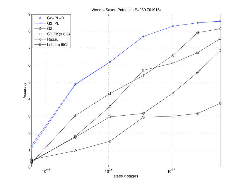
Figure 1: Resonance Problem using E=989.701916

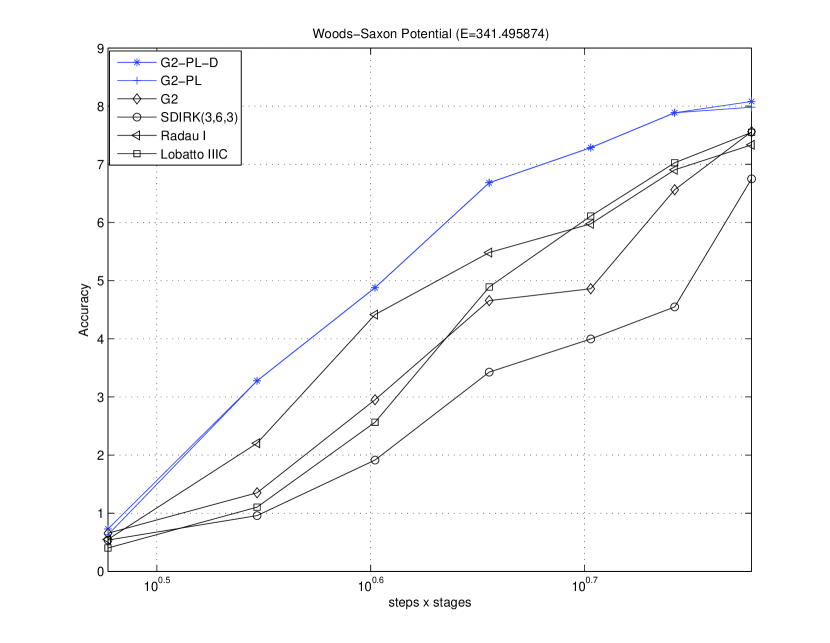
Figure 2: Resonance Problem using E=341.495874

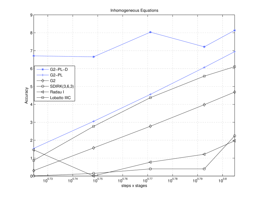
Figure 3: Inhomogeneous Equation

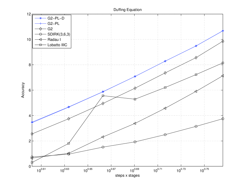
Figure 4: Duffing Equation

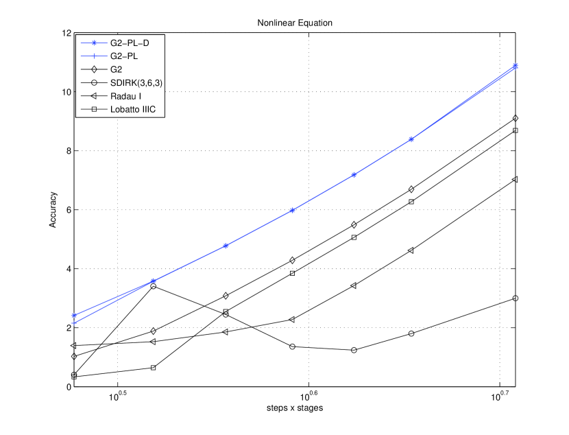
Figure 5: Nonlinear Problem

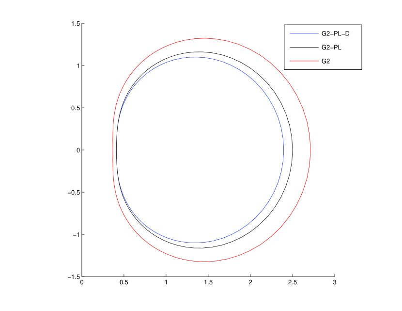
Figure 6: Stability region for the three implicit Runge-Kutta methods

References

- [1] D. Raptis and A.C. Allison, Exponential-fitting methods for the numerical solution of the Schrödinger equation, Computer Physics Communications, 14, 1 (1978)
- [2] L.Gr. Ixaru, M. Rizea, A Numerov-like scheme for the numerical solution of the Schrödinger equation in the deep continuum spectrum of energies, Comp. Phys. Comm. 19, 23-27 (1980)
- [3] A.D. Raptis, Exponentially-fitted solutions of the eigenvalue Schrödinger equation with automatic error control, Computer Physics Communications, 28, 427 (1983)
- [4] L. Gr. Ixaru and M. Rizea, Comparison of some four-step methods for the numerical solution of the Schrödinger equation, Computer Physics Communications, 38 (3) 329-337 (1985)
- [5] P. J. Van der Houwen and B. P. Sommeijer, Phase-Lag of Implicit Runge-Kutta methods, Society for Industrial and Applied Mathematics 26(1) 214-229(1989)
- [6] Toshiyuki Koto, Phase-Lag Analysis of Diagonally Implicit Runge-Kutta Methods, Journal of Information Processing 13(3), 361-366 (1990)
- [7] J. D. Lambert, Numerical methods for ordinary differential systems: the initial value problem, John Wiley & Sons, Inc., New York, NY (1991)
- [8] E. J. Haug, D. Negrut, C. Engstler, Implicit Runge-Kutta Integration of the Equation of Multibody Dynamics in Descriptor Form, Advances in Design Automation-Proceedings of the ASME Design Autmation Conference, Sacramento, CA (1997)
- [9] T.E. Simos, Four-step P-stable method with minimal phase-lag, Computer Physics Communications, 115, 1 (1998)
- [10] P. J. Van der Houwen, B. P. Sommeijer, Diagonally Implicit Runge-Kutta methods for 3D Shallow water applications, Advances in Computational Mathematics 12, 229 - 250 (2000)
- [11] T.E. Simos, P.S. Williams, A P-stable hybrid exponentially-fitted method for the numerical integration of the Schrödinger equation, Computer Physics Communications 131 (2000) 109-119
- [12] T.E. Simos An accurate eighth order exponentially-fitted method for the efficient solution of the Schrödinger equation, Computer Physics Communications 125 (2000) 21-59
- [13] T.E. Simos, Jesus Vigo-Aguiar, An exponentially-fitted high order method for long-term integration of periodic initial-value problems, Computer Physics Communications 140 (2001) 358-365
- [14] T.E. Simos, Jesus Vigo-Aguiar, A dissipative exponentially-fitted method for the numerical solution of the Schrödinger equation and related problems, Computer Physics Communications 152, 274-294 (2003)
- [15] J.C.Butcher, Numerical Methods for Ordinary Differential Equations, John Wiley & Sons, Ltd, Chichester, England (2003)
- [16] E. Hairer, G. Wanner, Solving Ordinary Differential Equations II. Stiff and Differential-Algebraic Problems, Berlin Heidelberg New York: Springer-Verlag (1996)
- [17] Z.A. Anastassi and T.E. Simos, Special optimized Runge-Kutta methods for IVPs with oscillating solutions, International Journal of Modern Physics C 15 1-15 (2004)
- [18] Z.A. Anastassi and T.E. Simos: A Dispersive-Fitted and Dissipative-Fitted Explicit Runge-Kutta method for the Numerical Solution of Orbital Problems, New Astronomy, 10, 31-37 (2004)
- [19] Z.A. Anastassi and T.E. Simos: A Trigonometrically-Fitted Runge-Kutta Method for the Numerical Solution of Orbital Problems, New Astronomy, 10, 301-309 (2005)
- [20] Z.A. Anastassi. and T.E. Simos, Trigonometrically Fitted Fifth Order Runge-Kutta Methods for the Numerical Solution of the Schrödinger Equation, Mathematical and Computer Modelling, 42 (7-8), 877-886 (2005)
- [21] Z.A. Anastassi and T.E. Simos, Trigonometrically-Fitted Runge-Kutta Methods for the Numerical Solution of the Schrödinger Equation, Journal of Mathematical Chemistry 3, 281-293 (2005)
- [22] Z.A. Anastassi and T.E. Simos, An optimized Runge-Kutta method for the solution of orbital problems, Journal of Computational and Applied Mathematics, 175, 1 (2005)
- [23] Z.A. Anastassi. and T.E. Simos, A Family of Exponentially-Fitted Runge-Kutta Methods with Exponential Order up to Three for the Numerical Solution of the Schrödinger Equation, Journal of Mathematical Chemistry, 41, 1, 79-100 (2007)
- [24] T.E. Simos, High-order closed Newton-Cotes trigonometrically fitted formulae for long-time integration of orbital problems, Computer Physics Communications 178, (2008), 199-207
- [25] J. M. Franco, I. Gomez, L. Randez, SDIRK methods for stiff ODEs with oscillating solutions, Applied Mathematics, 81, 197-209, (1997)